Modelling Development of Riparian Ranchlands Using Ecosystem Services at the Aravaipa Watershed, SE Arizona - MDPI
←
→
Page content transcription
If your browser does not render page correctly, please read the page content below
land
Article
Modelling Development of Riparian Ranchlands
Using Ecosystem Services at the Aravaipa Watershed,
SE Arizona
Laura M. Norman 1, * , Miguel L. Villarreal 2 , Rewati Niraula 3 , Mark Haberstich 4 and
Natalie R. Wilson 1
 1   U.S. Geological Survey, Western Geographic Science Center, 520 N. Park Avenue, Ste. #102K, Tucson,
     AZ 85719, USA; nrwilson@usgs.gov
 2   U.S. Geological Survey, Western Geographic Science Center, Menlo Park, CA 94025, USA;
     mvillarreal@usgs.gov
 3   Texas Institute of Applied Environmental Research (TIAER), Tarleton State University, Stephenville,
     TX 76402, USA; rewatin@gmail.com
 4   The Nature Conservancy, Aravaipa Canyon Preserve, Willcox, AZ 85643, USA; mhaberstich@tnc.org
 *   Correspondence: lnorman@usgs.gov; Tel.: 011-1-520-670-5510

 Received: 26 March 2019; Accepted: 14 April 2019; Published: 16 April 2019

 Abstract: This paper describes how subdivision and development of rangelands within a remote and
 celebrated semi-arid watershed near the US–Mexico border might affect multiple ecohydrological
 services provided, such as recharge of the aquifer, water and sediment yield, water quality, flow rates
 and downstream cultural and natural resources. Specifically, we apply an uncalibrated watershed
 model and land-change forecasting scenario to consider the potential effects of converting rangelands
 to housing developments and document potential changes in hydrological ecosystem services. A new
 method to incorporate weather data in watershed modelling is introduced. Results of introducing
 residential development in this fragile arid environment portray changes in the water budget,
 including increases in surface-water runoff, water yield, and total sediment loading. Our findings
 also predict slight reductions in lateral soil water, a component of the water budget that is increasingly
 becoming recognized as critical to maintaining water availability in arid regions. We discuss how the
 proposed development on shrub/scrub rangelands could threaten to sever imperative ecohydrological
 interactions and impact multiple ecosystem services. This research highlights rangeland management
 issues important for the protection of open space, economic valuation of rangeland ecosystem services,
 conservation easements, and incentives to develop markets for these.

 Keywords: hydrology; watershed modelling; water resources; scenario planning; sustainable
 management; ecosystem services

1. Introduction
     Ranchlands in the western United States are often used to raise livestock and grow various crops.
They are typically composed of a combination of privately-owned land and regulated grazing leases
on adjacent Federal or State allotments. In recent decades, rapid population growth and associated
cultural paradigms have incurred land-use change [1], including remote and arid rural landscapes
in the United States and Mexico borderlands [2,3]. Large historical cattle ranches get subdivided
into exurban landscapes and housing developments, or ranchettes, which fragment rangelands with
construction of roads and buildings [4]. Subdivision and development of large ranches can have
a variety of impacts on rangeland ecosystems, including the potential for increased nonnative plant and

Land 2019, 8, 64; doi:10.3390/land8040064                                           www.mdpi.com/journal/land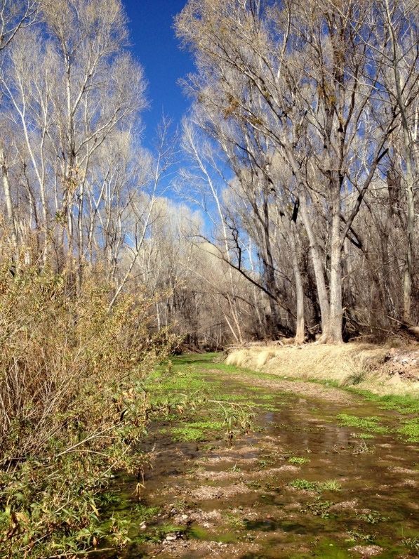
Land 2019, 8, 64                                                                                        2 of 21

animal species [5,6], soil disturbance, changes in prescribed fire or managed wildfire, and fragmented
wildlife habitat and travel corridors [7].
      Development of rangelands is also known to affect the function and character of local hydrology
in terms of changes to (i) peak flow, (ii) total runoff, (iii) quality of water, and (iv) hydrologic amenities,
defined as the appearance of a river [8]. Ellingson [9] proposed three watershed management
approaches for protecting the base flow of a river: (i) Artificial recharge to the aquifer; (ii) low-flow
augmentation using runoff impoundments; and (iii) restricting development. He suggested studies
to test the feasibility of these activities could be best conducted using calibrated rainfall-runoff or
groundwater flow models. In arid and semi-arid rangelands, biological diversity is closely linked
to the availability of water, and reducing the effects of land development on stream ecosystems is
a conservation priority. In the southwestern US, conservationists, ranchers, and forest workers are
trying to promote both environmental and economic sustainability on rangelands [10,11]. A mutual
goal is to balance production and conservation on interconnected landscapes and maintain cultural
and biological diversity for future generations.
      Historically, there has been a lot of research to understand the repercussions of varied land-use
within watersheds. Leopold [8] presented an application that forecasts conditions expected with
urbanization, which would explore scenarios based on different management options. Hydrology
and sedimentation models, coupled with urban growth or restoration scenarios, can be applied to
compare long-term water availability and tradeoffs in management practices [12–16]. Villarreal et al. [3]
developed future land-use scenarios in the binational Santa Cruz watershed, located on the border of
Arizona, United States, and Sonora, Mexico, to examine how biodiversity patterns are impacted by
land use change. The scenarios identified possible unintended consequences that may result from the
future implementation of regional conservation plans and portrayed some tradeoffs. For example,
Perkl et al. [17] coupled urban growth simulations with models of wildlife corridors to examine how
species migration might be adversely affected by development, and found that projected growth could
be mitigated to have less harmful impacts.
      Rangeland and riparian areas in the southwest were heavily impacted by livestock grazing in the
19th and early 20th centuries [18,19]. Overgrazing affected a wide range of ecosystem services, and
the debate over the relative ecological footprint of grazing vs. development (i.e., “cattle vs condos”)
continues to this day [6,20,21]. On one hand, because livestock are mobile, their footprint can be
large and affect a wide range of ecosystems (both upland and riparian) and ecosystem services [19].
Livestock trample and compact soils, causing erosion in both the uplands and riparian areas, with
impacts often lasting years after grazing pressure has subsided [22]. While the footprint of exurban
development may be more discrete, building may cause more direct habitat loss and fragmentation for
wildlife [23]. Bestelmeyer and Briske [24] suggest assessing and managing tradeoffs among ecosystem
services to guide adaptation and transformation in rangelands.
      Hydrologic ecosystem services describe the way ecosystems affect water resources, where
ecohydrological impacts on water quantity, quality, location, and timing, are portrayed in terms of
availability for humans [25–27]. Rangelands provide a suite of ecosystem services, including forage
for livestock production, habitat for wildlife, biodiversity, open space, carbon sequestration, fresh
water supply, and cultural services [10]. Norman et al. [14] outlined an approach to visualize declining
surface-water flows in unincorporated communities located within a 150-mile swathe of the border
between the US and Mexico. Socially and environmentally vulnerable communities may be more
receptive to incentive-based policy tools than more affluent communities.
      Food production from a rangeland-based industry is in decline, pressured by poor economic
returns, increased regulations, an aging rural population, and increasingly diverse interests of land
owners [10]. However, there are numerous other goods and services provided by rangelands that
can supply societal demands, such as clean water, pollinator services, and food supplies. Payment
for Ecosystem Services (PES) programs can compensate or subsidize landowners for producing or
maintaining environmental services [28]. With proper incentives and economic benefits, rangelands
Land 2019, 8, 64                                                                                    3 of 21

can provide both historical and more unique goods and services [10]. PES may be particularly suited
to rural ranching communities and ranchettes in the US–Mexico borderlands [29].
      The Aravaipa Watershed in southeastern Arizona, USA, contains Federally-protected perennial
creek flows and wilderness areas, and culturally important rangelands, approximately 135 km north
of the US–Mexico border. Some Aravaipa Valley ranches have recently (between 2004–2008) split
off privately-owned parcels. According to the Aravaipa Watershed Conservation Alliance (AWCA;
personal communication), approximately 300 ~16 ha lots are currently being considered for conversion
to ranchettes, with associated roads, plumbing, well-excavation, and electrical expansion imminent.
Additionally, county taxes are delinquent on some of these lots and many are currently re-listed for sale
at this time. While these ranches were subdivided and sold during the real-estate boom, it is the local
contention that the properties have subsequently lost value. The goal of this research is to help qualify
and document the value, aside from realty dollars, associated with hydrologic ecosystem services lost
or gained from varying land-management strategies, that might be vetted for PES incentives.

2. Methods
     We describe our study area, followed by the two main components of research. First, we applied
a daily time step hydrological model to simulate 36 years of rainfall and runoff, and developed estimates
of watershed response spatially, to examine the water budget. Second, we modified the land cover
input of the model to simulate how low-density development of ranchettes on some private lands
might affect the expected hydrological response within the watershed and how ecosystem services
may respond to these changes.

2.1. Study Area
     Aravaipa Canyon lies astride Graham and Pinal Counties, Arizona, USA, just south of and
adjacent to the San Carlos Apache Reservation (Figure 1). The ~140,000 ha watershed is removed from
urban centers and access is limited by topography and lack of roads. Increasing livestock and mining
developments began in the 1890s and by the 1920s, mining thrived, goat and human populations
surged, and livestock roamed the open range [30].
     In 1980, the advocacy group Defenders of Wildlife expressed concern about the effects of increased
water demand in Aravaipa [9]. Renowned ichthyologist Wendell Minckley [31] suggested that monthly
flows varied between 0.28–0.71 cubic meters per second (cms) while maintaining an average of 0.42 cms,
and the US Bureau of Land Management (BLM) applied to the Arizona Department of Water Resources
(ADWR) for a permit to appropriate this average to sustain fish, wildlife, and recreation [32]. Adar and
Neuman [33] suggested that to preserve the habitat of the canyon, the recharge area at the east entrance
to the Canyon must be conserved.
     In 1984, Congress designated ~2711 ha of the lower Canyon and surrounding area a “wilderness
area” (P.L. 98-406,98 Stat. 1485) and then expanded this to ~8094 ha in the Arizona Desert Wilderness Act
of 1990 (H.R.2570 - 101st Congress (1989–1990)). The BLM manages the Aravaipa Canyon Wilderness
while allowing for limited primitive and unconfined recreation (Figure 1). In 1989, the third instream
flow permit (Number 33-87114) in Arizona’s history was issued at Aravaipa, effectively protecting
the average monthly flow of 0.42 cms required (~0.28 cms for fish and wildlife and ~0.14 cms for
recreation) from appropriation by subsequent junior surface water claimants. This protected natural
conditions and flow of Aravaipa Creek based on Federal and State water rights [34].
     Currently, privately-owned land within the watershed (~21,793 ha) includes 18 ranches that also
hold Federal and/or State allotments and leases for livestock grazing (Figure 1). Among the public
lands present, only Aravaipa Canyon itself is not grazed as an allotment [32]. Management of the
leased acreage is divided by the following agencies: State Trust ~53,343 ha, US Forest Service ~34,383 ha,
BLM ~28,021 ha, The Nature Conservancy (TNC) ~3642 ha, and some smaller parcels managed by the
San Carlos Apache Tribe and other Indian tribes, with allotments ~1755 ha (Figure 1). The amount of
forage authorized on BLM allotments in the Aravaipa area is 9306 Animal Unit Months (AUMs) [32].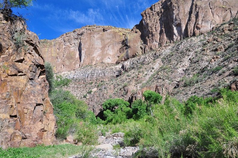
Land 2019, 8, 64                                                                                             4 of 21

In general, most of these ranches have reduced numbers of cattle compared to 20 years ago, due to
long2019,
Land term 8, drought  and
             x FOR PEER   reduced carrying capacity.
                        REVIEW                                                              5 of 22

      Figure 1.
              1. Location
                  Locationof of
                              thethe
                                   Aravaipa Watershed
                                     Aravaipa WatershedBasin  (red(red
                                                          Basin     outline) within
                                                                       outline)     the the
                                                                                within  StateState
                                                                                               of Arizona, the
                                                                                                   of Arizona,
      landownership,   major  streams, USGS  gaging station, and  Wilderness  boundary.
      the landownership, major streams, USGS gaging station, and Wilderness boundary.

2.1.1.Conservation
       Environmentalincentives
                       Setting authorized by the 2002 Farm Bill include donated and purchased
conservation easements by national non-governmental organizations such as TNC [10]. TNC prioritizes
      The climate is semi-arid; annual precipitation ranges from 36 to 71 cm. Aravaipa Creek, a
tributary of the San Pedro River, runs south to north, through Klondyke and then west, where it
enters Aravaipa Canyon (Figure 1). It is mostly ephemeral (has flowing water for brief periods in
response to rainfall), but is normally dry from the headwater to the intersection with Stowe Gulch
[9]. From this intersection to the west, where there is a USGS stream gage station (#09473000 Aravaipa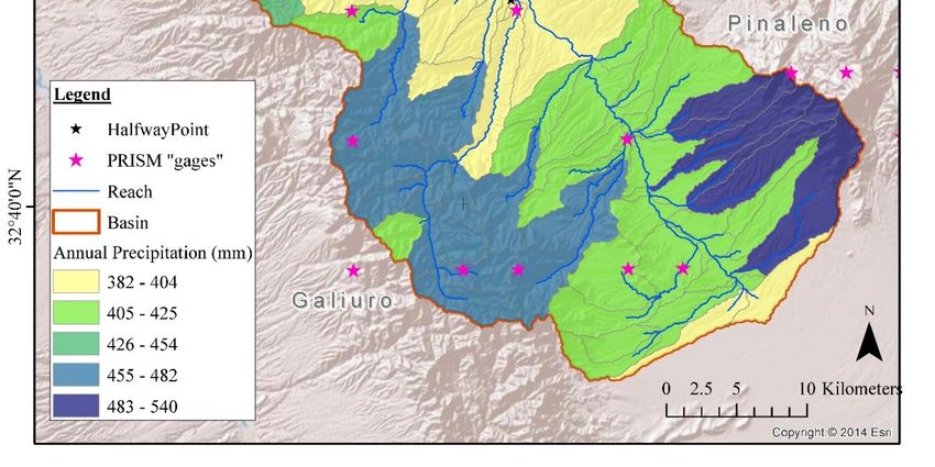
Land 2019, 8, 64 5 of 21
balancing the needs of people and nature to ensure that conservation is a critical outcome in economic
development. Conservation-easement agreements usually hinder development and support on-going
stewardship of natural resources by ranchers and other private landowners [10]. TNC maintains a goal
to ensure the long-term protection of the Aravaipa Creek stream system.
In 1991, Hadley et al. [30] noted that due to abundant water with little usage in Aravaipa,
a watershed conservation organization was unnecessary, but given a need to coordinate upstream
and downstream practices and erosion control, it might be desirable. In response to the shared goal
to preserve and sustain Aravaipa Valley’s natural landscapes by means of watershed and rangeland
restoration, the Aravaipa Watershed Conservation Alliance (AWCA) formed in 2016, joining nonprofit
groups, private landowners and agency staff. In 2017, AWCA engaged the USGS to consider how
watershed models could be used to simulate surface-water runoff and recharge under various land-use
conditions to demonstrate how people can affect the future of their water resources [35]. AWCA is
interested in understanding how low-density residential development on privately owned portions of
ranches in the upper watershed could affect ecosystems and water supplies.
2.1.1. Environmental
Land 2019, Setting
8, x FOR PEER REVIEW 6 of 22
The climate is semi-arid; annual precipitation ranges from 36 to 71 cm. Aravaipa Creek, a tributary
Creek near Mammoth; Figures 1 and 2), Aravaipa Creek is perennial, but again becomes ephemeral
of the San Pedro
downstream River, runs south to north, through Klondyke and then west, where it enters Aravaipa
of that.
Canyon (Figure 1). It is mostly
The gaging station has beenephemeral (has since
in operation flowing water
1987, for brief
operated periods
through theincooperation
response toofrainfall),
Pinal
but is normally dry from the headwater to the intersection with Stowe Gulch [9].
County and the USGS AZ Water Science Center Tucson Field Office. At the gage, discharge From this intersection
to the west, where
measurements there is
average a USGS
~0.62 cms.stream gage[9]station
Ellingson (#09473000
suggests Aravaipa
the runoff ratio isCreek
~3.3%near
withMammoth;
springs
Figures 1 and 2), Aravaipa Creek is perennial,
sustaining the creek during drier periods. but again becomes ephemeral downstream of that.
140 0
120 2
Cubic Meters per Second (CMS)
100 4
6
Precipitation (cm)
80
8
60
10
40
12
20
14
0
1988
1989
1990
1991
1992
1993
1994
1995
1996
1997
1998
1999
2000
2001
2002
2003
2004
2005
2006
2007
2008
2009
2010
2011
2012
2013
2014
2015
2016
2017
2018
Precip. (cm.) CMS
Figure 2.2. Rainfall-runoff
Figure Rainfall-runoff response
response portrayed
portrayed in
in hyeto-hydrograph
hyeto-hydrographatat USGS
USGSstream
streamgage
gagestation
station
#09473000,Aravaipa
#09473000, Aravaipa Creek
Creek near
near Mammoth
Mammoth Springs.
Groundwater
The moveshas
gaging station from recharge
been areas in since
in operation the high-elevation
1987, operatedmountain
throughblocks and along theof
the cooperation
mountain fronts towards Aravaipa Creek on the central valley floor (Figure
Pinal County and the USGS AZ Water Science Center Tucson Field Office. At the gage, 3a), and hence
discharge
downgradient average
measurements to the discharge
~0.62 cms.area near the
Ellingson confluence
[9] suggests thewith
runoffStowe Gulch
ratio is ~3.3%[9,36,37]. The
with springs
underground
sustaining water during
the creek moves drier
up toperiods.
396 m/day [9,30]. Groundwater recharge and discharge at springs
is likely dependent on precipitation [32]. Ellingson [9] estimated ~2.4% (14.3 MIL m3) of the
watershed's annual precipitation reaches the groundwater reservoirs. Other groundwater recharge
estimates from infiltrating precipitation and runoff range from 8.6 MIL m3 to 20.6 MIL m3 [38]. Adar
and Neuman [33] applied a model that shows lateral recharge from the pediments and the tributary
Stowe Gulch Basin to be the main source of replenishment to the water table aquifer (~77 mm of deep
percolation per year over approximately 111 km2 of the basin). Lateral flows are critically important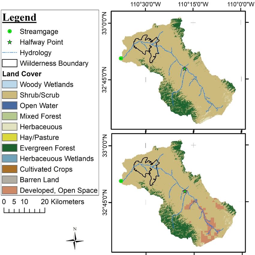
Land 2019, 8, 64 6 of 21
Groundwater moves from recharge areas in the high-elevation mountain blocks and along
the mountain fronts towards Aravaipa Creek on the central valley floor (Figure 3a), and hence
downgradient to the discharge area near the confluence with Stowe Gulch [9,36,37]. The underground
water moves up to 396 m/day [9,30]. Groundwater recharge and discharge at springs is likely
dependent on precipitation [32]. Ellingson [9] estimated ~2.4% (14.3 MIL m3 ) of the watershed’s
Land 2019, 8, x FOR PEER REVIEW 7 of 22
annual precipitation reaches the groundwater reservoirs. Other groundwater recharge estimates from
infiltrating precipitation and [9].
runoff range 3 to 20.6 MIL m3 [38]. Adar and Neuman [33]
River on younger alluvium Along thefrom 8.6 axis
central MILof mthe valley, the young alluvium is separated
applied
from olda model
alluviumthatby
shows lateral recharge
low permeability from
layers. the the
Here pediments and the tributary
young alluvium provides Stowe Gulch
a shallow Basin
water
totable
be the main source of replenishment to the water table aquifer (~77 mm of deep percolation
unconfined aquifer and the old alluvium forms a confined aquifer [36,41]. The older alluvium per year
over approximately 111 km 2 of the basin). Lateral flows are critically important in dry seasons, with
abruptly ends near the top of the canyon, where a fault has displaced the Hellhole Conglomerate
some
down upward
againstleakage from the
the relatively underlyingvolcanic
impermeable confined aquifer
rocks. This[33].
structure forces water in the c
(a) (b)
(c) (d)
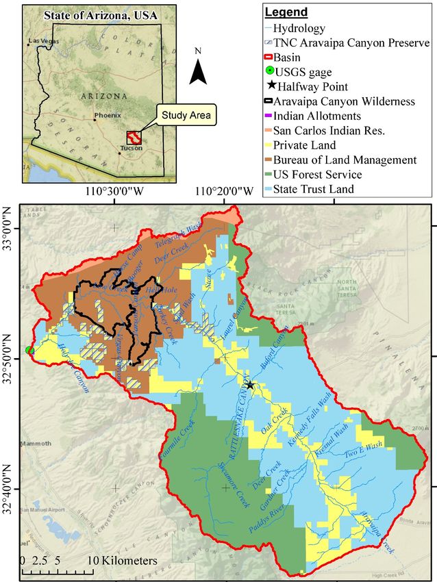
Figure3.3.Photographs
Figure Photographs of
of (a) upper watershed,
watershed,(b)
(b)narrow
narrowand
anddeep
deepbasin,
basin,(c)(c)
“Aravaipa Spring”
“Aravaipa and
Spring” and
(d)mainstem
(d) mainstemofofcreek.
creek.
2.1.2. Ecosystem Services
The Millennium Ecosystem Assessment [42] was the first to systematically define ecosystem
services. Even before this assessment, Hadley et al. [30] described some goods and services in the
Aravaipa Canyon being provided by nature. Goods included food, crops, fuelwood, fish, game, furs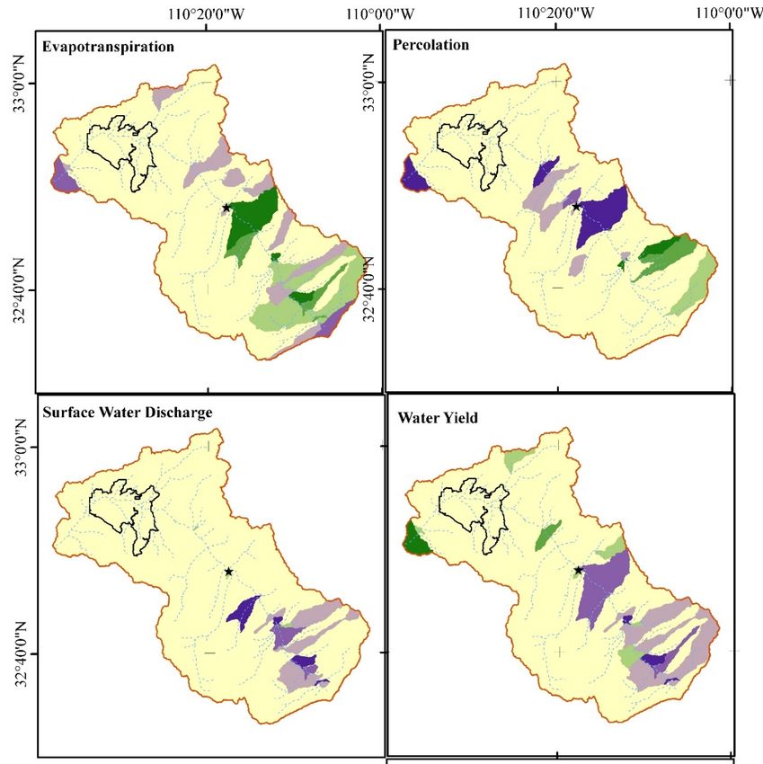
Land 2019, 8, 64                                                                                       7 of 21

     Small rural communities exist in the riparian corridor at both ends of the watershed and use the
instream flow for irrigation, stock watering, and household use [39]. The narrow and deep Aravaipa
basin (Figure 3b) was formed by displacement of the valley downward, relative to the mountains on
each side, along normal faults forming the graben structure seen today [9,33]. Three of the Arizona
“Sky Islands” mountain ranges border Aravaipa basin: (i) Santa Teresa (north-eastern), (ii) Pinaleno
(southeastern), and (iii) Galiuro (southwestern).
     Along the upper mainstem of Aravaipa Creek, the river is situated in mostly sedimentary deposits,
consisting of loosely- to firmly-consolidated gravel, sand and silt, local clay, gypsum, marl, limestone,
diatomite, and some intercalated basalt flows and felsic tuff beds [40]. The location of “Aravaipa
Spring” and the beginning of perennial flow is controlled by the presence of bedrock (Figure 3c).
Aravaipa Creek flows from its headwaters northwest to its confluence with the San Pedro River on
younger alluvium [9]. Along the central axis of the valley, the young alluvium is separated from
old alluvium by low permeability layers. Here the young alluvium provides a shallow water table
unconfined aquifer and the old alluvium forms a confined aquifer [36,41]. The older alluvium abruptly
ends near the top of the canyon, where a fault has displaced the Hellhole Conglomerate down against
the relatively impermeable volcanic rocks. This structure forces water in the confined aquifer upward,
and is responsible for the perennial flow found in Aravaipa Creek [9] (Figure 3d).

2.1.2. Ecosystem Services
       The Millennium Ecosystem Assessment [42] was the first to systematically define ecosystem
services. Even before this assessment, Hadley et al. [30] described some goods and services in the
Aravaipa Canyon being provided by nature. Goods included food, crops, fuelwood, fish, game,
furs and minerals and services such as diluting and cleansing polluted air and water, filtering and
chemically transforming harmful mining residuals, manufacturing and supplying plant nutrients (from
photosynthesis and soil supplies), and conditioning microclimates. While some of these more tangible
resources have obvious economic and social value, some are yet to be quantified. The Millennium
Ecosystem Assessment [42] grouped ecosystem services into four categories: (i) provisioning;
(ii) regulating; (iii) supporting; and (iv) cultural.
       Provisioning ecosystem services are the products that humans obtain from ecosystems including
water, food, and habitat for wildlife. “Any desert canyon with permanent water, like Aravaipa, will be
as full of life as it is beautiful” [43]. The abundance of water (rain and soil moisture) determines the
abundance of crops and rangeland. A critical provisioning service to rangelands includes management
practices that maintain ecological functions or restore functions to systems that have been degraded [10].
       Regulating ecosystem services maintain the quality of air and soil, provide flood control, or pollinate
crops. Flooding, like erosion, can be important for ecosystems but regulation is important [44]. While
air and water quality enhancement have clear implications for human use, they also contribute to
the quality of habitation of critical fish and wildlife species. Ecosystem services in the Canyon that
benefit wilderness and wildlife are barely understood and largely unquantified [39]. The effects of land
clearing and cultivation, livestock, mining and road building on soils have not been well documented in
Aravaipa [30], yet the current inhabitants express great interest in protection of the environment.
       Supporting ecosystem services are those that provide living spaces for plants and animals
as well as maintain their diversity. Along the riparian zone, where water is available to support them,
cottonwood, Arizona walnut, alder, willow, mesquite, box elder, and other vegetation grow to provide
habitat for more than 200 species of birds, 46 species of mammals, 46 reptilian species, and 8 amphibian
species that reside in the wilderness area [34], and the Aravaipa watershed and riparian corridor have
been identified as important breeding habitat for the Federally threatened yellow-billed cuckoo [45].
Depth to water table sets the upper limit of a riparian species’ elevation, while ability to tolerate
scour may set the lower limit [32]. In 1966, seven native fish species were documented at Aravaipa,
the densest native population in the state [46]. The perennial nature of the water supply supports this
habitat. Fish habitat is controlled by patterns of erosion, sediment transport, and deposition, which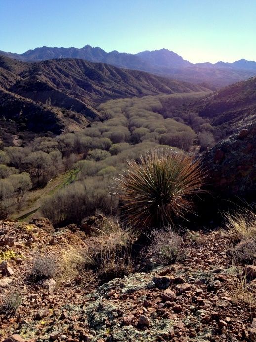
Land 2019, 8, 64                                                                                   8 of 21

in turn are functions of precipitation, runoff, and bed load volume [46]. Flood magnitudes vary over
a period of hours along with corresponding changes in turbidity, while water temperatures can change
from ~16–40 ◦ C annually [46,47].
     Cultural services are nonmaterial benefits or experiences that people obtain from ecosystems.
Aravaipa has great value as an aesthetic resource and beauty is abundant [30]. A variety of outdoor
recreationists use the ecosystem for hiking, hunting, picnicking, birding, horseback riding, primitive
camping, off-highway vehicle driving, geocaching, and playing in the stream [32]. In fact, the canyon
is such a popular destination for outdoor enthusiasts, that the BLM turned to a permit system to limit
the number of visitors and reduce human impacts to the area. Moore et al. [34] found that water
was rated by visitors as the most important attribute in the recreational setting of Aravaipa Canyon.
Weber and Berrens [39] discussed that the instream flow allocation for recreation represents significant
worth to society. And the rural or ranching cultural history values are plentiful. At Aravaipa Canyon,
the relatively small floodplain discouraged large human settlements that grew up along other Arizona
perennial rivers and the rugged terrain provided sanctuaries for wildlife and reduced extinction
rates [30]. The enormous biodiversity provides services that have yet to be fully characterized, such as
species that provide habitat for pollinators or species with medicinal value. Effects that the loss or
degradation to environmental factors, such as in soil nutrient wealth and depth to bedrock or water,
would have on biodiversity are unknown.

2.2. Hydrological Model Application
      The Soil and Water Assessment Tool (SWAT) is a semi-distributed model, jointly developed by
USDA Agricultural Research Service (USDA-ARS) and Texas A&M AgriLife Research, a part of the
Texas A&M University System [48]. It is a long-term yield model, that uses daily average values as input.
SWAT has been applied to predict the effect of land use, management practices, and climate change on
water, sediment, and agricultural chemical yields in small- to large-scale watersheds with varying soils,
land use, and management over extended periods of time [48,49]. It is oft used in assessing erosion
control, non-point source pollution control, and best management in watersheds [13,14,16,50–54].
      In watershed-modeling studies, flow is often calibrated at the watershed outlet. However,
in arid and semi-arid watersheds, flow characteristics vary throughout the watershed and is often
discontinuous for most of the year, except during large flood events. In a SWAT calibration at the
nearby Santa Cruz River Watershed, calibration was performed at 7 monitoring stations throughout
the watershed to improve model reliability [53]. Results portray that each station required different
variations of controlled parameters to match flow predictions in the model at that site. However, when
the model was calibrated at only the watershed outlet, flow predictions at the other monitoring stations
proved inaccurate. Uncalibrated watershed models have been used in a number of applications for
assessing relative change [55,56]. Uncalibrated physically based models can also be used with some
confidence in identifying the trends and directions of changes in watershed response due to changes in
watershed conditions and are a valuable aid in identifying where conservation efforts might be focused
to offset impacts from LULC [53,56,57]. In this study, we use the uncalibrated model for assessing the
relative change in hydrology and associated ecosystem services resulting from conversion of rangeland
to housing development.

SWAT Model Development and Parametrization
     We obtained soils, topography and land-use data from various sources and organized them in
a geodatabase. Soils were mapped by the USDA Natural Resources Conservation Service (NRCS) at
a scale of 1:12,000, in the Soil Survey Geographic Database (SSURGO) data [58]. The USGS National
Land Cover Database is a 16-class land-cover classification based on the Landsat Enhanced Thematic
Mapper+ (ETM+) from 2011 at a spatial resolution of 30 m [59]. A 10 m digital elevation model (DEM)
was input into SWAT to delineate watershed boundaries, where stream channels were constricted
to represent ~722 ha. The USGS gage was identified as the outlet to drain to, creating a total area of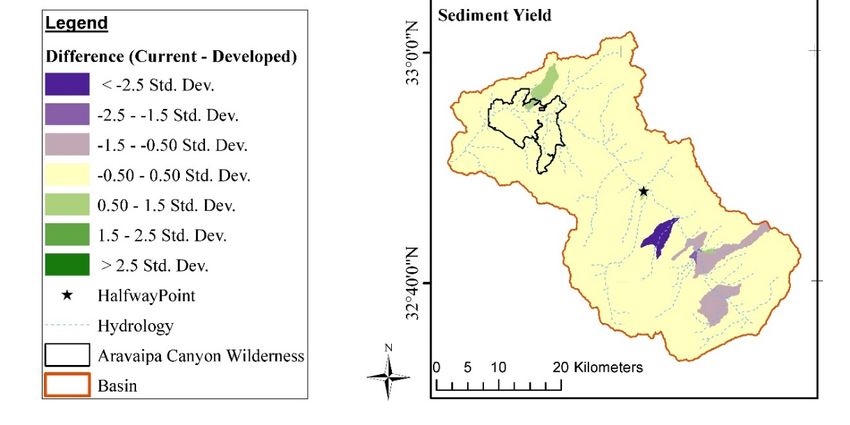
Land 2019, 8, 64                                                                                  9 of 21

139,296 ha to be modeled. All geospatial data were trimmed to represent the study area and converted
to a common Universal Transverse Mercator (UTM) projection.
       SWAT model requires continuous slope values to be discretized into multiple classes (3) with
limits 0%–10%, 10%–30%, and >30%. The watershed was subdivided into 734 discreet hydrologic
response units (HRUs), within 117 sub-basins. We defined the weights of the HRU thresholds equally
to represent 10% over sub-basin, land use, and soil areas. The model was run for 36 years, starting in
1981, with daily rainfall derived runoff estimated using the curve number method.
       At first, we used an observed/measured rainfall dataset of 2 gages for the watershed to drive the
rainfall in the model but found our biased data capture skewed the precipitation distribution. There is
always uncertainty attributed to the precipitation input, and even when a watershed is heavily gaged,
it is hard to document all the storms that might occur and not over-extrapolate. We simulated weather
using the weather generator in SWAT with multiple gages simulated for the watershed and it created
inaccurate estimates of higher precipitation in the western side of the watershed, which tapered to the
east. The SWAT weather generator portrayed the same bias as the real rain gage dataset, which was
ultimately driven by the weather generator. It was unable to capture the high-elevation precipitation
we knew to be occurring in the Pinaleño and Galiuro Mountain ranges, but instead depicted high
rainfall towards the outlet. This is very different from what land managers see on the ground, where
the upper watershed in the southwest is grassland and oak savanna, indicating more precipitation,
while the area to the northwest, where the USGS gage is located, is in saguaro cacti and creosote
shrublands, a drier regime.
       In order to resolve the error in spatially distributed precipitation as extrapolated by the SWAT
model from station (point) data, we downloaded 35 years of daily weather raster data (precipitation)
available at a 4 km spatial scale from PRISM (http://www.prism.oregonstate.edu). The PRISM Climate
Group [60] gathers climate observations from a wide range of monitoring networks, with quality-control
measures, and develops spatial climate datasets that portray short-term and long-term climate patterns.
We used the centroid of each PRISM grid cell to create a proxy “station” for use in SWAT. We selected
stations that best represent the spatial and climatic variability of this watershed, based on topography
and local knowledge. PRISM grid points were mostly supplemented for the areas where the observed
meteorological station was scarce and not representative of the actual precipitation due to spatial
heterogeneity of topography and rainfall along that northern part of the watershed. All SWAT model
input parameters are improved given actual physical knowledge of the watershed, which is true for
most physically-based models [61]. After some trial and error, 20 virtual “gages” scattered within the
watershed with additional gages around it appear to portray the elevation associated spatial patterns
evidenced in the climate normal pattern, with one gage per ~70 km2 of watershed area. The data were
formatted appropriately to use as weather data input (Figure 4).
actual physical knowledge of the watershed, which is true for most physically-based models [61].
After some trial and error, 20 virtual “gages” scattered within the watershed with additional gages
around it appear to portray the elevation associated spatial patterns evidenced in the climate normal
pattern, with one gage per ~70 km2 of watershed area. The data were formatted appropriately to use
Land
as 2019, 8, 64
weather data input (Figure 4). 10 of 21
Figure 4. Distribution of precipitation based on synthesized gage dataset to represent daily rainfall
Figure 4. Distribution
summarized of precipitation
to 2016 annual values. based on synthesized gage dataset to represent daily rainfall
summarized to 2016 annual values.
2.3. Scenario Assessment
2.3. Scenario Assessment
The use of watershed hydrologic models, designed specifically to simulate surface and near-surface
processes, canofaid
The use in visualizing
watershed potential
hydrologic effects
models, of landspecifically
designed management decisionssurface
to simulate on surface-water
and near-
hydrology
surface and the can
processes, groundwater system. Logsdon
aid in visualizing potentialand Chaubey
effects [44]management
of land developed mathematical
decisions onindices to
surface-
represent ecosystem service quantities using the outputs SWAT. We consider the provisional and regulatory
ecosystem services they describe: Fresh water provisioning, food provisioning, fuel provisioning, erosion
regulation and flood regulation, to compare ecosystem services within a watershed, given two different
land management scenarios.
In Aravaipa, some land owners are dividing ranches into ranchettes and developing the riparian
area to supplement incomes (Mark Haberstich personal observation 2018). In order to simulate this
land-change scenario, the National Land Cover Database (NLCD) data from 2011 was downloaded and
mapped for the watershed (Figure 5, top). To simulate conversion of ranchland to ranchettes, all pixels
falling within privately-owned parcels in the upper watershed were changed to “Developed” to reflect
potential land cover changes (Figure 5, bottom). Developed, Open Space areas were defined as a mix of
constructed materials, but mostly vegetation, where impervious surfaces account for less than 20% ofprovisioning, fuel provisioning, erosion regulation and flood regulation, to compare ecosystem
services within a watershed, given two different land management scenarios.
In Aravaipa, some land owners are dividing ranches into ranchettes and developing the riparian
area to supplement incomes (Mark Haberstich personal observation 2018). In order to simulate this
land-change scenario, the National Land Cover Database (NLCD) data from 2011 was downloaded
and mapped for the watershed (Figure 5, top). To simulate conversion of ranchland to ranchettes, all
Land 2019, 8, 64 11 of 21
pixels falling within privately-owned parcels in the upper watershed were changed to “Developed”
to reflect potential land cover changes (Figure 5, bottom). Developed, Open Space areas were defined
as a mix of constructed materials, but mostly vegetation, where impervious surfaces account for less
total land cover
than 20%[59]. The land
of total SWAT model
cover [59]. was then applied
The SWAT model wasto then
bothapplied
the baseline
to both and developed
the baseline and scenarios
and differences between
developed the
scenarios two
and were assessed.
differences between the two were assessed.
Figure 5. Current (top) and developed (bottom) land use inputs for SWAT (Soil and Water
Figure 5. Current (top) and developed (bottom) land use inputs for SWAT (Soil and Water Assessment
Assessment Tool) scenario assessment, modified from the NLCD [59].
Tool) scenario assessment, modified from the NLCD [59].
When interpreted by the SWAT model, this created an increase in low-density urban land use
and an almost equivalent decrease in Range-Brush along the riparian area (in privately owned lands),
affecting ~5600 ha (4% of the total watershed area).
3. Results
The analyses and maps include a halfway point in the Aravaipa Creek watershed, near the centroid
of the polygon (UTM: 12N 563257, 3627291; Figure 1). We designated this to look at the impacts directly
below where our changing land-use is set to occur. We compare it with the outlet of the entire watershed
(USGS Gaging Station) to discern how those immediate impacts are diffused over time and space. It is
noted that the model has not simulated a change in land use at a specific time frame but rather, examines
what the land use change would look like at any year of the iteration. Obviously, this did not occur in
the past, but is meant to portray the impacts of such a change into the future, based on the previous
climate record.
In examining the model results for both daily and monthly simulations for the 36-year simulation
(1981–2016), we present the ending yearly totals from 2016, a relatively normal year precipitation-wise,
to examine changes in discharge and concentration of sediment. Spatial variations on the landscape
are portrayed for percolation, surface water runoff, water yield, evapotranspiration and sediment yield.
The differences between the current land use and the proposed ranchette development are compared.
Additionally, the average annual results for both scenarios are discussed.the future, based on the previous climate record.
In examining the model results for both daily and monthly simulations for the 36-year
simulation (1981–2016), we present the ending yearly totals from 2016, a relatively normal year
precipitation-wise, to examine changes in discharge and concentration of sediment. Spatial variations
on the landscape are portrayed for percolation, surface water runoff, water yield, evapotranspiration
and8,sediment
Land 2019, 64 yield. The differences between the current land use and the proposed ranchette 12 of 21
development are compared. Additionally, the average annual results for both scenarios are
discussed.
3.1. Discharge
3.1. Discharge
Results show simulated increased surface discharge on the landscape in the main channel or reach
files. ThisResults show simulated
is represented increased
as increased surface
daily discharge
streamflow inon
thethe landscape
reaches in the mainwhere
downstream, channelsimulated
or
reach files. This is represented as increased daily streamflow in the reaches downstream, where
average annual flow is increased by ~0.04 cms at our halfway point and ~0.03 cms at the USGS gaging
simulated average annual flow is increased by ~0.04 cms at our halfway point and ~0.03 cms at the
station (Figure 6).
USGS gaging station (Figure 6).
Difference Hydrograph
USGS Gage (Dev - Current) Halfway Point (Dev - Current)
Cubic Meters per Second (cms)
0.08
0.07
0.06
0.05
0.04
0.03
0.02
0.01
0
Years
Figure
Figure 6. Difference
6. Difference in dischargebetween
in discharge between Current
Current and
andDeveloped
Developedscenarios, at Watershed
scenarios, Halfway
at Watershed Halfway
Point and USGS Gaging Station, from uncalibrated SWAT model iterations.
Point and USGS Gaging Station, from uncalibrated SWAT model iterations.
3.2. Sedimentation
3.2. Sedimentation
The simulated increased sediment yield extends into the river, represented as increased
The simulated increased sediment yield extends into the river, represented as increased concentration
concentration of sediment in the reach during the timestep, accessed in SWAT output files and
of sediment
Land 2019,in
8, xthe
FORreach during the timestep, accessed in SWAT output files and described
PEER REVIEW 13 of 22in the main
channel or reach files. Simulated sediment concentration average is increased by ~0.19 mg/kg (ppm) at
described in the main channel or reach files. Simulated sediment concentration average is increased
our halfway point but is negligible at the USGS gaging station (Figure 7).
by ~0.19 mg/kg (ppm) at our halfway point but is negligible at the USGS gaging station (Figure 7).
Difference in Sediments
USGS Gage (Dev - Current) Halfway Point (Dev - Current)
Sediment concentration (mg/kg)
1
0.8
0.6
0.4
0.2
0
-0.2
-0.4
1986
1987
1988
1989
1990
1991
1992
1993
1994
1995
1996
1997
1998
1999
2000
2001
2002
2003
2004
2005
2006
2007
2008
2009
2010
2011
2012
2013
2014
2015
2016
Years
Figure
Figure 7. Difference
7. Difference in sediment
in sediment concentration
concentration between
between Currentand
Current andDeveloped
Developedscenarios,
scenarios, at
at Watershed
Watershed Halfway Point and USGS Gaging Station, from uncalibrated SWAT model iterations.
Halfway Point and USGS Gaging Station, from uncalibrated SWAT model iterations.
3.3. Spatial Distribution
Most important to the individual land managers was the effect that development might have on
their ranches, portrayed by SWAT output variables describing sub-basins. Modeling shows most
change occurs in the upper watershed where the development occurred (Figure 8). Changes in
evapotranspiration show both increases and decreases. Percolation decreases in the upper watershed
and increases on the lower watershed, especially around Aravaipa Spring. Without knowledge of theLand 2019, 8, 64 13 of 21
3.3. Spatial Distribution
Most important to the individual land managers was the effect that development might have on their
ranches, portrayed by SWAT output variables describing sub-basins. Modeling shows most change occurs
in the upper watershed where the development occurred (Figure 8). Changes in evapotranspiration
show both increases and decreases. Percolation decreases in the upper watershed and increases on the
lower watershed, especially around Aravaipa Spring. Without knowledge of the groundwater aquifer
boundaries feeding into the spring discharge and well table connectivity, it is hard to say how this affects
water users. Surface-water discharge and water yield increases in the upper watershed based on the
scenario change.
Land Sediment
2019, 8, x FOR yield increased there as well as in downstream sub-watersheds.
PEER REVIEW 14 of 22
Figure 8. Difference in results between Current and Developed scenarios, from uncalibrated SWAT
Figure 8. Difference in results between Current and Developed scenarios, from uncalibrated SWAT
model iterations, where values above standard deviation (Std. Dev.; purple) show increased, and
model iterations, where values above standard deviation (Std. Dev.; purple) show increased, and
values values
belowbelow
Std. Dev. (Green) depict decreases.
Std. Dev. (Green) depict decreases.
3.4. Basin-wide Change
In comparing the output files from each simulation, there are some notable changes in average
annual basin stress values, including a small increase in surface-water runoff and yield, and totalLand 2019, 8, 64 14 of 21
3.4. Basin-wide Change
In comparing the output files from each simulation, there are some notable changes in average
annual basin stress values, including a small increase in surface-water runoff and yield, and total
sediment loading, along with a small decrease in lateral soil discharge and ET, based on the increased
development (Table 1). As expected, the changes look less significant at the basin scale when compared
at the sub-basin scale, where changes are more significant. There are also changes in average annual
basin nutrients, based on the increased development, especially noted are the increase in nitrogen and
decrease in phosphorus.
Table 1. Differences in average annual basin output values between Current and Developed scenarios.
Current Developed Difference Units % Change
PRECIP 425.4 425.4 0 MM 0
SURFACE RUNOFF DISCHARGE (Q) 18.13 18.99 0.86 MM 5
LATERAL SOIL Q 83.02 82.71 −0.31 MM 0
TOTAL WATER YIELD 104.09 104.71 0.62 MM 1
GROUNDWATER (SHALLOW
2.3 2.35 0.05 MM 2
AQUIFER) Q
DEEP AQUIFER RECHARGE 0.63 0.64 0.01 MM 2
PERCOLATION OUT OF SOIL 12.68 12.84 0.16 MM 1
TOTAL AQUIFER RECHARGE 12.7 12.86 0.16 MM 1
EVAPOTRANSPIRATION 311.3 310.6 −0.7 MM 0
TOTAL SEDIMENT LOADING 2.47 2.52 0.05 T/HA 2
4. Discussion
We used an uncalibrated SWAT model for assessing relative change in hydrology and associated
ecosystem services resulting from conversion of rangeland to housing development. Watershed modelling
efforts often calibrate flow at the watershed outlet to improve model reliability. However, arid land
discharge varies greatly from site to site within a watershed, due to intermittent and ephemeral flows,
climate, etc., and calibration at one location does not extend reliability upstream or downstream [53].
Uncalibrated watershed models are useful for assessing relative change and comparing scenarios [55,56].
Results of introducing ranchettes portray slight reductions in lateral soil water and ET. The importance
of lateral flows and bank storage to maintaining water availability in arid lands is becoming better
understood [62,63]. For example, Schreiner-McGraw and Vivoni [64] deemed the connectivity along
hillslope-channel pathways an essential control on the streamflow generation and groundwater recharge in
arid regions. As a watershed is urbanized and vegetation is replaced by impervious surfaces, the area
where infiltration to groundwater can occur is greatly reduced, compromising soil-water storage capability.
As the model used is uncalibrated, we feel it important to note that usual calibration for this river system
and nearby rivers would start with removing most of the lateral flow component [14,16,53,54,57,65,66].
This is because arid lands do not support a great amount of soil water-moisture transfer. The threat
of residential development further reducing more of this flow suggests impacts to all associated water
availability. In the following paragraphs we discuss in more detail some of the possible implications of
urbanization on the ecosystem services of the Aravaipa watershed.
The Millennium Ecosystem Assessment [42] ecosystem services categories can be examined in
relationship to local SWAT results of our scenario analyses (Table 2). The Local Response portrayed in
Table 2 is based on comparing results between Current and Developed scenarios, derived from the
uncalibrated SWAT model iterations. In some cases, an obvious increase or decrease is documented.
In others, which we have not investigated in this research, we want to point out the potential change inLand 2019, 8, 64 15 of 21
service that could be expected. Freshwater provisioning considers both the quality and quantity of
water. Given our scenario assessment, we see an increase in discharge and sedimentation, thereby
diminishing water quality in the higher flows. Freshwater provisioning services are compromised
by land-use change. Food and fuel provisioning from crops and from grasslands for livestock and
wildlife forage would likely decrease as rangeland is converted to low-intensity residential [44].
Table 2. Cross-walking ecosystem services, SWAT outputs and local response based on results between
Current and Developed scenarios, from uncalibrated SWAT model iterations.
Category Ecosystem Service SWAT Output Local Response
Water SURFACE RUNOFF Q Increase
Water TOTAL AQ RECHARGE Increase
Provisioning
Food (crops/rangeland) ET Decrease
Food (crops/rangeland) NUTRIENTS in Soil Decrease
Fuel ET Decrease
Soil-Moisture LATERAL SOIL Q Decrease
Water quality TOTAL SEDIMENT LOADING Decrease
Regulating
Erosion control TOTAL SEDIMENT LOADING Decrease
Flood control SURFACE RUNOFF Q Decrease
Dependent on Water Provisioning
Habitat (in-stream) Change
and Water Quality Regulating
Supporting
Dependent on Food (crops/rangeland)
Habitat (on land) Change
Provisioning
Dependent on Erosion Control
Habitat (on land) Change
Regulating
Recreation (hiking,
Dependent on Water Provisioning Change
hunting, birding)
Cultural
Intrinsic (biodiversity,
Dependent on Water Provisioning Change
societal value)
Historical Dependent on Water Provisioning Change
Land use and land cover have a great impact on patterns of infiltration and rainfall runoff.
Vegetation can slow runoff, allowing water to seep into the ground. Impervious surfaces, usually
associated with development, increase overland flow rates, limiting the potential to infiltrate the surface
and contributing to more flash floods and high flow events [67]. In arid rangeland environments where
vegetation is already sparse, the change from natural upland vegetation to developed lands has had
a considerable impact on flooding, for example in Nogales, Sonora, and Mexico [12,67–70]. In the
Aravaipa Watershed, regulating services of erosion and flood control are also impacted by the proposed
land-use change scenario. Specifically, we found that erosion control is diminished in the upper
watershed and flood control is decreased in the lower watershed. These changes to erosion and flood
control can also produce feedbacks that affect connected ecosystems services; for example, increased
runoff can lead to channelization that decreases vegetation/habitat and increases sedimentation and
erosion downstream [71].
Supporting ecosystem services (e.g., primary production, nutrient cycling) are those that provide
living spaces for plants and animals as well as maintain their diversity. Seven native fish species depend
on the water supply [46,47]. It is unclear if these supporting ecosystem services would be compromised
by the slight changes in turbidity, patterns of erosion, sediment transport, and deposition that impact
water temperatures, but important for land managers like TNC, whose mission is to "Manage for
Biodiversity”. Additionally, as sediment increases in the stream, so do some of the nutrients from theLand 2019, 8, 64 16 of 21
nearby agricultural fields. This is potentially hazardous to stream inhabitants. The soils and nutrients
are also important to consider keeping on the landscape as organic material is important for farming
and ranching land. Development of ranchlands is likely to have a large impact on ecosystem services of
the rangelands, where altered watershed processes can affect the distribution and cycling of nutrients
and soil health and lead to reduced ET and overall vegetation productivity.
Cultural services important at Aravaipa are also related to water availability, where [34] found
it to be the most important attribute in the recreational setting of Aravaipa Canyon. Instream flow
is one way to monitor the provisioning of this cultural service [39]. Instream flows are protected
at an average monthly flow of 0.42 cms for fish, wildlife and recreation. The current mean annual
discharge at the outlet of the watershed is 0.48 cms. Our scenario modelling predicts that conversion
of privately-owned ranches to ranchette-type developments would increase discharge by ~0.03 cms,
keeping it within State and Federal requirements.
As a first response, it is easy to consider the increase in surface runoff as a positive thing for dry
regions. Many people support management via tax dollars to remove vegetation from arid lands, and
enhance river flow [72]. However, higher peak flows can create unwanted flooding and the associated
increase in concentrated sediments pose risk to downstream habitats [12,66,68–70]. Endangered species
in the canyon have temperature and turbidity preferences that might be adversely affected by such
changes. The proposed conversion of land use threatens supporting ecosystem services, dependent
on ecological processes and related to biological diversity as well as regulating ecosystem services,
such as the provision of carbon sequestration, preventing soil erosion, and controlling of floods.
Bank storage offers the potential to hold water with returns to the stream occurring over a period
of days or weeks, which can reduce flood peaks and later supplement stream flows [73]. Norman
and Niraula [66] and Norman et al. [63] found that bank storage and lateral flow can be improved in
arid land watersheds intentionally, by installing erosion control structures to slow and store water.
The potential to guide land-use plans to enhance lateral flows, develop perched aquifers, and recharge
groundwater aquifers is of utmost importance in Aravaipa and arid lands in general. The subsequent
increases in available surface water from bank storage supports the suite of ecosystem services in
the Aravaipa watershed and may be used to offset some of the expected watershed changes if the
area is developed. Modeling can be used to identify areas at risk that should be considered for more
protection to ensure desired ecosystem services are sustained into the future.
Adar and Neuman [33] identified recharge at Stowe Gulch as critically important, especially during
dry seasons, to support annual discharge through the Aravaipa Spring. Likewise, according to the spatial
distribution of SWAT model results, Stowe Gulch and other locations may be considered crucial to recharge
the aquifer and should be considered for protection from change. Urban development by ranchette creation
could alter these sites. While the effects of ground water withdrawals (pumping, etc.) are significant
and need to be considered by management, we do not discuss them in this research. Our model does
not consider withdrawals, but increased withdrawals from the upper basin for agriculture, domestic use,
or inter-basin transfer, could pose additional threat to flow in Aravaipa Creek [32].
In running the SWAT model, the soil parameters (Ksat, soil-water holding capacity, etc.) are likely
creating anomalies given the lack of survey effort in the National Forest, a recurring hardship for
watershed modelling [66]. Rivers in semi-arid regions are less predictable than those of rivers in humid
regions because flow is tied to highly variable spatial and temporal patterns of precipitation. There is
always uncertainty attributed to the precipitation input for models unless a watershed is heavily
gaged, and even then, it is hard to not over-extrapolate. We examined three different precipitation
inputs for the SWAT model: (i) the measured rainfall for the watershed was biased by gage locations
and skewed the outputs as such; (ii) the SWAT weather generator simulation didn’t improve the
precipitation patterns beyond the measured data; and (iii) PRISM-generated “virtual” rain gages
created relatively accurate rainfall distribution based on the land management personnel’s long-term
observations and followed patterns observed in the elevation derived normal. This new “virtual” rainLand 2019, 8, 64 17 of 21
gage approach could improve SWAT modelling in many areas characterized by comparatively high,
spatially heterogeneous precipitation patterns.
In the SWAT model, water that infiltrates the surface is divided into multiple layers for routing
and moves through the soil via “lateral flow” or unsaturated flow. SWAT models calibrated in
southeastern Arizona are normally manipulated to reduce the lateral flow component drastically,
to best mimic arid land processes and lack of bank storage (soil of stream bed and banks that stores
water) [53,54,57,63,66,71]. Typically, a model is calibrated against observed streamflow data and
parameters are adjusted until observed streamflow equals model streamflow [48]. This should allow
the model to accurately mimic the actual watershed processes and estimate movement of sediment,
nutrients, and pesticides from a watershed. We consider the potential to calibrate the model to derive
more accurate estimates of volume, but the uncalibrated version of the model allows for qualitative
analysis of variations in input. Our model portrays ~4.3% of precipitation allocated to runoff and ~19.5%
predicted to flow through lateral soil discharge, creating total water yield ~24% of precipitation. About
73% of the precipitation is absorbed into the water cycle as ET in our model predictions and ~3% goes
to total aquifer (shallow + deep) recharge. These uncalibrated water budget estimates are only slightly
higher than previous estimates by Ellingson [9], who suggested that ~3.3% of precipitation supports
surface runoff and ~2.4% of the watershed’s annual precipitation reaches the groundwater reservoirs.
5. Conclusions
Sustainable land management depends on reconciling supply and demand for ecosystem services
by different stakeholders. Demand for ranchettes has allowed many ranchers to liquidate small portions
of their property and make more money than they would grazing. In addition to the conservation
easements available to protect privately owned ranchland, it would be worthwhile to consider economic
valuation of rangeland ecosystem services and incentives to develop markets for these. This study the
portrays differences in predicted water budgets (vs. absolute values of stream flow) based on varied
land use. The conversion of ranchland to low-density exurban ranchettes will have a variety of effects
on the hydrology of the area and, ultimately, on the ecosystem services provided to the inhabitants and
visitors of the area.
In terms of ecosystem services, flows in the Aravaipa watershed are critical for (i) provisioning
of water for food and livelihoods; (ii) regulating environmental quality; (iii) supporting habitat and
biodiversity; and (iv) supporting cultural and recreational opportunities for people. This analysis
uses a watershed modeling approach to simulate the effect of ranchette development on the Aravaipa
watershed to weigh potential effects and associated trade-offs between ecosystem services. The proposed
anthropogenic modification on shrub/scrub rangelands could disconnect imperative ecohydrological
interactions, causing increases in water provisioning services in the near-term that might decline in the
long-term. Associated decreases in food (crops/rangeland), fuel and soil-moisture provisioning services
would be expected. Similarly, decreases in water quality, erosion-control, and flood-detention regulating
services would be expected to decrease based on this scenario. Secondary effects, dependent on these,
would cause changes in habitat (both in-stream and on land) supporting services and recreation, intrinsic,
and historical cultural services.
This research is a valuable first step to try to integrate land-use planning and ecosystem dynamics,
but more valuation of costs and benefits is needed. It is important to consider all the tradeoffs in
values of rangelands, for meat production, wildlife, water, open space, and aesthetics associated with
developing ranchettes on arid rangelands. An exciting byproduct of this analysis is the creation of
a valuable substitute for weather data input to SWAT models where elevation changes and lack of
precise, real-world data exist by using gridded PRISM data to create virtual weather stations.
Author Contributions: Conceptualization, L.M.N., R.N. and M.H.; data curation, N.R.W.; funding acquisition,
M.H.; investigation, N.R.W.; methodology, L.M.N. and R.W.; writing—original draft, L.M.N., M.L.V., M.H. and
N.R.W.; writing—review and editing, M.L.V. and R.N.You can also read