Estimates of the social cost of carbon have not changed over time
←
→
Page content transcription
If your browser does not render page correctly, please read the page content below
Estimates of the social cost of carbon have not
                                                          changed over time
arXiv:2105.03656v1 [econ.GN] 8 May 2021

                                                                          Richard S.J. Tol
                                                                            May 11, 2021

                                                                                 Abstract
                                                   Some claim that as knowledge about climate change accumulates, the
                                                social cost of carbon increases. A meta-analysis of published estimates
                                                shows that this is not the case. Correcting for inflation and emission year
                                                and controlling for the discount rate, kernel density decomposition reveals
                                                a stationary distribution. Actual carbon prices are almost everywhere
                                                below the estimated social cost of carbon.

                                          Main
                                          The social cost of carbon is a key indicator of the seriousness of climate change.
                                          Have its estimates changed over time? Should we raise our ambitions to reduce
                                          greenhouse gas emissions? Have we learned since the first estimate was published
                                          in 1982[1]? I apply a non-parametric test for the stationarity of the probability
                                          distribution of published estimates of the social cost of carbon, and a range of
                                          other statistical tests, to show that we have, in fact, not.
                                              The social cost of carbon is the damage done, at the margin, by emitting
                                          more carbon dioxide into the atmosphere. If evaluated along the optimal emis-
                                          sions trajectory, the social cost of carbon equals the Pigou tax[2] that internalizes
                                          the externality and restores the Pareto optimum.[3] The social cost of carbon is
                                          the optimal carbon price. It informs the desired intensity of climate policy.
                                              Some have argued[4, 5] that the debate on optimal climate policy is over since
                                          the Paris Agreement has set targets for international climate policy. Analysis
                                          should focus on the cheapest way of meeting these targets, and emissions should
                                          be priced based on the shadow price of carbon, which is the scarcity value of
                                          the carbon budget.[4] However, the first stock-take of the commitments under
                                          the Paris Agreement[6] reveals that few countries plan to do what is needed to
                                          meet the agreed targets. The debate over the ultimate target of international
                                          climate policy, and so the debate on the social cost of carbon, is not over.
                                              There is a large literature on the social cost of carbon spanning four decades[1,
                                          7]. I count 5,791 estimates in 201 papers, published before April 2021. These
                                          are estimates of the social cost of carbon for carbon dioxide emitted in the re-
                                          cent past. The carbon tax should increase over time.[until climate change has

                                                                                    1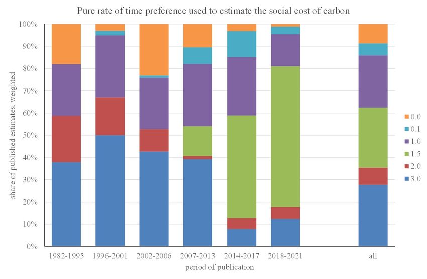
been mitigated to the point that its marginal impacts start to fall 8] 93 papers
estimate how fast, showing estimates of the social cost of carbon at two or more
points in time, for a total of 1,972 estimates of the growth rate of the social cost
of carbon.
I apply meta-analysis to these estimates. This is not the only way to make
the social cost of carbon more transparent. Sensitivity analysis[9] and model
comparison[10] are at least as insightful. Decomposition of model updates[11,
12] helps to understand the evolution of estimates, but only within the confines
of a single model. Only meta-analysis can show how the entire literature has
evolved over time.
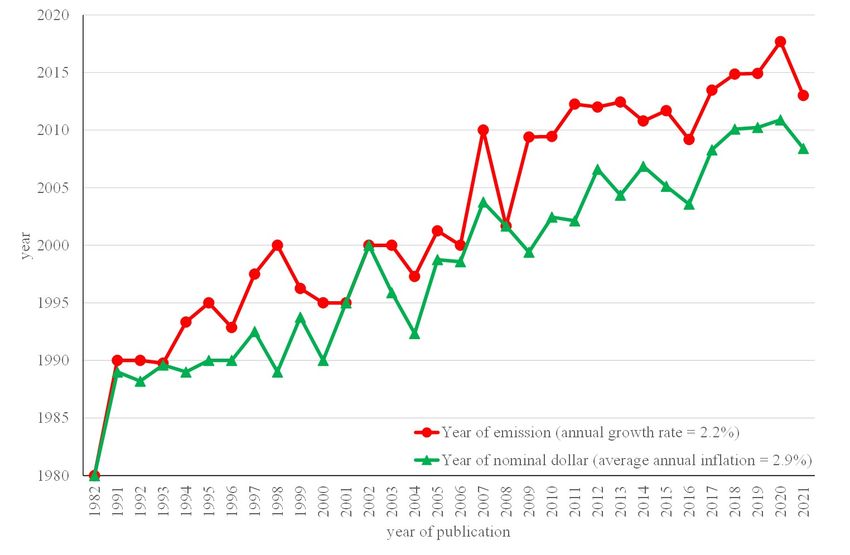
Figure 1 shows the mean and standard deviation of estimates of the social
cost of carbon by year of publication, as well as the standard error of the mean.
Table 1 show the mean and standard deviation by pure rate of time preference.
In this paper, estimates are expressed in 2010 US dollars per metric tonne
of carbon, and are for emissions in the year 2010. The literature uses nominal
dollars and a variety of emission years. See Figure S6. Particularly, later studies
report the social cost of carbon in later dollars for later emission years. Average
inflation was 2.9% over the period. The social cost of carbon grows by some
2.2% per year; this is the average across the 93 studies that estimate its growth
rate. Without correcting for emission year and inflation, the apparent trend in
the social cost of carbon equals 5.1% per year. After correction, some of the
early estimates are the highest. Between 1993 and 2008, estimates went up and
down without a discernible trend in either direction. Since 2009 or so, there
appears to be an increase in the social cost of carbon, and three of the last four
years stand out. An earlier meta-analysis finds that the social cost of carbon
has not increased over time[13] but a more recent one finds that it has[14]. The
mean for 2021 is higher than all but two other years; paired t-tests shows the
2021 mean is statistically significantly higher than all but four other years.
Everything about climate change is uncertain. An assessment of the liter-
ature of the social cost of carbon should reflect that uncertainty. Attention
should be paid to the entire probability distribution rather than just its central
tendency or its first and second moment. Figure 1 is incomplete.
Another problem with Figure 1 is that it invites an interpretation based on
the implicit assumption of normality. This is inappropriate. The uncertainty
about climate change is right-skewed.[15] This is the case for the uncertainty
about climate sensitivity.[16] Non-linear impact functions amplify higher-than-
expected warming over lower-than-expected climate change.[17] Risk aversion
emphasizes negative surprises over positive ones.[18] Any confidence interval
around the central estimate of the social cost of carbon is therefore asymmetric;
this message is lost by adding and subtracting the standard deviation or error
from the mean, as is done in Figure 1. The uncertainty about the social cost
of carbon is thick- or even fat-tailed.[19] The mean plus the standard deviation
does not equal the 83rd percentile. There is considerably more probability mass
outside the normal bounds. The t-tests referred to above may be overconfident.
If the distribution of the social cost of carbon is right-skewed and fat-tailed,
then recent estimates may well be within the historical range.
2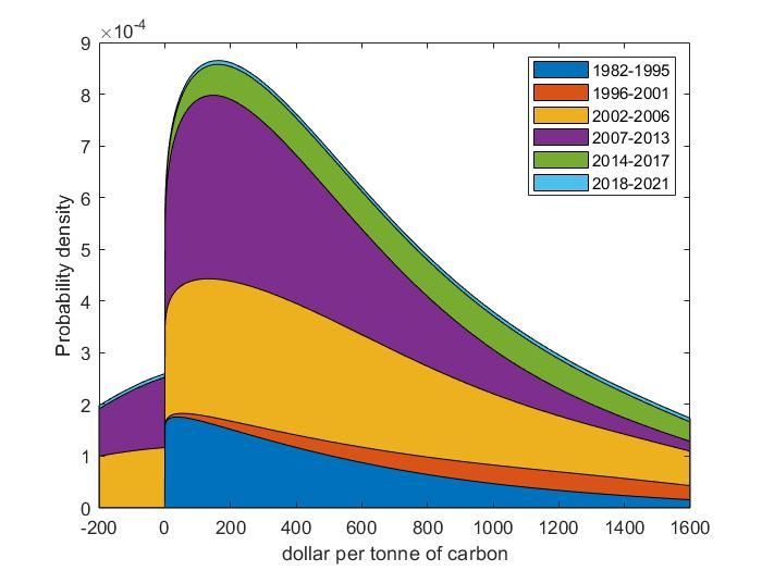
Standard probability density functions do not adequately describe the un-
certainty about the social cost of carbon, which is right-skewed and thick-
tailed. Kernel densities are a flexible alternative to parametric distribution
functions[20]. Kernel densities have been used to visualize the uncertainty
about the social cost of carbon.[21] I here add many more observations, and
decompose that uncertainty into discrete components, particularly publication
periods, testing whether the components differ from one another. Simple kernel
regression is helpful for specifying the relationship between two variables.[22]
Kernel quantile regression can be used to show this relationship across the dis-
tribution.[23] However, these methods are not suitable if the explanatory vari-
able is categorical—as is the case for discount rates or years of publication. The
method proposed here, kernel density decomposition, works for categorical data,
shows both central tendency and spread, and does not make assumptions about
functional form or the shape of the probability distribution.
    Kernel density decomposition therefore offer a more valid basis for statis-
tical tests than the paired t-tests above, which assume normality. In order to
test for changes over time, I split the sample into six periods, demarcated by
important events in the publication history of the social cost of carbon. These
key events are the Second Assessment Report of the Intergovernmental Panel on
Climate Change[24], the Third Assessment Report of the IPCC[25], the Stern
Review[26], the Obama update of the social cost of carbon[27], and the 2018
Nobel Memorial Prize in Economic Sciences.[28] These events reminded people
of the importance of pricing carbon and stimulated new research into the social
cost of carbon.
    The kernel density is estimated with bespoke kernel functions, reflecting
the deep and asymmetric uncertainty of the social cost of carbon. The data
are weighted for quality; implausibly high estimates are censored. The decom-
position of the kernel density is based on the fact that the weighted sum of
probability densities is a probability density.[29] The statistical test is that for
the equality of proportions.[30]. Applied to different publication periods, this is
a test for the stationarity of the distribution[31] of the social cost of carbon. See
Methods for the details, the Supplementary Information for sensitivity analyses.
    Figure 2 shows the kernel density of the social cost of carbon and its the
decomposition by publication period. The kernel density has the same shape
as the histogram in Figure S1: There is a little probability mass below zero,
a pronounced mode, and a thick right tail. Compared to the histogram, the
kernel density is smooth and spread wider. This is also seen in Table 1: Kernel
mean and standard deviation are larger than their empirical counterparts.
    Earlier studies exclude negative estimates, but other patterns are not ob-
vious from the kernel decomposition. Table S4 confirms this. It shows the
contributions of estimates of the social cost of carbon published in a particular
period to the overall kernel density and its quintiles. The quintile shares are
statistically indistinguishable from the overall shares; χ220 = 12.77; p = 0.887.
    This analysis only considers time. Figure S7 shows that the discount rate
used to estimate the social cost of carbon has varied over time. Particularly,
the once popular pure rate of time preference of 3.0% has been largely replaced

                                         3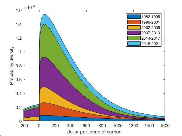
by 1.5%. This would increase the social cost of carbon. Table 1 and Figure S13
confirm this.
     Table 2 therefore repeats the analysis for the four pure rates of time prefer-
ence for which there are observations in every time period: 0%, 1%, 2% and 3%
(see Table S1). Conditional on the pure rate of time preference, the Equality of
Proportions test finds no statistically significant difference between the publica-
tion periods either. The Kolmogorov-Smirnov test finds the same for quintiles
but suggests differences at a finer resolution (see Table S9).
     Three more analyses are included in the Supplementary Material. These
analyses assume normality of error terms, avoiding the asymmetry and thick
tail that are a feature of the social cost of carbon but make upward trends
hard to detect. The first additional analysis is a weighted linear regression of
the social cost of carbon on the pure rate of time preference, which shows a
highly significant coefficient, and the year of publication, which is insignificant;
either result is independent of the weights used. See Table S14. In the second
analysis, the linear time trend is replaced by a flexible time trend. Again,
the effect of publication year is insignificant regardless of weights. See Figure
S12. Thirdly, quantile regression is used. The pure rate of time preference
is significant for almost all quantiles and weights; the year of publication for
almost none. However, the social cost of carbon appears to increase over time if
estimates are weighted for quality and attention is restricted to the central parts
of the distribution. See Table S14. All together, the upward trend in Figure 1
is not because of greater pessimism about climate change, but because analysts
have used lower discount rates.
     In sum, some have claimed that estimates of the social costs of carbon have
increased over time.[12, 32–34] There is an apparent upward trend because es-
timates are reported for later years, because of price inflation, and because
later analyses tend to use lower discount rates. Correcting for these factors and
properly accounting for the asymmetric, heavy-tailed uncertainty, there is no
statistically significant time trend in published estimates of the social cost of
carbon.
     The main reason for this null result is that the uncertainty about the social
cost of carbon is very large. Research continuously refines our knowledge and
updates our estimates, sometimes upwards, sometimes downwards. There are
still many things left to research[35] and left to improve in our estimates.[36, 37]
However, the social cost of carbon reflects the impact of future climate change
and the future is as uncertain now as it was then.
     The implication of the meta-analysis presented here is that the literature on
the social cost of carbon does not justify an upward revision of carbon prices
emission reduction targets. At the same time, the literature, summarized in
Table 1, suggests that, in most of the world, the price of carbon is too low.[38]
There is often a gap between the announced emissions targets and the policies
supposed to achieve the targets.[6] Instead of raising the social cost of carbon,
the recommended carbon price, attention should focus on raising the actual price
of carbon.

                                         4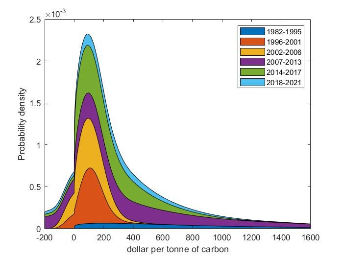
PRTP         empirical   kernel
                        3%              41         77
                                       (51)       (74)
                         2%            252        727
                                      (544)      (705)
                         1%            148        393
                                      (269)      (473)
                         0%            375        767
                                      (494)      (745)
                          all          177        502
                                      (377)      (550)

Table 1: Empirical and kernel average (standard deviation) of estimates of the
social cost of carbon by pure rate of time preference (PRTP).

                                            χ220      p
                      All                12.7726   0.8869
                      PRTP      =   0%    0.9577   1.0000
                      PRTP      =   1%    7.8782   0.9926
                      PRTP      =   2%   16.3455   0.6950
                      PRTP      =   3%   13.8335   0.8388

Table 2: Test for the equality of quintiles between publication periods for the
whole sample and for selected pure rates of time preference.

                                         5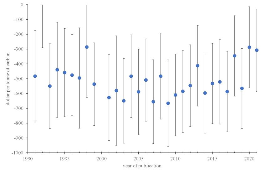
Figure 1: Average social cost of carbon by publication period. Outer error
bars are plus and minus the standard deviation of the published estimates,
inner error bars plus and minus the standard error of the mean. Estimates are
quality weighted and censored.

                                     6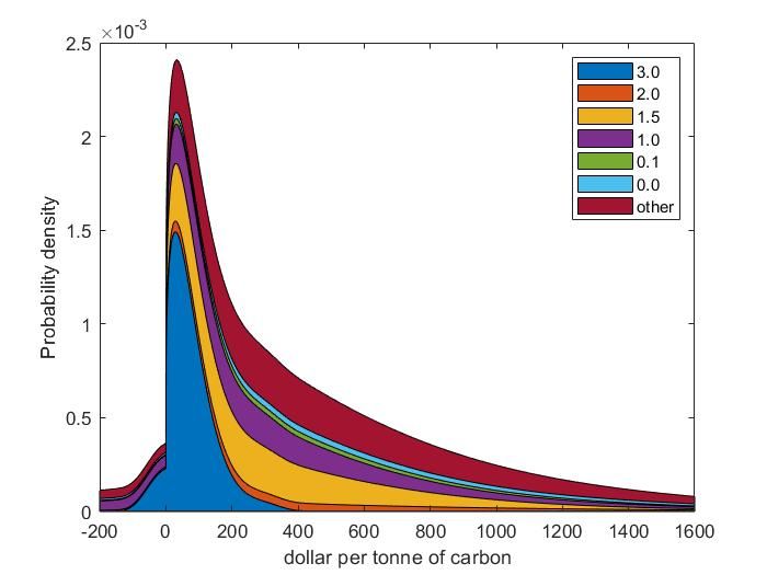
Figure 2: Kernel density of the social cost of carbon and its composition by
publication period.

                                     7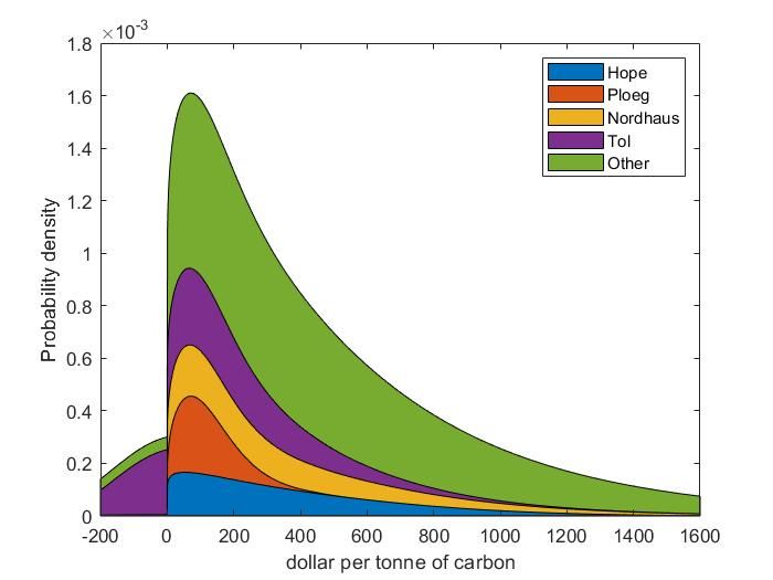
Methods
Kernel density decomposition
A kernel density is defined as
                                               n
                                          1 X             x − xi
                             f (x) =            K                                                  (1)
                                         nh i=1             h

where xi are a series of observations, h is the bandwidth, and K is the ker-
nel function. The kernel function is conventionally assumed to be a (i ) non-
negative (ii ) symmetric function that (iii ) integrates to one, with (iv )
zero mean and (v ) finite variance.[20] That is, any standardized symmetric
probability density function can serve as a kernel function. The Normal density
is a common choice.
    Conventions are just that. As long as the kernel function is non-negative (the
assumption of non-negativity is relaxed for bias reduction.[39]) and integrates
to one, an appropriately weighted sum of kernel functions is non-negative and
integrates to one—such a sum is a probability density function.[29, 40, 41]
    The kernel density is defined thus defined as the sum of probabilities; see
Equation (1). It is a vote-counting procedure[42] where the votes are uncertain.
This interpretation fits the nature of the data. Estimates of the social cost of
carbon are not “data” in the conventional sense of the word, nor can integrated
assessment models be seen as “data generating processes”. Besides, I use the
population of estimates rather than a sample. There is therefore no Frequentist
interpretation of the proposed method. There is no Bayesian interpretation
either. While we might take the kernel function to express degrees of belief, a
Bayesian procedure would take the first estimates[1] as prior and later estimates
as likelihoods, multiplying rather than adding probability densities.
    A kernel density can also be seen as a mixture density.[43, 44]. This reinter-
pretation opens a route to decomposition. We can construct the kernel density
of any subset of xi . The weighted sum of the kernel densities of the subsets is
a kernel density.
    With the right weights and bandwidths, the weighted sum of the kernel
densities of subsets of the data is identical to the kernel density of the whole
data Pset. To see this, partition the observations into m subsets of length mj
with j mj = n, as x1 , ...xm1 , xm1 +1 , ..., xm1 +m2 , xm1 +m2 +1 , ..., xn . Then
                                       Pj
                                            m
                   m
                   X mj     1           X k
                                        k=1
                                                              x − xi
                                                                               m
                                                                                X mj
         f (x) =                                      K                    =:             fj (x)   (2)
                   j=1
                         n mj h    Pj−1                         h               j=1
                                                                                      n
                                  i=          mk +1
                                        k=1

This is identical to Equation (1). Moreover, each of the components fj of the
composite kernel density f is itself a kernel density.
   Kernel decomposition works with any set of weights that add to one, and

                                                8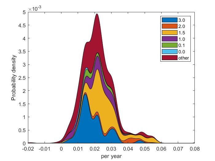
with any kernel function or bandwidth for the subsets:
                            Pj
                                  m
                Xm
                     wj       X k
                              k=1
                                           x − xi
                                                      Xm
        f (x) =                      Kj             =:     wj fj (x; hj )      (3)
                j=1
                    mj hj Pj−1               hj        j=1
                           i=         mk +1
                                k=1

In this case, the composite kernel density is not be the same as the kernel density
fitted to the complete data set. It is hard to argue for different kernel functions
Kj for different subsets of the data, but different subsets of the data would have
different spreads and hence bandwidths hj .

Inference
Equation (3) holds that the kernel density f (x) is composed of m kernel densities
fj (x) with weight mj /n. For each interval x < x < x̄, I test whether the shares
of the component densities equal its weight, using the Equality of Proportions
test.[30] Suppose, for example, that a component density makes up 17% of the
overall density. Then, the null hypothesis is that the left-tail, central part and
right-tail of the component density also make up 17% of the left-tail, central
part and right-tail of the overall density.
    Let intervals correspond to p percentiles of the composite distribution. The
test statistic is
                                          R                    2
                                             Pk+1            m
                                 n
                                   p X
                                   X   m
                                            P k
                                                  fj (x)dx − nj
                  χ2(m−1)(p−1) =                      mj                        (4)
                                 p    j=1              n
                                  k=0

The test only works if there are two components or more, m ≥ 2. If not, there
would be nothing to compare. The distribution needs to be split in two quantiles
or more, p ≥ 2, because each component density adds up to its weight mj /n by
construction. Again, there would be nothing to compare with fewer than two
quantiles.

References
  1.   Nordhaus, W. D. How Fast Should We Graze the Global Commons?
       American Economic Review 72, 242–246 (1982).
  2.   Pigou, A. The Economics of Welfare (Macmillan, London, 1920).
  3.   Pareto, V. Manuale di economia politica con una introduzione alla scienza
       sociale (Società Editrice Libraria, Milan, 1906).
  4.   Kaufman, N., Barron, A., Krawczyk, W., Marsters, P. & McJeon, H. A
       near-term to net zero alternative to the social cost of carbon for setting
       carbon prices. Nature Climate Change 10, 1010–1014 (2020).

                                              9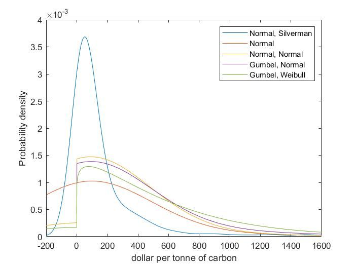
5.   Stern, N. & Stiglitz, J. E. The Social Cost of Carbon, Risk, Distribu-
      tion, Market Failures: An Alternative Approach Working Paper 28472
      (National Bureau of Economic Research, Feb. 2021). http://www.nber.
      org/papers/w28472.
 6.   UNFCCC. NDC Synthesis Report tech. rep. (United Nations Framework
      Convention on Climate Change Secretariat, Feb. 2021). https://unfccc.
      int / process - and - meetings / the - paris - agreement / nationally -
      determined-contributions-ndcs/nationally-determined-contributions-
      ndcs/ndc-synthesis-report.
 7.   Taconet, N., Guivarch, C. & Pottier, A. Social Cost of Carbon Under
      Stochastic Tipping Points. Environmental & Resource Economics. https:
      / / link . springer . com / article / 10 . 1007 / s10640 - 021 - 00549 - x
      (forthcoming).
 8.   van der Ploeg, F. & Withagen, C. Growth, Renewables, And The Optimal
      Carbon Tax. International Economic Review 55, 283–311 (2014).
 9.   Anthoff, D. & Tol, R. J. The uncertainty about the social cost of carbon:
      A decomposition analysis using FUND. Climatic Change 117, 515–530
      (2013).
10.   Diaz, D. & Moore, F. Quantifying the economic risks of climate change.
      Nature Climate Change 7, 774–782 (2017).
11.   Nordhaus, W. D. Evolution of modeling of the economics of global warm-
      ing: changes in the DICE model, 1992–2017. Climatic Change 148, 623–
      640 (2018).
12.   Hänsel, M. et al. Climate economics support for the UN climate targets.
      Nature Climate Change 10, 781–789 (2020).
13.   Havranek, T., Irsova, Z., Janda, K. & Zilberman, D. Selective reporting
      and the social cost of carbon. Energy Economics 51, 394–406 (2015).
14.   Wang, P., Deng, X., Zhou, H. & Yu, S. Estimates of the social cost of
      carbon: A review based on meta-analysis. Journal of Cleaner Production
      209, 1494–1507. http://www.sciencedirect.com/science/article/
      pii/S0959652618334589 (2019).
15.   Tol, R. S. J. The marginal costs of greenhouse gas emissions. Energy
      Journal 20, 61–81 (1999).
16.   Roe, G. H. & Baker, M. B. Why Is Climate Sensitivity So Unpredictable?
      Science 318, 629–632. https://science.sciencemag.org/content/
      318/5850/629 (2007).
17.   Nordhaus, W. D. An Optimal Transition Path for Controlling Greenhouse
      Gases. Science 258, 1315–1319 (1992).
18.   Anthoff, D., Tol, R. S. J. & Yohe, G. W. Risk aversion, time preference,
      and the social cost of carbon. Environmental Research Letters 4, 024002
      (2009).

                                      10
19. Weitzman, M. L. On Modeling and Interpreting the Economics of Catas-
trophic Climate Change. The Review of Economics and Statistics 91, 1–
19 (2009).
20. Takezawa, K. Introduction to Nonparametric Regression (John Wiley and
Sons, Hoboken, 2005).
21. Tol, R. S. J. The Economic Impacts of Climate Change. Review of Envi-
ronmental Economics and Policy 12, 4–25. https://doi.org/10.1093/
reep/rex027 (Jan. 2018).
22. Altman, N. An introduction to kernel and nearest-neighbor nonparamet-
ric regression. American Statistician 46, 175–185 (1992).
23. Yu, K. & Jones, M. Local linear quantile regression. Journal of the Amer-
ican Statistical Association 93, 228–237 (1998).
24. Pearce, D. W. et al. in Climate Change 1995: Economic and Social Di-
mensions – Contribution of Working Group III to the Second Assessment
Report of the Intergovernmental Panel on Climate Change (eds Bruce,
J. P., Lee, H. & Haites, E. F.) 179–224 (Cambridge University Press,
Cambridge, 1996).
25. Smith, J. B. et al. in Climate Change 2001: Impacts, Adaptation, and
Vulnerability (eds McCarthy, J. J., Canziani, O. F., Leary, N. A., Dokken,
D. J. & White, K. S.) 913–967 (Press Syndicate of the University of
Cambridge, Cambridge, UK, 2001).
26. Stern, N. H. et al. Stern Review: The Economics of Climate Change (HM
Treasury, London, 2006).
27. Interagency Working Group on the Social Cost of Carbon. Technical sup-
port document: Technical update of the social cost of carbon for regulatory
impact analysis under Executive Order 12866 Report (United States Gov-
ernment, 2013).
28. Nordhaus, W. Climate Change: The Ultimate Challenge for Economics.
American Economic Review 109, 1991–2014. https : / / www . aeaweb .
org/articles?id=10.1257/aer.109.6.1991 (June 2019).
29. Quetelet, A. Lettres à S. A. R. le Duc Régnant de Saxe-Cobourget Gotha,
sur la théorie des probabilités, appliquée aux sciences morales et politiques
(Hayez, Brussels, 1846).
30. Pearson, K. On the criterion that a given system of deviations from the
probable in the case of a correlated system of variables is such that it
can be reasonably supposed to have arisen from random sampling. The
London, Edinburgh, and Dublin Philosophical Magazine and Journal of
Science 50, 157–175. https://doi.org/10.1080/14786440009463897
(1900).
31. Andrews, I. & Kasy, M. Identification of and Correction for Publication
Bias. American Economic Review 109, 2766–94. https://www.aeaweb.
org/articles?id=10.1257/aer.20180310 (Aug. 2019).
1132. Van Den Bergh, J. & Botzen, W. A lower bound to the social cost of CO2
emissions. Nature Climate Change 4, 253–258 (2014).
33. Base the social cost of carbon on the science. Nature 541, 260 (2017).
34. Wagner, G. Recalculate the social cost of carbon. Nature Climate Change
11, 293–294 (2021).
35. Burke, M. et al. Opportunities for advances in climate change economics.
Science 352, 292–293 (2016).
36. NAS. Valuing climate damages: Updating estimation of the social cost of
carbon dioxide 1–262 (National Academies of Sciences, Engineering, and
Medicine, Washington, D.C., 2017).
37. Wagner, G. et al. Eight priorities for calculating the social cost of carbon.
Nature 590, 548–550 (2021).
38. ICAP. Allowance Price Explorer tech. rep. (International Carbon Action
Partnership, Apr. 2021). https : / / icapcarbonaction . com / en / ets -
prices.
39. Jones, M. & Signorini, D. A comparison of higher-order bias kernel density
estimators. Journal of the American Statistical Association 92, 1063–1073
(1997).
40. Quetelet, A. Sur quelques propriétés curieuses que présentent les résultats
d’une serie d’observations, faites dans la vue de déterminer une constante,
lorsque les chances de rencontrer des écarts en plus et en moins sont égales
et indépendantés les unes des autres. Bulletins de l’Académie royale des
sciences, des lettres et des beaux-arts de Belgique 19 (2), 303–317 (1852).
41. Pearson, K. III. Contributions to the mathematical theory of evolution.
Philosophical Transactions of the Royal Society of London. (A.) 185, 71–
110. https://royalsocietypublishing.org/doi/abs/10.1098/rsta.
1894.0003 (1894).
42. Laplace, P.-S. Essai philosophique sur les probabilités (Ve Courcier, Paris,
1814).
43. Makov, U. in International Encyclopedia of the Social & Behavioral Sci-
ences (eds Smelser, N. J. & Baltes, P. B.) 9910–9915 (Pergamon, Oxford,
2001). isbn: 978-0-08-043076-8.
44. McLachlan, G. & Peel, D. Finite Mixture Models (John Wiley and Sons,
Hoboken, 2001).
12Supplementary materials: Data and methods
Papers used in the meta-analysis
The database draws on earlier meta-analyses of the social cost of carbon,[1–6]
extended with recent papers that were found using search engines and a review
of the publication records of active researchers. 201 papers were used.[7–207]
The record is close to complete for papers published before April 2021.
Most of the papers report results in tabular format. Some only show results
in graphs, but most authors emailed the underlying data upon request; if not,
the Matlab routine grabit[208] was used to digitize the graphs.
The meta-analysis uses the estimate of the social cost of carbon, the year
of emission, the year of the nominal dollar, the year of publication, the author,
weights, censoring, and the pure rate of time preference. These data, plus some
not used here, can be found on GitHub.
Descriptive statistics
Table S1 shows the number of estimates per publication period and discount
rate, and the number of papers per period. Three papers are counted double
because they present comparative results of two different models. There is an
upward trend in the number of papers per period, and in the number of estimates
per paper.
Table S2 shows the mean and standard deviation of the estimates of the
social cost of carbon by publication period and year. The range of estimates
has grown very wide in recent years.
Figure S1 shows the histogram of the published estimates of the social cost
of carbon, using quality weights and censoring (see below). Some estimates are
negative, a social benefit of carbon, but the vast majority is positive. The mode
lies between 0 and $50/tC, but there is a long right tail. The 95th percentile is
$800/tC.
Bandwidth and kernel function
The choice of kernel function and bandwidth is key to any kernel density esti-
mate, as illustrated in Figure S2. If kernel density estimation is interpreted as
vote-counting, kernel and bandwidth should be chosen to reflect the nature of
the data, shown in Figure S1. In this case, the uncertainty about the social cost
of carbon is large and right-skewed. Furthermore, the social cost of carbon is,
most researchers argue, a cost and not a benefit.
A conventional choice would be to use a Normal kernel function, with a
bandwidth according to the Silverman rule[209], that is, 1.06 times the sample
standard deviation divided by the fifth root of the number of observations.
Figure S2 reveals two problems with this approach: The right tail of the resulting
kernel density is thin, and a large probability mass is assigned to negative social
costs of carbon. If the bandwidth equals the sample standard deviation to reflect
S1the wide uncertainty, the right tail appropriately thickens but the probability
of a Pigou subsidy on greenhouse gas emissions increases too.
Many of the published estimates of the social cost of carbon are based on an
impact function that excludes benefits of climate change. Climate change can
only do damage and additional carbon dioxide can only be bad. Honouring that,
I assign a knotted Normal kernel function to these observations. As the kernel
function is asymmetric, centralization needs to be carefully considered—is xi
in Equation (1) the mean, median or mode of K? I prefer to use the mode as its
central tendency, in line with the interpretation of kernel density estimation as
vote-counting (see below). With these assumptions, Figure S2 shows that the
probability of a negative social cost of carbon falls.
The studies that report the possibility of a negative social cost of carbon
nonetheless argue in favour of a positive one. A symmetric Normal kernel does
not reflect that. I therefore replace it with a Gumbel kernel:
1 x−µ x−µ
f (x) = exp − − exp − (S1)
β β β
The Gumbel distribution is defined on the real line but right-skewed. Again, I
use the mode µ as its central tendency. This thickens the right tail and thins
the left tail.
A knotted Normal kernel is not only peculiar near zero but it also has a thin
tail. I therefore replace it with a Weibull kernel:
κ x κ−1 x κ
f (x) = exp (S2)
λ λ λ
The Weibull is defined on the positive real line, f (x) is near zero if x is near
1/κ
zero, and right-skewed. I use the mode λ (κ − 1/κ) as its central tendency. The
right tail of the kernel distribution thickens again. The Weibull-Gumbel kernel
distribution is the default used here.
The Matlab code can be found on GitHub.
Weights
The social cost of carbon is an estimate of the willingness to pay to reduce carbon
dioxide emissions. Willingness to pay is limited by ability to pay. 282 out of
5,397 estimates violate this. If the estimated social cost of carbon were levied
as a carbon tax, tax revenue would exceed total income. This is not possible.
These estimates, exceeding $7,609/tC (the global average carbon intensity in
2010), are excluded.
Another 1,186 estimates are so large that, if levied as a carbon tax, the
public sector would grow beyond its global average of 15% in 2010, even if
all other taxes would be abolished. Estimates in excess of this Leviathan
tax[210], $1,141/tC, are discounted. The discount is linear, varying between
0 for $1,141/tC and 1 for $7,609/tC. Without these discounts, very large esti-
mates of the social cost of carbon dominate the analysis; cf. Table S2.
S2The estimates of the social cost of carbon are weighted in three different
ways. First, all estimates are treated equally. This is graph “no weights” in
Figure S3. While some papers present a single estimate of the social cost of
carbon, other papers show many, up to 1,229 variants[207]. This emphasizes
studies that ran many sensitivity analyses, which became easier as computers
got faster. Secondly, estimates are weighted such that the total weight per paper
equals one. This is “paper weights” in Figure S3. Within each paper, estimates
that are favoured by the authors are given higher weight. Favoured estimates
are highlighted in the abstract and conclusions, and they are used as the starting
point in robustness checks. Estimates that are shown in order to demonstrate
that the new model can replicate earlier work are not favoured. This is “author
weights” in Figure S3.
Different experts have cast different numbers of votes. I count one paper
as one vote. One can also argue that it should be one vote per expert, or that
papers should be weighted by citations, journal prestige, or author pedigree.
Composite kernel densities naturally allow for this, but it is a dangerous route
to travel in this case. Older papers are cited more than younger papers; journal
rankings are hard enough within disciplines, harder still between disciplines;
and prestige, reputation and pedigree often reflect old glory rather than current
wits.
Instead, I use a set of weights that reflect the quality of the paper. Over
95% of the estimates are peer-reviewed; these score 1; the rest score 0. Almost
95% use an emission scenario; these score 1; papers based on arbitrary emissions
score 0 as do papers assuming a steady state. Almost 99% of estimates estimate
the social cost of carbon as a true marginal or a small increment; these score 1;
papers with ropy mathematics score 0 as do papers reporting an average rather
than a marginal. Over 68% of estimates assume that vulnerability to climate
change is constant; these score 0; papers that recognize that the impacts of
climate change vary with development score 1. Only 3% of estimates is based
on new estimates of the total impact of climate change; these score 1; the rest
score 0. These scores are added. This is “quality weights” in Figure S3.
Figure S3 shows the impact of the weights. The censoring of large estimates,
in excess of the Leviathan tax or even in excess of income, has the largest effect.
The maximum estimate in the data is $107,260,751/tC. Including estimates like
these, the kernel bandwidth becomes so large that the kernel density becomes
almost uniform.
The censored data reveal an articulated probability density function. The
unweighted estimates have the fattest tail; that is, papers that are more pes-
simistic about climate change present more estimates of the social cost of carbon.
Giving every paper, rather than every estimate, a unit weight thins the right
tail. Discounting estimates that their own authors discount further thins the
tail. This result is mechanical, as the convention in sensitivity analysis is to show
both high and low alternatives to the central assumptions. Quality weights thin
the tail further still. More credible studies are less pessimistic.
S3Uncertainty about uncertainty
The kernel density describes the uncertainty about the social cost of carbon.
The kernel density is an estimate and as such uncertain. Above and below, I
ignore the uncertainty about the uncertainty. Figure S4 shows the 95% con-
fidence interval around the Weibull-Gumbel kernel distribution of Figure S2,
using quality weights as in Figure S3. This confidence interval is based on a
bootstrap of 1,000 replications of the published estimates (without reweighing).
The shape of the kernel distribution is well-defined. The key uncertainty is
about the weight of the tail relative to the central part of the distribution.
Ignoring the uncertainty about the uncertainty makes it more likely to detect
patterns. As I find that the primary uncertainty is too large to detect changes
over time, ignoring secondary uncertainty does not affect the results. I there-
fore proceed without the computationally expensive bootstrap and without the
conceptually challenging meta-uncertainty.
Publication bias
Publication bias in the literature on the social cost of carbon has been reported
[211]. Standard tests for publication bias are designed for statistical analyses,
particularly test for a reluctance to publish insignificant results. The reported
“publication bias” thus reflects that few studies report negative estimates of the
social cost of carbon. Indeed, in the original DICE model [14], the social cost
of carbon is positive by construction (see above). Many later papers follow in
Nordhaus’ footsteps. The reported publication bias is perhaps better interpreted
as confirmation bias.
A recently proposed test for publication bias[212] is more general and can be
applied to non-statistical results. The null hypothesis is that earlier and later
studies are drawn from the same distribution. If not, later studies are influenced
by earlier results—a sign of publication bias. The test used here is similar in
spirit—does the distribution change over time—but the interpretation is about
the knowledge base rather than the publication practice. It is not possible to
disentangle changes in knowledge from changes in publication.
S4Supplementary materials: Results
The growth rate of the social cost of carbon
Different studies report the social cost of carbon for different years of emission.
Estimates are standardized to emissions in the year 2010, assuming that the
social cost of carbon grows by some 2.2% per year. That is, estimates for 2000,
say, are multiplied by 1.02210 and estimates for 2020 are divided by the same
factor. This correction factor is the same for all studies and for all estimates.
Figure S5 shows the kernel density of the growth rate of the social cost
of carbon, decomposed for the pure rate of time preference. The density is
symmetric for a 3.0% utility discount rate. However, for discount rates of 1.5%
and 2.0%, little probability mass is added to the left tail, and a lot to the right
tail.
Table S3 shows the shares by quintile of the kernel density. The same pattern
is seen as in the graph, but Pearson’s test does not reject the null hypothesis that
the component densities are equal to the composite one; χ224 = 3.50; p = 1.000.
This justifies the assumption of a uniform growth rate of the social cost of
carbon.
Time and discount
Table S4 and Figure 2 show that the distribution of the social cost of carbon has
not significantly changed over time. Figure S7, however, reveals that the pure
rate of time preference used to estimate the social cost of carbon has changed
over time. Notably, a 1.5% pure rate of time preference was first used in 2011
and became the dominant choice in later years.
I therefore redo the decomposition per period for four alternative pure rates
of time preference, 0%, 1%, 2%, and 3%, which have been used throughout the
period. Tables S5, S6, S7 and S8 and Figures S8, S9, S10 and S11 show the
detailed results, Table 2 the summary. The null hypothesis that the six periods
show the same probability density function for the social cost of carbon cannot
be rejected regardless of the choice of pure rate of time preference.
Alternative non-parametric tests
Pearson’s equality of proportions test is designed to compare the distributions
of subsamples to the distribution of the whole sample. Alternatively, the sub-
sample distributions can be scaled up to sum to one, and tests for the equality
of distributions can be applied. However, for most of these tests, critical values
are tabulated for specific null hypotheses only. These tests can be use to check
whether the subsample distribution is, say, Normal but not whether it conforms
to the whole-sample kernel distribution. The Kolmogorov-Smirnov test is the
exception: Its test statistic converges to a known distribution, independent of
the null hypothesis.[213] I did not use the tabulations.[214], instead computed
the p-values.[215] Pearson’s Equality of Proportions test considers the difference
S5between entire distributions. The Kolmogorov-Smirnov test, on the other hand,
consider the maximum deviation between distributions.
Table S9 shows the results. The null hypothesis that the quintiles of the
subperiod distributions are equal to the quintiles of the distribution of the whole
period, cannot be rejected. The equality of proportions test was applied to
quintiles too. The two statistical tests agree.
The null hypothesis cannot be rejected for deciles and ventiles either. How-
ever, the null hypothesis is rejected for the third period if quinquagintiles are
considered. For centiles, the null hypothesis is rejected for the first and third
periods, and almost for the fourth and sixth. That is, the subperiod distribu-
tions are indistinguishable at a crude resolution but differences appear at a finer
scale.
Tables S10 to S13 repeat the analysis, splitting the sample by discount rate
and time period. Rejections of the null hypothesis are common, also for quintiles
and deciles. However, Table S1 reveals that cell-sizes can be small, down to
five estimates. With so few observations, confidence in the estimated kernel
densities is low. Nonetheless, the more discerning Kolmogorov-Smirnov test
points to changes over time that the Pearson test cannot detect.
Parametric tests
Table S14 shows the results for the weighted linear regression, based on the
conventional assumptions of linearity and normality, of the social cost of carbon
on the pure rate of time preference and the year of publication, using paper,
author and quality weights. The time trend is not statistically significant from
zero.
I repeat the analysis using year fixed effects rather than a linear time trend.
Figure S12 shows the estimated time dummies, measuring the deviation from
1982. The dummies do not show a trend.
Table S14 also shows the results of quantile regressions, for quintiles as
above. The time trend is insignificant for paper and author weights. Using
quality weights, the time trend is positive and significant at the 5% level for the
three lower quintiles. That is, lower estimates of the social cost of carbon are
gradually disappearing from the higher-quality literature.
Discount rate
The social cost of carbon is the net prevent value of the additional future dam-
ages done by emitting slightly more carbon dioxide. The assumed discount rate
is obviously important in its calculation.
Figure S13 decomposes the kernel density of the social cost of carbon into
its components by pure rate of time preference used. “Other” refers to a range
of numbers and methods, including constant consumption rates, various forms
of declining discount rates, and Epstein-Zin preferences. As one would expect,
the lower discount rates contribute more to the right tail of the distribution.
S6Table S15 shows the contributions of estimates of the social cost of carbon
using a particular pure rate of time preference to the overall kernel density
(denoted ”null”) as well as to the five quintiles of that density (denoted Q1-5).
The null hypothesis that all shares are equal is firmly rejected; χ224 = 50.69; p =
0.001.
This result justifies splitting the sample by discount rate. It also demon-
strates that the Pearson test for the Equality of Proportions has the power to
reject null hypotheses for these data and these kernel densities.
Author
I also test whether different researchers reach different conclusions, one test of
the impact of subjective judgements on estimates of the social cost of carbon.
The decomposition of the kernel density by author opens another interpre-
tation of kernel densities: Vote-counting.[216] Different experts have published
different estimates of the social cost of carbon. These can be seen as votes for
a particular Pigou tax. But as the experts are uncertain, they have voted for
a central value and a spread. The kernel function is a vote, the kernel density
adds those votes. Note the difference with Bayesian updating, which multiplies
rather than adds probabilities.
I spit the sample into estimates by those who have published ten papers
or more (i.e., Christopher W. Hope, William D. Nordhaus, Frederick van der
Ploeg, Richard S.J. Tol) and others.
Figure S14 decomposes the kernel density by author. Of the named authors,
estimates by van der Ploeg are the narrowest, Tol contributes most to the left
tail, and Hope to the right tail.
Table S16 shows the contributions of estimates of the social cost of carbon
published by a particular author to the overall kernel density and its quintiles.
There are patterns in figure and table, and the null hypothesis that the quintile
shares are indistinguishable from the overall shares cannot be rejected; χ216 =
20.42; p = 0.202.
This justifies that the sample is split by period and discount rate, rather
than by period, discount rate, and author.
1982-1995 1996-2001 2002-2006 2007-2013 2014-2017 2018-2021 total
3.0% 33 27 39 108 24 106 337
2.0% 5 7 14 7 139 313 485
1.5% 0 0 0 38 216 1679 1933
1.0% 8 16 28 100 190 448 790
0.1% 0 4 1 21 69 121 216
0.0% 68 5 33 43 124 262 535
other 12 25 26 317 287 828 1495
# estimates 126 84 141 634 1049 3757 5791
# papers 19 18 23 51 52 41 204
Table S1: Number of papers on the social cost of carbon by publication period
and the number of estimates by period and pure rate of time preference.
S71982-1995 1996-2001 2002-2006 2007-2013 2014-2017 2018-2021 all
3.0% 23 65 25 25 53 131 43
(14) (88) (24) (17) (27) (50) (53)
2.0% 37 53 66 124 179 1042 220
(18) (26) (47) (113) (144) (1212) (588)
1.5% 205 1659 11328 6350
(560) (12318) (388584) (275486)
1.0% 439 92 100 181 186 13704 1980
(409) (57) (112) (370) (980) (158497) (57875)
0.1% 552 575 331 440 466 417
(325) (439) (1265) (953) (988)
0.0% 408 867 448 385 1608 1509 561
(746) (439) (548) (1102) (3083) (2903) (1313)
other 1010 466 119 162 184 28025 5067
(1725) (659) (112) (178) (332) (1318717) (548248)
all 392 217 143 158 631 14454 3177
(994) (433) (297) (395) (6553) (744232) (333710)
Table S2: Average (standard deviation) of estimates of the social cost of carbon
by publication period and pure rate of time preference.
3.0 2.0 1.5 1.0 0.1 0.0 other
Q1 0.0696 0.0012 0.0129 0.0188 0.0050 0.0101 0.0789
Q2 0.0751 0.0040 0.0346 0.0172 0.0113 0.0023 0.0582
Q3 0.0416 0.0048 0.0647 0.0204 0.0053 0.0006 0.0615
Q4 0.0251 0.0056 0.0875 0.0244 0.0084 0.0011 0.0483
Q5 0.0323 0.0224 0.0780 0.0216 0.0067 0.0021 0.0388
Null 0.0487 0.0076 0.0555 0.0205 0.0073 0.0032 0.0571
Table S3: Observed and hypothesized contribution to the kernel density of
the growth rate of the social cost of carbon by quintile and pure rate of time
preference.
1982-1995 1996-2001 2002-2006 2007-2013 2014-2017 2018-2021
Q1 0.0086 0.0231 0.0365 0.0829 0.0566 0.0224
Q2 0.0126 0.0266 0.0298 0.0643 0.0704 0.0241
Q3 0.0135 0.0238 0.0231 0.0595 0.0624 0.0271
Q4 0.0156 0.0194 0.0152 0.0488 0.0491 0.0317
Q5 0.0295 0.0140 0.0068 0.0267 0.0260 0.0496
Null 0.0160 0.0214 0.0223 0.0564 0.0529 0.0310
Table S4: Observed and hypothesized contribution to the kernel density by
quintile and publication period.
S81982-1995 1996-2001 2002-2006 2007-2013 2014-2017 2018-2021
Q1 0.0286 0.0016 0.0880 0.0943 0.0082 0.0043
Q2 0.0380 0.0060 0.0756 0.0913 0.0198 0.0022
Q3 0.0294 0.0105 0.0733 0.0676 0.0252 0.0028
Q4 0.0220 0.0178 0.0653 0.0394 0.0314 0.0039
Q5 0.0119 0.0201 0.0553 0.0167 0.0325 0.0173
Null 0.0260 0.0112 0.0715 0.0618 0.0234 0.0061
Table S5: Observed and hypothesized contribution to the kernel density by
quintile and publication period, for a pure rate of time preference of 0%.
1982-1995 1996-2001 2002-2006 2007-2013 2014-2017 2018-2021
Q1 0.0028 0.0332 0.0517 0.0802 0.0430 0.0198
Q2 0.0094 0.0833 0.0764 0.0450 0.0795 0.0201
Q3 0.0115 0.0170 0.0219 0.0482 0.0628 0.0199
Q4 0.0150 0.0008 0.0019 0.0548 0.0417 0.0181
Q5 0.0277 0.0000 0.0001 0.0862 0.0145 0.0137
Null 0.0133 0.0269 0.0304 0.0629 0.0483 0.0183
Table S6: Observed and hypothesized contribution to the kernel density by
quintile and publication period, for a pure rate of time preference of 1%.
1982-1995 1996-2001 2002-2006 2007-2013 2014-2017 2018-2021
Q1 0.1510 0.2672 0.2229 0.0236 0.0785 0.0099
Q2 0.0000 0.0007 0.0071 0.0172 0.0856 0.0088
Q3 0.0000 0.0000 0.0000 0.0047 0.0377 0.0123
Q4 0.0000 0.0000 0.0000 0.0001 0.0034 0.0194
Q5 0.0000 0.0000 0.0000 0.0000 0.0007 0.0492
Null 0.0302 0.0536 0.0460 0.0091 0.0412 0.0199
Table S7: Observed and hypothesized contribution to the kernel density by
quintile and publication period, for a pure rate of time preference of 2%.
1982-1995 1996-2001 2002-2006 2007-2013 2014-2017 2018-2021
Q1 0.0587 0.0213 0.0621 0.1077 0.0055 0.0029
Q2 0.0725 0.0279 0.0760 0.1518 0.0120 0.0026
Q3 0.0149 0.0299 0.0500 0.0767 0.0203 0.0050
Q4 0.0001 0.0351 0.0147 0.0124 0.0165 0.0099
Q5 0.0000 0.0796 0.0022 0.0018 0.0016 0.0282
Null 0.0293 0.0387 0.0410 0.0701 0.0112 0.0097
Table S8: Observed and hypothesized contribution to the kernel density by
quintile and publication period, for a pure rate of time preference of 3%.
S95 10 20 50 100
1982-1995 0.9984 0.9267 0.5850 0.0992 0.0049
1996-2001 1.0000 1.0000 0.9980 0.8388 0.4276
2002-2006 0.9833 0.7891 0.3586 0.0282 0.0004
2007-2013 1.0000 0.9950 0.8779 0.3460 0.0599
2014-2017 1.0000 0.9991 0.9466 0.4962 0.1269
2018-2021 1.0000 0.9968 0.8981 0.3828 0.0752
Table S9: p-values of Kolmogorov-Smirnov test statistic for the equality of the
distributions of the period subsample and the whole sample (rows) for different
discretizations of the distribution (columns).
5 10 20 50 100
1982-1995 0.9372 0.5978 0.1876 0.0054 0.0000
1996-2001 0.2169 0.0177 0.0002 0.0000 0.0000
2002-2006 0.2562 0.0282 0.0004 0.0000 0.0000
2007-2013 1.0000 1.0000 0.9999 0.9427 0.6196
2014-2017 0.9991 0.9360 0.6172 0.1128 0.0063
2018-2021 1.0000 1.0000 1.0000 0.9978 0.9155
Table S10: p-values of Kolmogorov-Smirnov test statistic for the equality of
the distributions of the period subsample and the whole sample (rows) for dif-
ferent discretizations of the distribution (columns), for a 0% pure rate of time
preference.
5 10 20 50 100
1982-1995 0.0009 0.0000 0.0000 0.0000 0.0000
1996-2001 0.0149 0.0000 0.0000 0.0000 0.0000
2002-2006 0.0149 0.0000 0.0000 0.0000 0.0000
2007-2013 0.1957 0.0133 0.0001 0.0000 0.0000
2014-2017 0.3288 0.0589 0.0015 0.0000 0.0000
2018-2021 0.7425 0.3145 0.0482 0.0002 0.0000
Table S11: p-values of Kolmogorov-Smirnov test statistic for the equality of
the distributions of the period subsample and the whole sample (rows) for dif-
ferent discretizations of the distribution (columns), for a 1% pure rate of time
preference.
S105 10 20 50 100
1982-1995 0.0009 0.0000 0.0000 0.0000 0.0000
1996-2001 0.0149 0.0000 0.0000 0.0000 0.0000
2002-2006 0.0149 0.0000 0.0000 0.0000 0.0000
2007-2013 0.1957 0.0133 0.0001 0.0000 0.0000
2014-2017 0.3288 0.0589 0.0015 0.0000 0.0000
2018-2021 0.7425 0.3145 0.0482 0.0002 0.0000
Table S12: p-values of Kolmogorov-Smirnov test statistic for the equality of
the distributions of the period subsample and the whole sample (rows) for dif-
ferent discretizations of the distribution (columns), for a 2% pure rate of time
preference.
5 10 20 50 100
1982-1995 0.1995 0.0139 0.0001 0.0000 0.0000
1996-2001 0.9820 0.7568 0.3260 0.0218 0.0002
2002-2006 0.6867 0.2456 0.0303 0.0001 0.0000
2007-2013 0.4337 0.1078 0.0048 0.0000 0.0000
2014-2017 0.9998 0.9249 0.5714 0.0876 0.0034
2018-2021 0.3940 0.0829 0.0032 0.0000 0.0000
Table S13: p-values of Kolmogorov-Smirnov test statistic for the equality of
the distributions of the period subsample and the whole sample (rows) for dif-
ferent discretizations of the distribution (columns), for a 3% pure rate of time
preference.
S11weight percentile PRTP year
paper -131*** (27) -3.38 (3.64)
0.1 -8.51** (3.53) 0.457 (0.501)
0.3 -17.3** (7.6) 0.541 (1.074)
0.5 -35.3*** (10.1) 0.866 (1.428)
0.7 -75.3** (32.1) 0.509 (4.557)
0.9 -175 (161) -2.05 (22.79)
author -133*** (28) -3.05 (3.54)
0.1 -8.81** (3.89) 0.643 (0.532)
0.3 -15.7** (7.3) 0.762 (0.995)
0.5 -33.7*** (8.9) 1.05 (1.21)
0.7 -71.4** (28.0) 0.791 (3.822)
0.9 -179 (184) -1.72 (25.17)
quality -104*** (16) -0.0936 (2.1011)
0.1 -7.41*** (1.86) 0.558** (0.234)
0.3 -9.97*** (2.48) 1.17*** (0.34)
0.5 -33.0*** (3.8) 1.18** (0.514)
0.7 -62.0*** (10.4) 0.966 (1.419)
0.9 -136*** (34) 4.36 (4.56)
Table S14: Results of weighted least squares and weighted quantile regression of
the social cost of carbon on the pure rate of time preference and the publication
year.
Standard errors are reported in brackets. Coefficients marked with ***, ** or * are statistically
significant at the 1%, 5% or 10% level, respectively. The top row has results for the mean
regression, the next five rows for the quantile regression for the indicated percentile.
3.0 2.0 1.5 1.0 0.1 0.0 other
Q1 0.1461 0.0065 0.0354 0.0435 0.0048 0.0082 0.0511
Q2 0.0494 0.0089 0.0486 0.0350 0.0055 0.0063 0.0490
Q3 0.0043 0.0093 0.0448 0.0336 0.0063 0.0076 0.0547
Q4 0.0001 0.0103 0.0382 0.0295 0.0074 0.0101 0.0630
Q5 0.0000 0.0168 0.0246 0.0240 0.0094 0.0204 0.0872
Null 0.0400 0.0103 0.0383 0.0331 0.0067 0.0105 0.0610
Table S15: Observed and hypothesized contribution to the kernel density by
quintile and pure rate of time preference.
S12Hope Nordhaus Ploeg Tol Other
Q1 0.0185 0.0270 0.0205 0.0740 0.0882
Q2 0.0234 0.0261 0.0276 0.0405 0.1063
Q3 0.0212 0.0036 0.0247 0.0297 0.1120
Q4 0.0185 0.0000 0.0216 0.0163 0.1201
Q5 0.0094 0.0000 0.0176 0.0048 0.1485
Null 0.0182 0.0114 0.0224 0.0331 0.1150
Table S16: Observed and hypothesized contribution to the kernel density by
quintile and author.
Figure S1: Histogram of the social cost of carbon. Results are quality-weighted
and censored.
S13Figure S2: Kernel density of the social cost of carbon for alternative kernel
functions and bandwidths.
S14Figure S3: Kernel density of the social cost of carbon for alternative weights.
S15Figure S4: The 95% confidence interval of the kernel density of the social cost
of carbon.
S16Figure S5: Kernel density of the growth rate of the social cost of carbon and its
composition by discount rate.
S17Figure S6: Year of emission and year of nominal dollar by year of publication.
Estimates are weighted such that every published paper counts equally.
S18Figure S7: The pure rate of time preference used to estimate the social cost of
carbon by publication period. Estimates are weighted such that every published
paper counts equally.
S19Figure S8: Kernel density of the social cost of carbon and its composition by
publication period,for a pure rate of time preference of 0%.
S20Figure S9: Kernel density of the social cost of carbon and its composition by
publication period,for a pure rate of time preference of 1%.
S21Figure S10: Kernel density of the social cost of carbon and its composition by
publication period,for a pure rate of time preference of 2%.
S22Figure S11: Kernel density of the social cost of carbon and its composition by
publication period,for a pure rate of time preference of 3%.
S23Figure S12: Year fixed-effects from a regression of the social cost of carbon on
the pure rate of time preference, using quality weights. Base year is 1992; results
for 1991 are not shown; error bars denote the 67% confidence interval.
S24Figure S13: Kernel density of the social cost of carbon and its composition by
the pure rate of time preference.
S25Figure S14: Kernel density of the social cost of carbon and its composition by
author.
S26Additional references
1. Tol, R. S. J. The marginal damage costs of carbon dioxide emissions:
an assessment of the uncertainties. Energy Policy 33, 2064–2074. issn:
0301-4215 (2005).
2. Tol, R. S. J. The Economic Effects of Climate Change. Journal of Eco-
nomic Perspectives 23, 29–51. https://www.aeaweb.org/articles?
id=10.1257/jep.23.2.29 (June 2009).
3. Tol, R. S. J. The Economic Impact of Climate Change. Perspektiven der
Wirtschaftspolitik 11, 13–37. https://onlinelibrary.wiley.com/doi/
abs/10.1111/j.1468-2516.2010.00326.x (2010).
4. Tol, R. S. J. The Social Cost of Carbon. Annual Review of Resource
Economics 3, 419–443. https://doi.org/10.1146/annurev-resource-
083110-120028 (2011).
5. Tol, R. S. J. Targets for global climate policy: An overview. Journal of
Economic Dynamics and Control 37, 911–928. issn: 0165-1889. https://
www.sciencedirect.com/science/article/pii/S0165188913000092
(2013).
6. Tol, R. S. J. The Economic Impacts of Climate Change. Review of Envi-
ronmental Economics and Policy 12, 4–25. https://doi.org/10.1093/
reep/rex027 (Jan. 2018).
7. Nordhaus, W. D. How Fast Should We Graze the Global Commons?
American Economic Review 72, 242–246 (1982).
8. Ayres, R. & Walter, J. The greenhouse effect: Damages, costs and abate-
ment. Environmental & Resource Economics 1, 237–270 (1991).
9. Nordhaus, W. D. To Slow or Not to Slow: The Economics of the Green-
house Effect. Economic Journal 101, 920–937 (1991).
10. Nordhaus, W. D. A sketch of the economics of the greenhouse effect.
American Economic Review 81, 146–150 (1991).
11. Cline, W. Optimal Carbon Emissions over Time: Experiments with the
Nordhaus DICE Model Working Paper (Institute for International Eco-
nomics, Washington, D.C., 1992).
12. Haraden, J. An improved shadow price for CO2. Energy 17, 419–426
(1992).
13. Hohmeyer, O. & Gaertner, M. The costs of climate change—a rough es-
timate of orders of magnitude Working Paper (Fraunhofer-Institut für
Systemtechnik und Innovationsforschung, Karlsruhe, 1992).
14. Nordhaus, W. D. An Optimal Transition Path for Controlling Greenhouse
Gases. Science 258, 1315–1319 (1992).
15. Penner, S., Haraden, J. & Mates, S. Long-term global energy supplies
with acceptable environmental impacts. Energy 17, 883–899 (1992).
S2716. Haraden, J. An updated shadow price for CO2. Energy 18, 303–307
(1993).
17. Nordhaus, W. D. Rolling the ‘DICE’: An Optimal Transition Path for
Controlling Greenhouse Gases. Resource and Energy Economics 15, 27–
50 (1993).
18. Parry, I. Some estimates of the insurance value against climate change
from reducing greenhouse gas emissions. Resource and Energy Economics
15, 99–115 (1993).
19. Peck, S. & Teisberg, T. CO2 emissions control. Comparing policy instru-
ments. Energy Policy 21, 222–230 (1993).
20. Reilly, J. & Richards, K. Climate change damage and the trace gas index
issue. Environmental & Resource Economics 3, 41–61 (1993).
21. Azar, C. The Marginal Cost of CO2 Emissions. Energy 19, 1255–1261
(1994).
22. Fankhauser, S. Social costs of greenhouse gas emissions: An expected
value approach. Energy Journal 15, 158–184 (1994).
23. Nordhaus, W. Managing the Global Commons: The Economics of Climate
Change (MIT Press, Cambridge MA, 1994).
24. Maddison, D. A cost-benefit analysis of slowing climate change. Energy
Policy 23, 337–346 (1995).
25. Schauer, M. Estimation of the greenhouse gas externality with uncer-
tainty. Environmental & Resource Economics 5, 71–82 (1995).
26. Azar, C. & Sterner, T. Discounting and distributional considerations in
the context of global warming. Ecological Economics 19, 169–184 (1996).
27. Downing, T., Eyre, N., Greener, R. & Blackwell, D. Projected Costs of Cli-
mate Change for Two Reference Scenarios and Fossil Fuel Cycles Work-
ing Paper (Environmental Change Unit, University of Oxford, Oxford,
1996).
28. Hohmeyer, O. in Social Costs and Sustainability - Valuation and Imple-
mentation in the Energy and Transport Sector (eds Hohmeyer, O., Ot-
tinger, R. & K.Rennings) 61–83 (Springer, Berlin, 1996).
29. Hope, C. & Maul, P. Valuing the impact of CO2 emissions. Energy Policy
24, 211–219 (1996).
30. Nordhaus, W. & Yang, Z. A Regional Dynamic General-Equilibrium Model
of Alternative Climate-Change Strategies. American Economic Review
86, 741–765 (1996).
31. Plambeck, E. & Hope, C. PAGE95: An updated valuation of the impacts
of global warming. Energy Policy 24, 783–793 (1996).
32. Cline, W. in Environment, Energy, and Economy (eds Kaya, Y. & Yoko-
bori, K.) (United Nations University Press, Tokyo, 1997).
S28You can also read