How neurons exploit fractal geometry to optimize their network connectivity
←
→
Page content transcription
If your browser does not render page correctly, please read the page content below
www.nature.com/scientificreports
OPEN How neurons exploit fractal
geometry to optimize their
network connectivity
Julian H. Smith1,5, Conor Rowland1,5, B. Harland2, S. Moslehi1, R. D. Montgomery1,
K. Schobert1, W. J. Watterson1, J. Dalrymple‑Alford3,4 & R. P. Taylor1*
We investigate the degree to which neurons are fractal, the origin of this fractality, and its impact on
functionality. By analyzing three-dimensional images of rat neurons, we show the way their dendrites
fork and weave through space is unexpectedly important for generating fractal-like behavior well-
described by an ‘effective’ fractal dimension D. This discovery motivated us to create distorted neuron
models by modifying the dendritic patterns, so generating neurons across wide ranges of D extending
beyond their natural values. By charting the D-dependent variations in inter-neuron connectivity
along with the associated costs, we propose that their D values reflect a network cooperation that
optimizes these constraints. We discuss the implications for healthy and pathological neurons, and
for connecting neurons to medical implants. Our automated approach also facilitates insights relating
form and function, applicable to individual neurons and their networks, providing a crucial tool for
addressing massive data collection projects (e.g. connectomes).
Many of nature’s fractal objects benefit from the favorable functionality that results from their pattern repeti-
tion at multiple s cales1–3. Anatomical examples include cardiovascular and respiratory systems4 such as the
bronchial tree5 while examples from natural scenery include c oastlines6, lightning7, rivers8, and t rees9,10. Along
with trees, neurons are considered to be a prevalent form of fractal branching behavior11. Although previous
neuron investigations have quantified the scaling properties of their dendritic branches, typically this was done
to categorize neuron morphologies2,3,12–25 rather than quantify how neurons benefit from their fractal geometry.
Why does the body rely on fractal neurons rather than, for example, the Euclidean wires prevalent in everyday
electronics? Neurons form immense networks within the mammalian brain, with individual neurons exploiting
up to 60,000 connections in the hippocampus alone26. In addition to their connections within the brain, they also
connect to the retina’s photoreceptors allowing people to see and connect to the limbs allowing people to move
and feel. Given this central role as the body’s ‘wiring’, we focus on the importance of fractal scaling in establishing
the connectivity between the n eurons11. Previous analysis over small parts of the pattern created by a neuron’s
dendritic arbor identified scale invariance—the repetition of pattern statistics across size scales—as one of the
geometric factors used to balance connectivity with its maintenance c osts27,28. Their research built on Ramón
y Cajal’s wiring economy principle from a century earlier which proposed that neurons minimize their wiring
costs. These costs include metabolic e xpenditures29,30, wire volume31–33, and signal attenuation and delay34–36.
In order to determine the precise role of the scale invariance along with an appropriate parameter for describ-
ing it, we first need to address more fundamental questions—to what extent are neurons really fractal and what
is the geometric origin of this fractal character? To do this, we construct 3-dimensional models of rat neurons
using confocal microscopy (“Methods”). We show that, despite being named after trees, dendrites are consider-
ably different in their scaling behavior. Trees have famously been modeled using a fractal distribution of branch
lengths. While dendrites have a range of lengths, the ways in which they fork and weave through space are also
important for determining their fractal character. We demonstrate that fractal dimension D is a highly appro-
priate parameter for quantifying the dendritic patterns because it incorporates dendritic length, forking, and
weaving in a holistic manner that directly reflects the neuron’s fractal-like geometry. Serving as a measure of the
ratio of fine to coarse scale dendritic patterns, we use D to directly map competing functional constraints—the
costs associated with building and operating the neuron’s branches along with their ability to reach out and con-
nect to other neurons in the network. By investigating ~1600 distorted neuron models with modified dendrite
1
Physics Department, University of Oregon, Eugene, OR 97403, USA. 2School of Pharmacy, University of
Auckland, Auckland 1142, New Zealand. 3School of Psychology, Speech and Hearing, University of Canterbury,
Christchurch 8041, New Zealand. 4New Zealand Brain Research Institute, Christchurch 8011, New Zealand. 5These
authors contributed equally: Julian H. Smith and Conor Rowland. *email: rpt@uoregon.edu
Scientific Reports | (2021) 11:2332 | https://doi.org/10.1038/s41598-021-81421-2 1
Vol.:(0123456789)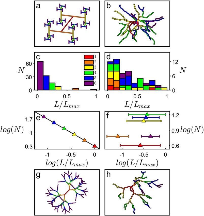
www.nature.com/scientificreports/
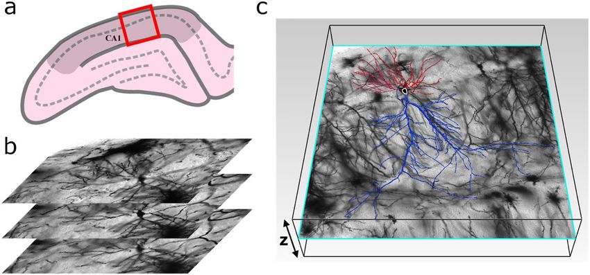
Figure 1. (a) An example confocal micrograph (x–y layer) showing three neighboring dendritic arbors, each
spanning the oriens (SO), pyramidale (SP), radiatum (SR), and lacunosum-moleculare (SLM) strata of the
CA1 region. The dashed lines represent the strata boundaries and the bar corresponds to 100 μm. (b) A three-
dimensional model of a dendritic arbor (reconstructed from a stack of micrographs in the z direction using
(black). The neuron’s axon arbor is not shown. (c) Schematic showing the neuron parameters L, W, ϕ, and θ. (d)
Neurolucida and displayed using MATLAB) featuring the apical (blue) and basal (red) arbors and the soma
Histogram of N, the number of neurons with a given D value, measured for the neurons’ apical and basal arbors.
length, forking, and weaving behavior, we propose that the neuron D values reflect a network cooperation that
optimizes these constraints, with connectivity outweighing cost for neurons with high D values. Remarkably, D
captures this functional optimization even though the fractal-like scaling behavior occurs over a highly limited
range of size scales.
We use confocal microscopy to obtain images of CA1 pyramidal neurons in the coronal plane of the dorsal rat
hippocampus (Figs. 1a, 6). Their somata are located in the stratum pyramidale (SP) of the CA1 region. Axonal
and dendritic arbors extend from each soma, with the dendritic arbor featuring component apical and basal
arbors. The complex branching patterns of these dendritic arbors extend into the neighboring stratum radiatum
(SR) and stratum oriens (SO) of the CA1 region where they collect signals from the axons of other neurons26.
These axons originate either from within the CA1 region and connect to the dendritic arbors from every direc-
tion (e.g. O-LM cells, basket cells, bistratified cells, and axo-axonic cells)37, or they originate from other regions
such as the neighboring CA2 which extends axons parallel to the strata (e.g. Schaffer collaterals). We construct
three-dimensional models of the dendritic arbors (Fig. 1b) from the confocal images of ~100 neurons using
Neurolucida software38 (“Methods”). The branches in the model are composed of a set of cylindrical segments
θ are defined as the angles between connecting segments along the branch. We define the fork angle ϕ as the
which have a median length and width W of 2.4 μm and 1.4 μm, respectively (Fig. 1c). The branch ‘weave’ angles
The distinct median values for θ (12°) and ϕ (37°) motivated our approach of treating ϕ as a separate parameter
first of the branch weave angles (Fig. 1c and “Methods”) for any branch not emanating from the neuron’s soma.
from θ. Associated with each ϕ and θ value, there is an additional angle measuring the segment’s direction of
rotation around the dashed axes in Fig. 1c. The branch length L is defined as the sum of segment lengths between
the forks. As an indicator of arbor size, the maximum branch length Lmax varies between 109–352 μm across all
Scientific Reports | (2021) 11:2332 | https://doi.org/10.1038/s41598-021-81421-2 2
Vol:.(1234567890)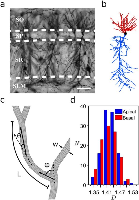
www.nature.com/scientificreports/
neurons, with a median value for L/Lmax of 0.24. Because each parameter (θ, ϕ, and L) features a distribution of
sizes (Fig. 7, Supplementary Fig. 1), we will investigate their potential to generate fractal branch patterns and
consequently their impact on neuron wiring connectivity.
Results
Fractal analysis. In principle, a neuron could extend into the SR and SO layers following a straight line
with dimension D = 1 or spread out and completely fill the space with a dimension of D = 3. If they instead adopt
fractal branches, then these will be quantified by an intermediate D value lying between 1 and 3 1. This fractal
dimension quantifies the relative contributions of coarse and fine scale branch structure to the arbor’s fractal
shape (fractals with larger contributions of fine structure will have higher D values than fractals with lower con-
tributions of fine structure). Whereas a variety of scaling analyses have been applied to neurons14,17,19,22,27,39–43,
here we adopt the traditional ‘box-counting’ technique to directly quantify their D value (“Methods”). This
technique determines the amount of space occupied by the neuron by inserting it into a cube comprised of a
three-dimensional array of boxes and counting the number of boxes, Nbox, occupied by the dendrites (Fig. 8).
This count is repeated for a range of box sizes, Lbox. Fractal scaling follows the power law Nbox ~ Lbox−D. Note that
the box-counting analysis is applied to individual neurons and not to the network of multiple neurons: fractal
networks often ‘space-fill’44 and it is the D values of their fractal elements that determine how they interact11. The
histogram of Fig. 1d plots the number of neurons N with a given D value for both apical and basal arbors. The
medians of their distributions are D = 1.41 (basal) and 1.42 (apical), indicating that their branches have similar
scaling characteristics despite the apical arbors having longer branches that typically feature more forks. Given
that D can assume values up to 3, it is intriguing that the dendrites’ D values are relatively low. Additionally, the
scaling range over which the neurons can be described by this D value is limited to approximately one order of
magnitude of Lbox (“Methods”). This is inevitable because the coarse and fine scale limits are set by the widths of
the arbor and its branches, respectively (“Methods”). We will show that this scaling behavior is so effective that
its limited range is sufficient for the low D values to optimize the connectivity process. Accordingly, D serves as
an ‘effective’ fractal dimension for quantifying neuron functionality despite lacking the range associated with
To clarify this favorable functionality, we first need to determine which parameters (θ, ϕ, and/or L) contrib-
mathematical fractal exponents.
ute to the neuron’s fractal-like character. In mathematics, fractals can be generated by using forking angles (e.g.
Self-contacting Trees, so named because their branch tips intersect), weave angles (e.g. Peano curves), or branch
lengths (e.g. H-Trees)1. Because many mathematical fractals are generated by scaling L, we start by comparing the
neurons’ L behavior to that of H-Trees (“Methods”, Supplementary Fig. 2). Figure 2 shows the scaling relationship
of N (the number of branches with a given L/Lmax) measured for a D = 1.4 H-Tree (Fig. 2a,c,e) and a typical basal
arbor (Fig. 2b,d,f). We assign the branch levels such that i = 1 corresponds to branches emerging from the soma,
i = 2 to the branches emerging from the first forks, etc., with neurons featuring a median of 7 levels on the basal
side and 24 levels on the apical side (other common level assignments such as the Strahler s cheme45 generate
similar findings to those below). The H-Tree exhibits the well-defined reduction in L/Lmax as i increases (Fig. 2c)
and follows the expected power law decrease in N as L/Lmax increases (Fig. 2e): the magnitude of the data line’s
gradient in Fig. 2e equals the H-Tree’s D value of 1.4. This behavior is absent for the neuron: in Fig. 2d, L/Lmax
does not exhibit a systemic reduction in i and consequently the Fig. 2f data does not follow a well-defined slope.
Visual inspection of the equivalent Fig. 2d data for all of the neurons reveals no clear systematic dependence of
their L distributions on D (6 representative neurons are shown in Supplementary Fig. 3). The neurons’ fractal-
like character is even preserved when the L/Lmax distribution is suppressed by setting all branch lengths equal
(for the neuron shown in Fig. 2h, this common length is chosen such that the combined length of all branches
matches that of the undistorted neuron of Fig. 2b). The median D value of the basal arbors drops from 1.41 to
1.30 during this suppression. This occurs because the lower branch levels of the undistorted neuron are consist-
ently shorter than the higher levels45 (Supplementary Fig. 1). This characteristic is removed when the branch
lengths are equated, so pushing the branches further apart and generating the drop in the ratio of fine to coarse
bution, H-Trees with a sufficient number of levels exhibit the expected non-fractal behavior (D = 3) for ϕ = 90°,
structure seen in comparisons of Fig. 2b,h. Significantly, when we similarly suppress their branch length distri-
but display the limited-range fractal behavior if we instead assemble the H-Tree using the neurons’ median ϕ
value (Fig. 2g). This highlights the important role of branch angles coupled with their length distributions for
determining the fractal-like appearance.
This finding opens up an appealing strategy for exploring how the neuron’s D value influences its functionality.
In Fig. 3, we mathematically manipulate the weave angles by multiplying every θ value by a common factor α
(Fig. 7). This changes the neuron’s D value as follows. Values of α higher than 1 increase the weave angles above
their natural values and cause the neuron branches to curl up. We set the highest value to be α = 2 to ensure that
branches rarely intersect and penetrate, so ensuring a physically reasonable condition. As shown by the blue line
in Fig. 3, this curling process causes the D value to rise because the amount of fine structure in the neuron’s shape
increases. Similarly, reducing α causes the branches to gradually straighten out and this reduces the amount of
fine structure and D drops. Figure 3 includes a visual demonstration of this curling process. Interestingly, a key
feature of curling—that total branch length does not rise with D—is also displayed by the undistorted neurons
Applying this technique to ϕ, and also to θ and ϕ simultaneously (Supplementary Fig. 4), we find that either
(and deliberately incorporated into our H-Trees), further emphasizing the appropriateness of this technique.
increasing or decreasing α results in a rise in D. This is because the branches self-avoid at α = 1 and so move
structure. Plots of D directly against the means of θ and ϕ are shown in Supplementary Fig. 5.
closer together when α is either increased or decreased. This generates an increase in the ratio of fine to coarse
Scientific Reports | (2021) 11:2332 | https://doi.org/10.1038/s41598-021-81421-2 3
Vol.:(0123456789)
www.nature.com/scientificreports/
Figure 2. A D = 1.4 H-Tree fractal (generated using Mathematica and displayed using MATLAB) with
W = 1 μm (a) and an example neuron’s basal arbor (reconstructed using Neurolucida and displayed using
MATLAB) with median W = 1.4 μm (b). The branch level i is colored as follows: red (1st branch), orange (2nd),
yellow (3rd), green (4th), blue (5th), and purple (6th). Histograms for an H-Tree (c) and neuron (d) plotting the
number of branches N with a given value of L/Lmax. Panels (e) and (f) show the analysis of (c) and (d) plotted in
lengths to be equal. Additionally, the H-Tree’s forking angle ϕ has been adjusted to 37° (the median value of the
log–log space. Panels (g) and (h) take the H-Tree and neuron shown in (a) and (b) and adjust all their branch
basal arbors).
Connectivity analysis. We now investigate the impact of changing D on the neuron’s potential to connect
to other neurons. Previous studies established that the arbor’s physical structure is sufficient for describing the
connection process, with chemical steering playing a relatively minor role46,47. In particular, the arbor’s dendritic
density33,48–50 and resulting physical profile27 are powerful indicators of its potential to connect to other neu-
rons. When viewed from a particular orientation, we define the arbor’s profile P as the total projected area of
its branches. Large profiles will therefore result in the increased exposure of synapses, which are responsible for
receiving signals from other neurons. When calculating the profile from the dendrite images, we incorporate an
extra layer (orange in Fig. 3 upper inset, Supplementary Fig. 6) surrounding the branches (black) to account for
outgrowth of dendritic spines—small protrusions which contain the majority of the dendrite synapses (“Meth-
ods”). For each arbor shown in Fig. 3, P is therefore the sum of the projected black and orange areas. We then
normalize this projected surface area of the dendrites using their total surface area, As, to accommodate for the
range in neuron sizes and associated surface areas. (Because the orange areas are included in P but not in As, note
Scientific Reports | (2021) 11:2332 | https://doi.org/10.1038/s41598-021-81421-2 4
Vol:.(1234567890)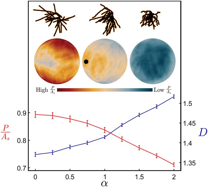
www.nature.com/scientificreports/
Figure 3. P/As (the arbor’s profile, P, averaged over all orientations and normalized to the arbor’s surface area,
As) (red) and fractal dimension D (blue) plotted against the weave angle manipulation factor α for the range
of α resulting in physically reasonable model conditions. The data shown here for both the red and blue lines
are averaged over all basal arbors and their variations are represented by the shown standard errors from the
mean. The upper insets show an example neuron’s basal arbor for α = 0.25 (left), 1 (middle) and 1.75 (right). The
neuron, reconstructed using Neurolucida, was altered and displayed using MATLAB. The lower insets show
the equivalent profile spheres, where the black dot represents the orientation with maximal P/As for the middle
neuron and the bar indicates the colors ranging from high to low P/As values.
that P/As > 1 is possible). The current study adopts the general approach of averaging P/As across all orientations
of the dendritic arbor to allow for the fact that axons originating from within the CA1 region connect to the
dendritic arbors from every direction37. The profile variation with orientation can be visualized by projecting the
P/As values obtained for each direction onto a spherical surface. For the profile spheres included in Fig. 3, the
neurons are viewed from a common direction which corresponds to the middle point on the sphere’s surface. For
the natural neuron, the orientation for which P/As peaks is marked by the black dot. Typically, this peak occurs
in the direction that the Schaffer collateral axons enter from the CA2 r egion26 and so maximizes the connectivity
of our natural neurons to those incoming axons.
The inverse relationship between P/As and D observed when adjusting the weave angle in Fig. 3 also occurs
when adjusting the fork angle (Supplementary Fig. 4). Its physical origin can be traced to the increased fine
structure of high D neurons causing branches to block each other and so reduce the overall profile. Including
this blocking effect is important for capturing the neuron’s connectivity because multiple connections of an axon
to the same dendritic arbor are known to generate redundancies27. Therefore, if a straight axon connected to an
exposed branch, subsequent connections to blocked branches wouldn’t increase the connectivity and should be
their θ and ϕ values manipulated independently. Figure 4b demonstrates that this blocking reduction in P/As is
excluded. Figure 4a summarizes this blocking effect by plotting P/As directly against D for arbors that have had
also seen for H-Trees (which have had their weaves similarly adjusted—see “Methods” and Supplementary Fig. 2),
highlighting that the blocking dependence on D is general to fractals. Figure 4c,d explore another well-known
fractal effect that high D fractals increase the ratio of the object’s surface area As to its bounding area Ab1,2 (i.e.
the surface area of the volume containing the arbor, as quantified by its convex hull—see “Methods”). Figure 4e,f
combines the ‘increased surface area effect’ seen in Fig. 4c,d with the ‘blocking area effect’ seen in Fig. 4a,b by
plotting P/Ab (i.e. the multiplication of P/As and As/Ab) against D. In effect, P/Ab quantifies the large surface area
of the arbor while accounting for the fact that some of this area will be blocked and therefore excluded from the
profile P. Normalizing P using Ab serves the additional purpose of measuring the arbor’s potential connectiv-
ity in a way that is independent of its size. Accordingly, P/Ab serves as a connectivity density and is an effective
measure of the neurons’ capacity to form a network.
The clear rise in P/Ab revealed by Fig. 4e,f highlights the functional advantage offered by high D branches—
incoming axons will experience the dendritic arbor’s large connectivity density. Note that the plotted connectivity
density is for individual neurons. Because of the inter-penetrating character of dendritic arbors from neighboring
neurons, the collective connectivity density will be even larger due to their combined profiles. If this functionality
was the sole driver of neuron morphology, then all neurons would therefore exploit high D values approaching 3.
Yet, both the apical and basal dendrites cluster around relatively low values of D ~ 1.41 suggesting that there are
additional, negative consequences of increasing D. In Fig. 4g,h, we plot the ratio of the volume occupied by the
branches Vm to the neuron’s bounding volume Vb (i.e. the arbor’s convex hull volume). For high D dendrites, the
Scientific Reports | (2021) 11:2332 | https://doi.org/10.1038/s41598-021-81421-2 5
Vol.:(0123456789)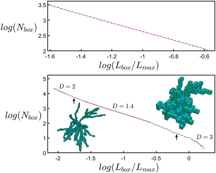
www.nature.com/scientificreports/
Figure 4. Dependences of various parameters (see text for parameter definitions) on D for neurons (left
basal arbors where either their θ or ϕ values are manipulated. H-Trees with straight and with weaving branches
column) and H-Trees (right column). Red data are for unmanipulated basal arbors while the blue data are for
are included. The cyan lines correspond with binned averages of the plots while the black curves correspond to
3rd degree polynomial fits to the data.
tighter weave angles along with forking angles that bring branches closer together result in more densely packed
structures. This produces the observed rise of Vm/Vb. Assuming constant tissue density, Vm is proportional to the
neuronal mass. The rise in Vm/Vb therefore quantifies the increase in mass density and associated ‘building’ costs
of high D neurons. Aside from this, there is also an ‘operational’ cost. It is well-known from allometric scaling
relationships that metabolic costs generally increase with m ass8,10. Specifically, previous research proposed that
the amount of ATP expended by neurons increases with As27,30. Revisiting Fig. 4a,c, As/Ab therefore charts how
the normalized energy cost increases with D, and P/As measures the neuron connectivity relative to this cost. In
Figs. 3 and 4, we didn’t apply the α multiplication technique to the neurons’ distribution of L values because this
would simply change the size of the arbors and have no impact on their fractal characteristics.
Discussion
Taken together, the panels of Fig. 4 summarize the competing consequences of increasing D for both the neurons
and H-Trees: the benefits of enhanced connectivity density increase (Fig. 4e,f), but so does the cost of building
(Fig. 4g,h) and operating (Fig. 4c,d) the branches. The distinct forms of these 3 factors are highlighted using 3rd
degree polynomial fits (black) which closely follow the binned average values of the data (cyan). This observation
of neuron behavior across large D ranges provides a clear picture of their tolerances for the above factors and
highlights both the shared behavior and subtle differences to standard mathematical fractals such as H-Trees. In
particular, the high operating cost, the sharp increase in building cost, and the flatter gradient of the connectiv-
ity curve at high D could explain why the natural neurons (red) don’t exceed D = 1.51. Nor do they occur below
D = 1.33 because of the low connectivity. To explore how the fractals balance these factors, in Fig. 5 we consider
the ratios of the rates of change of connectivity density with operating cost
d P
dD Ab
RPA =
d As
dD Ab
and with building cost
d P
dD Ab
RPV =
d Vm
dD Vb
Scientific Reports | (2021) 11:2332 | https://doi.org/10.1038/s41598-021-81421-2 6
Vol:.(1234567890)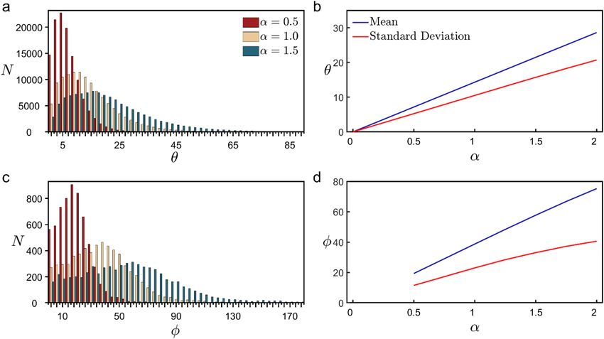
www.nature.com/scientificreports/
Figure 5. The ratio RPA of the derivatives of P/Ab and As/Ab for the neurons (a) and H-Trees (b), along with the
ratio RPV of the derivatives of P/Ab and Vm/Vb for the neurons (c) and H-Trees (d). The blue sections correspond
to the data range shown in Fig. 4, while the green sections correspond to extending the fits to beyond that data
range. The dashed curves in (a) and (c) indicate the effect on RPA and RPV of removing the dendritic spines
from the model. The peaks of the solid curves in (a), (b), (c), and (d) occur at D = 1.26, 1.34, 1.32, and 1.34,
respectively. The peaks of the dashed curves in (a) and (b) occur at D = 1.32 and 1.36, respectively.
as simple optimization indicators. An in-depth comparison of the four curves in Fig. 5 is limited by the fits in
Fig. 4 (in particular, the data scatter and the fact that we can’t increase the D range without resorting to α values
that result in physically unreasonable model conditions, see earlier). Nevertheless, we note the following shared
characteristics: (1) the occurrence of a peak at low D, (2) RPA < 1 (i.e. the connectivity increases more slowly than
the energy costs), and (3) RPV > 1 (the connectivity increases more rapidly than the mass costs). Consequently,
although high D offers superior connectivity for the neurons, the positive consequences of increasing D beyond
the peak rapidly diminish in terms of the mass costs of establishing connectivity. Simultaneously, the negative
consequences of increasing D rapidly rise in terms of the energy costs of establishing connectivity. Figure 5a,c
includes a comparison of our model including and excluding the spine layer to highlight the sensitivity of the
curves to connectivity. As expected, removal of the spines triggers an overall drop in RPA and RPV, and their
peaks shift to higher D values in an attempt to regain connectivity. Intriguingly, the peaks in Fig. 5a,c suggest
an optimized D value lower than the natural neurons’ prevalent D value (for example, RPV peaks at D = 1.32
compared to D = 1.41 in Fig. 1d). Given that the spine layer width is the only input parameter to the model
and its complete exclusion is insufficient to raise the optimization values up to D = 1.41, Fig. 5 suggests that the
optimization process places a greater emphasis on connectivity than our simple ratios would suggest. A previ-
ous study27, which limited its focus to the optimization condition, also under-estimated the neuron scaling
exponent slightly (1.38), although we note that the 2 exponents are not identical—their exponent characterized
small sections of the arbor compared to the overall arbor D presented here. Given that other fractal studies of
neurons employed additional scale-invariance measures such as multifractal dimensions and lacunarity6, our
future studies will expand the approaches of Figs. 4 and 5 to determine if including these measures allows for a
more accurate prediction of the peak values.
Based on our analysis spanning large D ranges beyond their naturally occurring conditions, we hypothesize
that different neuron types have different D values depending on the relative importance of connectivity and
cost. Neurons with a greater need for connectivity will optimize around higher D. For example, human Purkinje
cells are characterized by D ~ 1.818. We also hypothesize that pathological states of neurons, for example those
with Alzheimer’s disease, might affect the fractal optimization and explain previous observations of changes in
the neurons’ scaling b ehavior51. Whereas the above discussions focus on connections to neighboring neurons,
their fractal branching will also optimize connections to neighboring glial cells to maximize transfer of nutrients
and energy. Intriguingly, CA1 hippocampal glial cells have been shown to have similar D values to the neurons
in our study (D = 1.42)52.
Fractal analyses of a wide variety of neurons indicate that their D values don’t generally exceed D = 217,23, pre-
sumably because of the excessive costs of higher D fractals. For comparison, we note that a sphere (D = 3) achieves
Scientific Reports | (2021) 11:2332 | https://doi.org/10.1038/s41598-021-81421-2 7
Vol.:(0123456789)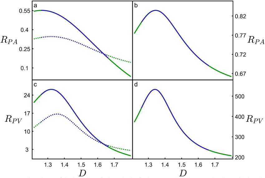
www.nature.com/scientificreports/
much higher connectivity (P/Ab = 0.25 compared to the D = 1.4 neuron’s 0.1). However, the sphere suffers from
large mass density (Vm/Vb = 1 compared to 1 0–3) and higher operational costs (As/Ab = 1 compared to 0.1), sug-
gesting that neurons adopt fractal rather than Euclidean geometry in part because the mass and operational costs
of the latter are too high. We note that neurons’ restriction to lower D values doesn’t apply to fractal electrodes
designed to stimulate neurons53–55. These artificial neurons require large profiles to physically connect to their
natural counterparts. However, unlike natural neurons, the large As associated with high D electrodes reduces
elds53,54. Thus,
the operation costs because their higher electrical capacitances lead to larger stimulating electric fi
fractal electrodes approaching D = 3 might be expected to efficiently connect to and stimulate neurons. That said,
there might be advantages of matching the electrode’s D value to that of the neuron: this will allow the neuron
to maintain its natural weave and forking behavior as it attaches to and grows along the electrode branches, so
maintaining the neuron’s proximity to the stimulating field.
Previous studies of connectivity and dendritic cost focused on component parameters of the neuron geom-
etry such as tortuosity (which quantifies branch weave using, for example, a simple ratio of branch length to the
direct distance between the branch start and end points), branch length, and scaling analysis of small parts of the
arbor27,33. We have shown that our ‘effective’ D incorporates these parameters in a holistic approach that directly
the neurons’ weave (generated by variations in θ and ϕ) is an important factor in determining D provides a link
reflects the fractal-like geometry across multiple branches of the neuron’s arbor. For example, our discovery that
between D and tortuosity. However, whereas tortuosity quantifies the weave of an individual branch measured
at a specific size scale, D captures a more comprehensive picture by accounting for the weave’s tortuosity across
multiples scales. Future studies will examine the precise relationship between D and the scaling properties of
Because D is sensitive to 3 major branch parameters (θ, ϕ, and L), it is a highly appropriate parameter for
tortuosity for both individual branches and the whole arbor.
charting the connectivity versus cost optimization discussed in this Article. Whereas we have focused on this
D-dependent optimization, the future studies will further examine the intricacies of how the branch parameters
D values on θ and ϕ (Supplementary Fig. 5) and a drop in D when their branch lengths are equalized (Fig. 2h).
determine D and T. Here, we have seen that the distorted neurons show systematic dependencies of their mean
We emphasize, however, that the interplay of these 3 dependences generates variations in the individual neu-
D values do not exhibit any clear dependence on θ and ϕ when plotted independently (Supplementary Fig. 5)
rons’ D values and these are responsible for the spread in D observed for the natural neurons (Fig. 1d). Their
and, as noted earlier, the spread in D does not display any systematic dependence on their L distributions. It is
not clear if these D variations between natural neurons are simply obscuring the systematic behavior followed
by the distorted neurons or whether, more intriguingly, the natural neurons are using this interplay of the three
dependences to anchor their D values around the narrow range that results in the optimization condition. The
future investigations aim to illuminate this interplay.
Finally, our focus on D to investigate neurons facilitates direct comparisons with the favorable functionali-
ties generated by diverse structures. Here, we compared our neurons to distorted versions, to H-Trees, to fractal
electrodes, and to Euclidean shapes, but this approach could readily be extended to many natural fractals. The fact
that the H-Trees and neurons exploit a similar D-dependent optimization process (Figs. 4 and 5) raises the ques-
tion of why the two structures use different branch length distributions (Fig. 2) to generate their scaling behavior.
The answer lies in the neuron’s need to minimize signal transport times within the a rbor56. This is achieved with
short branches close to the soma (Supplementary Fig. 1) while the H-Tree suffers from longer branches. Remark-
ably, Figs. 4 and 5 show that the D-dependent behavior impacts neuron functionality even though it occurs over
only a limited range of branch sizes. Many physical fractals are also limited57, demonstrating the effectiveness
of fractal-like behavior for optimizing essential processes ranging from oxygen transfer by our lungs, to light
collection by trees, to neuron connections throughout the body. For neurons, we have shown how they use this
limited fractality to balance wiring connectivity with material, energy, volume, and time (signal) costs.
Methods
Rodents. The study was conducted in accordance with ARRIVE guidelines. Rat pups were bred and housed
with their mother in cages with wood chips and ad libitum food and water in an environmentally controlled
room. All procedures pertaining to the use of live rats were conducted in compliance with all relevant ethical
regulations for animal testing and research and were approved by the University of Canterbury Animal Ethics
Committee, 2008-05R.
Image acquisition and model reconstruction. Thirty-three adult PVGc male hooded rats (13–
16 months old) were given an overdose of sodium pentobarbital. The brains were removed fresh without perfu-
sion, rinsed with Milli-Q water, and a 4 mm block containing the hippocampus was cut in the coronal plane
using a brain matrix (Ted Pella, Kitchener, Canada). These tissue blocks were processed with a metallic Golgi-
Cox stain, which stains 1–5% of neurons so that their cell bodies and dendritic trees can be visualized. Thick
200 µm coronal brain sections spanning the bilateral dorsal hippocampus were taken using a microtome. A
standard microscope was used to locate isolated neurons in the dorsal CA1 subfield (Fig. 6a). These large pyram-
idal neurons consist of a long apical dendritic tree protruding from the apex of the soma and a shorter basal
dendritic tree protruding from the other end (Fig. 1b). Only some intact whole neurons were located, whereas
many intact basal-only or apical-only dendritic trees were located. In total, 105 basal and 113 apical arbors were
imaged. A Leica laser scanning confocal microscope was used to collect high-resolution image stacks for each of
these neuronal processes (Fig. 6b). The image stacks were captured using a 20 × glycerol objective lens with a 0.7
numerical aperture, providing an x and y resolution of 0.4 µm. The step size (z distance between image stacks)
was 2 µm. Dendritic arbors were manually traced through the image stacks using Neurolucida38 (MBF Biosci-
Scientific Reports | (2021) 11:2332 | https://doi.org/10.1038/s41598-021-81421-2 8
Vol:.(1234567890)www.nature.com/scientificreports/
Figure 6. (a) Schematic diagram of a coronal slice through the hippocampus at Bregma −4.52 mm showing
the collection region (red box) within hippocampal CA1 (darkened area); the somata layer is denoted by the
dashed line. (b) Confocal micrographs of Golgi-Cox stained cells. Three 774 by 774 µm cross-sections separated
by 2 µm in the z-direction are shown. (c) A model showing a neuron’s soma (outlined in white) as well as its
basal (red) and apical (blue) dendritic arbors superimposed on the original micrograph. The image in (c) was
generated using Neurolucida.
Figure 7. Histograms of the number N of occurrences of weave (a) and fork (c) angle values across all basal
arbors used in the study. The impact of modifying these angles is shown for three α values. (b,d) Changes to the
peak and breadth of the distribution of these angles as a function of α shown for the range of α that results in
physically reasonable model conditions (see Fig. 3 and Supplementary Fig. 4).
ence, Williston, VT, USA) to create three-dimensional models (Figs. 1b, 6c). The models were then exported to
the Wavefront .obj format and the cell soma removed. The analysis of these models was done by authors of this
study that were blinded to rat ID numbers.
The three-dimensional models are composed of a set of connected hollow cylinders (segments) which form
the branches of the arbors. Each cylinder is constructed using two sets of rings of 16 points (vertices) and 32
connecting triangles (faces). At branch endings, the final segment has 14 faces that form an end cap. Connect-
ing branches start new segments at the same location as the last set of 16 vertices from the previous branch. For
Scientific Reports | (2021) 11:2332 | https://doi.org/10.1038/s41598-021-81421-2 9
Vol.:(0123456789)www.nature.com/scientificreports/
Figure 8. log(Nbox) plotted against log(Lbox/Lmax) for an example neuron’s dendritic arbor, where Nbox is the
number of occupied boxes and Lbox is the box length. The top graph shows a zoom-in on the fractal-like scaling
region of the bottom graph. The insets show occupied boxes at small and large box scales. See the text for
explanations of the arrows.
the apical arbors, one branch extends from the apex of the soma and all other branches connect either directly
or indirectly to it. For the basal arbors, multiple initial branches extend from the soma, each with its own set of
connecting branches.
In order to perform the box-counting and profile analyses, the Wavefront files were converted to voxel data
using custom MATLAB code. The voxelization was performed at a resolution of 4 voxels/µm for box counting
and 1 voxel/µm for the profile calculation. In both cases, the models were voxelized “exactly,” meaning that if any
part of the polygonal model fell inside a voxel, the voxel was added to the list of x; y; z coordinates.
We used rotation quaternions58 to adjust the weave and fork angles to the modified values multiplied by the
pre-factor α When adjusting the weave angles, we started with the angles furthest from the soma and, work-
ing inwards, adjusted angles one at a time until all of the angles had acquired their new values. When an angle
was adjusted, the entire connected section of the branch between that angle and the terminal endcaps was also
rotated. This rotation occurred in the plane of the two vectors that define that angle. We created three sets of
modified, in a second set ϕ was modified, and in a third set both were modified simultaneously. The effect that
arbor models modified by the multiplier α for values between 0 and 2, incremented by 0.25. In one set θ was
the multiplier α has on the distribution of weave and fork angles can be seen in Fig. 7. Because our investigation
focused on weaving and forking deviations relative to the dashed lines shown in Fig. 1c, their measured angles
do not distinguish between whether the branches fall to the left or right of these lines. Accordingly, for the rare
examples when the α multiplication generated angles greater than 180° (corresponding to branches crossing
over the dashed line) the angles were adjusted so that they remain within the range between 0° and 180°. For
example, when α = 2 was applied to a natural forking angle of 100°, the resulting angle was measured as 160°
rather than 200°. This measurement scheme caused the slight non-linearity seen at large α values for the red and
blue curves of Fig. 7d. The percentages of weave angles crossing the dashed line were 0.009% and 0.07% when
α = 1.5 and 2, respectively. The corresponding percentages for the forking angles were 0.7% and 2.7%. We note
that the measurement scheme did not impact the conclusions of this Article. For completeness, we also note that
if we did not distinguish between the forking and weave angles and instead treated them as one set of angles,
the combined distribution of angles would follow a similar behavior to that shown in Fig. 7a,b because of the
relatively small number of forking angles.
When calculating the surface area, As, of the models, the precision was raised by increasing the number of
faces in a neuron’s construction four-fold by converting each triangle into four sub-triangles using a midpoint
method (Supplementary Fig. 7). We then summed the areas of all the triangles in the model, excluding the faces
where all three vertices resided inside another segment. The bounding area, Ab, and bounding volume, Vb, were
calculated using the convex hull m ethod59 on the vertices of the Wavefront object. Ab is the sum of the areas
of all triangles composing the convex hull that encloses the vertices, whereas Vb is the volume enclosed within
those triangles.
Box counting analysis. The box-counting method used to analyze the fractal characteristics of the neu-
rons is shown in Fig. 8. Using custom MATLAB code, the voxelized dentritic arbor was inserted into the three-
dimensional array of boxes and the number of boxes Nbox occupied by the neuron were counted for different sizes
of boxes, Lbox, and this was normalized to Lmax, the largest branch size of the arbor. The largest box size was set to
the size of the longest side length of the arbor’s bounding box and the smallest box size to the voxel pixelization
Scientific Reports | (2021) 11:2332 | https://doi.org/10.1038/s41598-021-81421-2 10
Vol:.(1234567890)www.nature.com/scientificreports/
(0.25 µm). The insets show example schematics of the filled boxes for large and small Lbox values. We performed
a modified ‘sliding’ box count13 in which the boxes slid in every coordinate direction simultaneously in 0.25 µm
steps and the minimum count was selected.
Fractal scaling, Nbox ~ Lbox-D, appears as a straight line in the log–log plot. The range of Lbox/Lmax values for
which fractal behavior might be observed lies between the vertical arrows. For large boxes to the right of the right
arrow, there are too few boxes (less than five along each side of the bounding box) to reveal the fractal behavior.
Consequently, all of the boxes become filled and so the analysis interprets the neuron as being three-dimensional
and the gradient eventually shifts to a value of three. To the left of the left arrow (corresponding to 2 μm), the box
sizes approach the diameters of the branches and so the analysis starts to pick up the two-dimensional character
of the branches’ surface and the gradient shifts to a value of two.
Between the arrows, a straight line was fitted for all sets of points ranging over at least one order of magnitude.
The fit that maximized R2 was chosen to measure the D value (the slope of the line). When looking at the residu-
als of this regression analysis, their behavior confirmed that the fit range was appropriate. We note that applying
the angle multiplier to the neurons didn’t reduce the quality of the fit nor the scaling range of fractal behavior.
Profile analysis. An arbor’s physical p rofile27 has been shown to be intrinsically related to its ability to
connect with other neurons. We developed custom MATLAB code that measures the profile of the dendritic
arbor using a list of cartesian points in space that denote the locations occupied by the dendrites. In our calcu-
lations, we used the voxelized list of points generated using the Wavefront file of the dendritic arbor. To allow
the dendritic spines to contribute to the calculation of an arbor’s profile, we uniformly expanded the voxelized
arbor by 2 µm in every direction. The orange region around the black dendrites seen in Supplementary Fig. 6
represents the space around the dendrites in which a spine could grow in order to form a synapse with an axon
passing through the arbor. Including a solid orange region assumes a high spine density. Lower densities could
be accommodated by reducing the profile by a density pre-factor. Given the comparisons in the current study
are made across the same neuron type with the same spine density, the value of the pre-factor will not impact
the results.
This expanded list of points was then orthographically projected onto the x–y plane. After projection, the
points were rounded and any duplicate points occupying the same location were removed. Because the location of
the points has been rounded, each point represents a 1 µm2 area and the total area occupied by this projection can
be measured by counting the number of remaining points constituting the projection. The area of this projection
divided by the bounding area of the neuron is then proportional to the probability of connection with an axon
travelling parallel to the z-direction and passing through the dendritic arbor. However, because the axons that
pass through the arbors of our CA1 neurons can arrive from any d irection26,37, we calculated the average profile
of each neuron’s arbor as though it were viewed from any point on the surface of a sphere containing the neuron’s
arbor with its origin at the neuron’s center of mass. To accomplish this, we defined a set of polar and azimuthal
angles that corresponded to uniformly distributed viewpoints on the sphere. By rotating the expanded list of
points by these angles and then projecting the result onto the x–y plane, we obtained what the arbor would look
like if seen from the given viewpoint. We calculated the average profile by averaging the area of the projections
corresponding with each of our uniformly distributed viewpoints. Because it is impossible to distribute a general
number of equidistant points on the surface of a s phere60, we defined our set of points using the Fibonacci lattice,
a commonly used and computationally efficient method for distributing the points61.
The colored spheres (comprised of 10,001 points) in Fig. 3 and Supplementary Fig. 6 give a visual representa-
tion of the variation in profile with respect to the viewpoint. The average profile data used in Fig. 4 was calculated
using only 201 viewpoints, which is sufficient for convergence—the average P for 201 viewpoints deviates by less
than 1% from the value achieved when approaching infinite viewpoints.
H‑Tree generation. We compare the neurons to H-Trees to identify the similarities and differences to a tra-
ditional mathematical fractal pattern in which D is set by scaling the branch length L (we caution that any simi-
larities do not imply a shared growth m echanism44). Supplementary Fig. 2 shows examples of the H-Tree models
used to generate the data of Fig. 4b,d,f. Whereas these H-Trees extend into three-dimensional space (middle and
bottom row), we also include two-dimensional H-Trees (top row) for visual comparison. Using Mathematica
software, the D values of these straight branched models were generated using the branch scaling relationship
L1
Li = i−1 ,
2 D
where Li is the branch length of the ith level. The H-Trees used to generate the data seen in Fig. 4 had 12 levels
of branches and the length of the first branch, L1, of any given H-Tree was chosen such that the total length of all
the branches was constant across all D values. For comparison of the H-Trees with the basal arbors in Fig. 4, the
number of branch levels in the H-Tree was chosen to be close to the largest number of levels observed for the
basal arbors (11) and the width of the H-Trees branches was chosen to be 1 μm which is similar to the 1.4 μm
median width of the branches for the basal arbors. The D values of H-Trees in the bottom row of Supplementary
Fig. 2 are determined by a combination of the length scaling between branch levels and the weave of the branches.
The distribution of weave angles was generated using a fractional gaussian noise process, which is known to be
self-similar, and the resulting D values were measured using the box-counting algorithm. The width of the weave
angle distribution was specified before generating the H-Tree, allowing for fine control over the tortuosity of
its branches. By using four different weave angle distribution widths and creating H-Trees with a multitude of
D values, we demonstrated the robustness of the relationship between the D value and our various functional
parameters shown in Fig. 4.
Scientific Reports | (2021) 11:2332 | https://doi.org/10.1038/s41598-021-81421-2 11
Vol.:(0123456789)www.nature.com/scientificreports/
Data availability
All data necessary to reproduce the results are available at https: //github
.com/jsmith
767/Neuron
Fract alGeo
metry .
Code availability
All scripts necessary to reproduce the results are available at https://github.com/jsmith767/NeuronFractalGe
ometry.
Received: 18 September 2020; Accepted: 30 December 2020
References
1. Mandelbrot, B. & Pignoni, R. The Fractal Geometry of Nature. 173, (WH freeman, 1983).
2. Bassingthwaighte, J. B., Liebovitch, L. S. & West, B. J. Fractal Physiology. (Springer, New York, 1994).
3. Iannaccone, P. M. & Khokha, M. Fractal Geometry in Biological Systems: An Analytical Approach. (CRC Press, Boca Raton, 1996).
4. West, G. B., Brown, J. H. & Enquist, B. J. The fourth dimension of life: Fractal geometry and allometric scaling of organisms. Science
284, 1677–1679 (1999).
5. Lennon, F. E. et al. Lung cancer-a fractal viewpoint. Nat. Rev. Clin. Oncol. 12, 664–675 (2015).
6. Sapoval, B., Baldassarri, A. & Gabrielli, A. Self-stabilized fractality of seacoasts through damped erosion. Phys. Rev. Lett. 93, 098501
(2004).
7. Li, J. et al. A new estimation model of the lightning shielding performance of transmission lines using a fractal approach. IEEE
Trans. Dielectr. Electr. Insul. 18, 1712–1723 (2011).
8. Banavar, J. R., Maritan, A. & Rinaldo, A. Size and form in efficient transportation networks. Nature 399, 130–132 (1999).
9. Eloy, C. Leonardo’s rule, self-similarity, and wind-induced stresses in trees. Phys. Rev. Lett. 107, 258101 (2011).
10. West, G. B., Brown, J. H. & Enquist, B. J. A general model for the origin of allometric scaling laws in biology. Science 276, 122–126
(1997).
11. Schröter, M., Paulsen, O. & Bullmore, E. T. Micro-connectomics: Probing the organization of neuronal networks at the cellular
scale. Nat. Rev. Neurosci. 18, 131–146 (2017).
12. The Petilla Interneuron Nomenclature Group (PING) et al. Petilla terminology: Nomenclature of features of GABAergic interneu-
rons of the cerebral cortex. Nat. Rev. Neurosci. 9, 557–568 (2008).
13. Smith, T. G. Jr., Lange, G. D. & Marks, W. B. Fractal methods and results in cellular morphology—dimensions, lacunarity and
multifractals. J. Neurosci. Methods 69, 123–136 (1996).
14. Alves, S. G., Martins, M. L., Fernandes, P. A. & Pittella, J. E. H. Fractal patterns for dendrites and axon terminals. Phys. Stat. Mech.
Appl. 232, 51–60 (1996).
15. Wearne, S. L. et al. New techniques for imaging, digitization and analysis of three-dimensional neural morphology on multiple
scales. Neuroscience 136, 661–680 (2005).
16. Zietsch, B. & Elston, E. Fractal analysis of pyramidal cells in the visual cortex of the galago (Otolemur garnetti): Regional variation
in dendritic branching patterns between visual areas. Fractals 13, 83–90 (2005).
17. Caserta, F. et al. Determination of fractal dimension of physiologically characterized neurons in two and three dimensions. J.
Neurosci. Methods 56, 133–144 (1995).
18. Takeda, T., Ishikawa, A., Ohtomo, K., Kobayashi, Y. & Matsuoka, T. Fractal dimension of dendritic tree of cerebellar Purkinje cell
during onto- and phylogenetic development. Neurosci. Res. 13, 19–31 (1992).
19. Milošević, N. T. & Ristanović, D. Fractality of dendritic arborization of spinal cord neurons. Neurosci. Lett. 396, 172–176 (2006).
20. Werner, G. Fractals in the nervous system: Conceptual implications for theoretical neuroscience. Front. Physiol. 1, 15 (2010).
21. Di Ieva, A., Grizzi, F., Jelinek, H., Pellionisz, A. J. & Losa, G. A. Fractals in the neurosciences, Part I: General principles and basic
neurosciences. Neuroscientist 20, 403–417 (2014).
22. Isaeva, V. V., Pushchina, E. V. & Karetin, Yu. A. The quasi-fractal structure of fish brain neurons. Russ. J. Mar. Biol. 30, 127–134
(2004).
23. Kim, J. et al. Altered branching patterns of Purkinje cells in mouse model for cortical development disorder. Sci. Rep. 1, 122 (2011).
24. Ferrari, G. et al. Corneal confocal microscopy reveals trigeminal small sensory fiber neuropathy in amyotrophic lateral sclerosis.
Front. Aging Neurosci. 6, 278 (2014).
25. Morigiwa, K., Tauchi, M. & Fukuda, Y. Fractal analysis of ganglion cell dendritic branching patterns of the rat and cat retinae.
Neurosci. Res. Suppl. 10, S131–S139 (1989).
26. Andersen, P., Morris, R., Amaral, D., Bliss, T. & O’Keefe, J. The Hippocampus Book. (Oxford University Press, Oxford, 2006).
27. Wen, Q., Stepanyants, A., Elston, G. N., Grosberg, A. Y. & Chklovskii, D. B. Maximization of the connectivity repertoire as a
statistical principle governing the shapes of dendritic arbors. Proc. Natl. Acad. Sci. 106, 12536–12541 (2009).
28. Chen, B. L., Hall, D. H. & Chklovskii, D. B. Wiring optimization can relate neuronal structure and function. Proc. Natl. Acad. Sci.
103, 4723–4728 (2006).
29. Laughlin, S. B., de Ruyter van Steveninck, R. R. & Anderson, J. C. The metabolic cost of neural information. Nat. Neurosci. 1, 36–41
(1998).
30. Attwell, D. & Laughlin, S. B. An energy budget for signaling in the grey matter of the brain. J. Cereb. Blood Flow Metab. Off. J. Int.
Soc. Cereb. Blood Flow Metab. 21, 1133–1145 (2001).
31. Mitchison, G. & Barlow, H. B. Neuronal branching patterns and the economy of cortical wiring. Proc. R. Soc. Lond. B Biol. Sci.
245, 151–158 (1991).
32. Cherniak, C. Local optimization of neuron arbors. Biol. Cybern. 66, 503–510 (1992).
33. Chklovskii, D. B. Synaptic connectivity and neuronal morphology: Two sides of the same coin. Neuron 43, 609–617 (2004).
34. Rushton, W. A. H. A theory of the effects of fibre size in medullated nerve. J. Physiol. 115, 101–122 (1951).
35. Rall, W. et al. Matching dendritic neuron models to experimental data. Physiol. Rev. 72, S159–S186 (1992).
36. Wen, Q. & Chklovskii, D. B. Segregation of the brain into gray and white matter: A design minimizing conduction delays. PLoS
Comput. Biol. 1, e78 (2005).
37. Wheeler, D. W. et al. Hippocampome.org: A knowledge base of neuron types in the rodent hippocampus. eLife 4, e09960 (2015).
38. Neurolucida | Neuron Tracing Software | MBF Bioscience. Available at: https://www.mbfbioscience.com/neurolucida. Accessed
26 July 2019
39. Fernández, E., Bolea, J. A., Ortega, G. & Louis, E. Are neurons multifractals?. J. Neurosci. Methods 89, 151–157 (1999).
40. Cuntz, H., Mathy, A. & Häusser, M. A scaling law derived from optimal dendritic wiring. Proc. Natl. Acad. Sci. U. S. A. 109,
11014–11018 (2012).
41. Smith, T. G., Marks, W. B., Lange, G. D., Sheriff, W. H. & Neale, E. A. A fractal analysis of cell images. J. Neurosci. Methods 27,
173–180 (1989).
Scientific Reports | (2021) 11:2332 | https://doi.org/10.1038/s41598-021-81421-2 12
Vol:.(1234567890)You can also read