Vertical dependence of horizontal variation of cloud microphysics: observations from the ACE-ENA field campaign and implications for warm-rain ...
←
→
Page content transcription
If your browser does not render page correctly, please read the page content below
Atmos. Chem. Phys., 21, 3103–3121, 2021
https://doi.org/10.5194/acp-21-3103-2021
© Author(s) 2021. This work is distributed under
the Creative Commons Attribution 4.0 License.

Vertical dependence of horizontal variation of cloud microphysics:
observations from the ACE-ENA field campaign and implications
for warm-rain simulation in climate models
Zhibo Zhang1,2 , Qianqian Song1,2 , David B. Mechem3 , Vincent E. Larson4 , Jian Wang5 , Yangang Liu6 ,
Mikael K. Witte7,8 , Xiquan Dong9 , and Peng Wu9,10
1 Department    of Physics, University of Maryland Baltimore County (UMBC), Baltimore, 21250, USA
2 Joint Center for Earth Systems Technology, UMBC, Baltimore, 21250, USA
3 Department of Geography and Atmospheric Science, University of Kansas, Lawrence, 66045, USA
4 Department of Mathematical Sciences, University of Wisconsin – Milwaukee, Milwaukee, 53201, USA
5 Center for Aerosol Science and Engineering, Department of Energy, Environmental and Chemical Engineering,

Washington University in St. Louis, St. Louis, 63130, USA
6 Environmental and Climate Science Department, Brookhaven National Laboratory, Upton, 11973, USA
7 Joint Institute for Regional Earth System Science and Engineering,

University of California Los Angeles, Los Angeles, 90095, USA
8 Jet Propulsion Laboratory, California Institute of Technology, Pasadena, 91011, USA
9 Department of Hydrology and Atmospheric Sciences, University of Arizona, Tucson, 85721, USA
10 Pacific Northwest National Laboratory, Richland, WA 99354, USA

Correspondence: Zhibo Zhang (zhibo.zhang@umbc.edu)

Received: 29 July 2020 – Discussion started: 11 August 2020
Revised: 3 January 2021 – Accepted: 5 January 2021 – Published: 2 March 2021

Abstract. In the current global climate models (GCMs), the          top. Although this study is based on limited cases, it suggests
nonlinearity effect of subgrid cloud variations on the parame-      that the subgrid variations of Nc and its correlation with qc
terization of warm-rain process, e.g., the autoconversion rate,     both need to be considered for an accurate simulation of the
is often treated by multiplying the resolved-scale warm-rain        autoconversion process in GCMs.
process rates by a so-called enhancement factor (EF). In this
study, we investigate the subgrid-scale horizontal variations
and covariation of cloud water content (qc ) and cloud droplet
number concentration (Nc ) in marine boundary layer (MBL)
clouds based on the in situ measurements from a recent field        1   Introduction
campaign and study the implications for the autoconversion
rate EF in GCMs. Based on a few carefully selected cases            Marine boundary layer (MBL) clouds cover about one-fifth
from the field campaign, we found that in contrast to the           of Earth’s surface and play an important role in the climate
enhancing effect of qc and Nc variations that tends to make         system (Wood, 2012). A faithful simulation of MBL clouds
EF > 1, the strong positive correlation between qc and Nc re-       in the global climate model (GCM) is critical for the projec-
sults in a suppressing effect that tends to make EF < 1. This       tion of future climate (Bony and Dufresne, 2005; Bony et al.,
effect is especially strong at cloud top, where the qc and Nc       2015; Boucher et al., 2013) and understanding of aerosol–
correlation can be as high as 0.95. We also found that the          cloud interactions (Carslaw et al., 2013; Lohmann and Fe-
physically complete EF that accounts for the covariation of         ichter, 2005). Unfortunately, this turns out to be an extremely
qc and Nc is significantly smaller than its counterpart that ac-    challenging task. Among others, an important reason is that
counts only for the subgrid variation of qc , especially at cloud   many physical processes in MBL clouds occur on spatial

Published by Copernicus Publications on behalf of the European Geosciences Union.
3104                                     Z. Zhang et al.: Vertical dependence of horizontal variation of cloud microphysics

scales that are much smaller than the typical resolution of         Given subgrid-scale variability represented as a distribution
GCMs.                                                               P (x) of some variable x, for example the qc inREq. (1), a grid-
   Of particular interest in this study is the warm-rain pro-       mean process rate is calculated as hf (x)i = f (x)P (x)dx
cesses that play an important role in regulating the lifetime,      , where f (x) is the formula for the local process rate. For
water budget, and therefore integrated radiative effects of         nonlinear process rates such as autoconversion and accretion,
MBL clouds. In the bulk cloud microphysics schemes that             the grid-mean process rates calculated from the subgrid-scale
are widely used in GCMs (Morrison and Gettelman, 2008),             variability do not equal the process rate calculated from the
continuous cloud particle spectrum is often divided into two        grid-mean value of x, i.e., hf (x)i 6 = f (hxi). Therefore, cal-
modes. Droplets smaller than the separation size r ∗ are clas-      culating autoconversion and accretion from grid-mean quan-
sified into the cloud mode, which is described by two mo-           tities introduces biases arising from subgrid-scale variability.
ments of droplet size distribution (DSD), the droplet number        To take this effect into account, a parameter E is often in-
concentration Nc (0th moment of DSD), and droplet liquid            troduced as part of the parameterization such that hf (x)i =
water content qc (proportional to the third moment). Droplets       E · f (hxi). Following the convention of previous studies, E
larger than r ∗ are classified into a precipitation mode (drizzle   is referred to as the enhancement factor (EF) here. Given the
or rain), with properties denoted by drop concentration and         autoconversion parameterization scheme, the magnitude of
water content (Nr and qr ). In a bulk microphysics scheme,          EF is primarily determined by cloud horizontal variability
the transfer of mass from the cloud to rain modes as a result       within a GCM grid. Unfortunately, because most GCMs do
of the collision–coalescence process is separated    into
                                                            two    not resolve subgrid cloud variation, the value of EF is often
terms, autoconversion and accretion: ∂q       r
                                            ∂t coal =  ∂qr
                                                       ∂t auto +
                                                                    simply assumed to be a constant for the lack of better options.
                                                                  In the previous generation of GCMs, the EF for the KK auto-
  ∂qr
   ∂t acc . Autoconversion is defined as the rate of mass trans-    conversion scheme due to subgrid qc variation is often simply
fer from the cloud to rain mode due to the coalescence of two       assumed to be a constant. For example, in the widely used
cloud droplets with r < r ∗ . Accretion is defined as the rate      Community Atmosphere Model (CAM) version 5 (CAM5)
of mass transfer due to the coalescence of a rain drop with         the EF for autoconversion is assumed to be 3.2 (Morrison
r > r ∗ with a cloud droplet. A number of autoconversion and        and Gettelman, 2008).
accretion parameterizations have been developed, formulated             A number of studies have been carried out to better un-
either through numerical fitting of droplet spectra obtained        derstand the horizontal variations of cloud microphysics in
from bin microphysics LES or parcel model (Khairoutdinov            MBL cloud and the implications for warm-rain simulations
and Kogan, 2000), or through an analytical simplification of        in GCMs. Most of these studies have been focused on the
the collection kernel to arrive at expressions that link auto-      subgrid variation of qc . Morrison and Gettelman (2008) and
conversion and accretion with the bulk microphysical vari-          several later studies (Boutle et al., 2014; Hill et al., 2015;
ables (Liu and Daum, 2004). For example, a widely used              Lebsock et al., 2013; Zhang et al., 2019) showed that the sub-
scheme developed by Khairoutdinov and Kogan (2000) (“KK             grid variability qc and thereby the EF are dependent on cloud
scheme” hereafter) relates the autoconversion with Nc and qc        regime and cloud fraction (fc ). They are generally smaller
as follows:                                                         over the closed-cell stratocumulus regime with higher fc and

  ∂qr

                                     β
                                                                    larger over the open-cell cumulus regime that often has a rel-
                                          β
             = fauto (qc , Nc ) = Cqc q Nc N ,                (1)   atively small fc . The subgrid variance of qc is also depen-
   ∂t auto
                                                                    dent on the horizontal scale (L) of a GCM grid. Based on
where qc and Nc have units of kg kg−1 and cm−3 , respec-            the combination of in situ and satellite observations, Boutle
tively; the parameter C = 1350 and the two exponents βq =           et al. (2014) found that the subgrid qc variance first in-
2.47 and βN = −1.79 are obtained through a nonlinear re-            creases quickly with L when L is below about 20 km, then
gression between the variables qc and Nc and the autocon-           increases slowly and seems to approach to an asymptotic
version rate derived from large-eddy simulation (LES) with          value for larger L. Similar spatial dependence is also re-
bin-microphysics spectra.                                           ported in Huang et al. (2014), Huang and Liu (2014), Xie
   Having a highly accurate microphysical parameterization          and Zhang (2015), and Wu et al. (2018), which are based on
– specifically, highly accurate local microphysical process         the ground radar retrievals from the Department of Energy
rates – is not sufficient for an accurate simulation of warm-       (DOE) Atmospheric Radiation Measurement (ARM) sites.
rain processes in GCMs. Clouds can have significant struc-          The cloud-regime and horizontal-scale dependences have in-
tures and variations at the spatial scale much smaller than the     spired a few studies to parameterize the subgrid qc variance
typical grid size of GCMs (10–100 km) (Barker et al., 1996;         as a function of either fc or L or a combination of the two
e.g., Cahalan and Joseph, 1989; Lebsock et al., 2013; Wood          (e.g., Ahlgrimm and Forbes, 2016; Boutle et al., 2014; Hill
and Hartmann, 2006; Zhang et al., 2019). Therefore, GCMs            et al., 2015; Xie and Zhang, 2015; Zhang et al., 2019). In-
need to account for these subgrid-scale variations in order to      spired by these studies, several latest-generation GCMs have
correctly calculate grid-mean autoconversion and accretion          adopted the cloud-regime-dependent and scale-aware param-
rates. Pincus and Klein (2000) nicely illustrate this dilemma.

Atmos. Chem. Phys., 21, 3103–3121, 2021                                               https://doi.org/10.5194/acp-21-3103-2021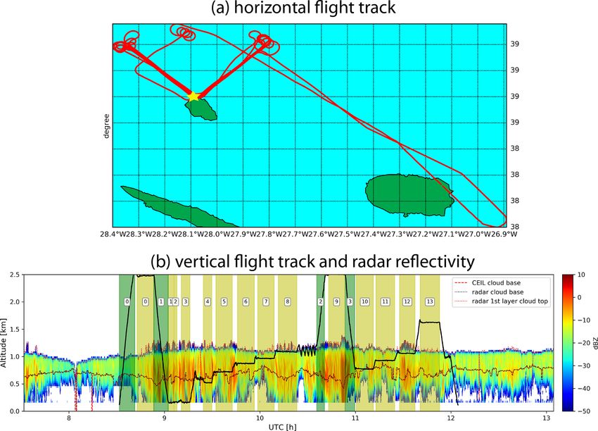
Z. Zhang et al.: Vertical dependence of horizontal variation of cloud microphysics                                           3105

eterization schemes to account for the subgrid variability of      inside the MBL clouds. It is important to understand this de-
qc and thereby the EF (Walters et al., 2019).                      pendence for several reasons. First, the warm-rain process is
   However, the aforementioned studies have an important           usually initialized at cloud top where the autoconversion pro-
limitation. They consider only the impacts of subgrid qc vari-     cess of the cloud droplets gives birth to embryo drizzle drops.
ations on the EF but ignore the impacts of subgrid variation       The accretion process is, on the other hand, more important
of Nc and its covariation with qc . Based on cloud fields from     in the lower part of the cloud (Wood, 2005b). Thus, a better
large-eddy simulation, Larson and Griffin (2013) and later         understanding of the vertical dependence of horizontal vari-
Kogan and Mechem (2014, 2016) elucidated that it is im-            ations of qc and Nc inside MBL clouds could help us under-
portant to consider the covariation of qc and Nc to derive         stand how the EF should be modeled in the GCMs for both
a physically complete and accurate EF for the autoconver-          autoconversion and accretion. Second, a good understanding
sion parameterization. Lately, on the basis of MBL cloud ob-       of the vertical dependence of qc and Nc variation inside MBL
servations from the Moderate Resolution Imaging Spectrora-         clouds will also help us understand the limitations in the pre-
diometer (MODIS), Zhang et al. (2019) (hereafter referred to       vious studies, such as Z19, that use the column-integrated
as Z19) have elucidated that the subgrid variation of Nc tends     products for the study of EF. Finally, this investigation may
to further increase the EF for the autoconversion process in       also be useful for modeling other processes, such as aerosol–
addition to the EF due to qc variation. The effect of qc –Nc       cloud interactions, in the GCMs.
covariation on the other hand depends on the sign of the qc –         Therefore, our main objectives in this study are to (1) bet-
Nc correlation. A positive qc –Nc correlation would lead to an     ter understand the horizontal variations of qc and Nc , their
EF < 1 that partly offsets the effects of qc and Nc variations.    covariation, and the dependence on vertical height in MBL
Although Z19 shed important new light on the EF problem            clouds; and (2) elucidate the implications for the EF of the
for the warm-rain process, their study also suffers from lim-      autoconversion parameterization in GCMs. The rest of the
itations due to the use of satellite remote sensing data. First,   paper is organized as follows: we will describe the data and
as a passive remote sensing technique, the MODIS cloud             observations used in this study in Sect. 2 and explain how we
product can only retrieve the column-integrated cloud optical      select the cases from the ACE-ENA campaign for our study
thickness and the cloud droplet effective radius at cloud top,     in Sect. 3. We will present case studies in Sects. 4 and 5.
from which the column-integrated cloud liquid water path           Finally, the results and findings from this study will be sum-
(LWP) is estimated. As a result of using LWP, instead verti-       marized and discussed in Sect. 6.
cally resolved observations the vertical dependence of the qc
and Nc horizontal variabilities are ignored in Z19. Second,
the Nc retrieval from MODIS is based on several important          2   Data and observations
assumptions, which can lead to large uncertainties (see re-
view by Grosvenor et al., 2018). Furthermore, the MODIS            The data and observations used for this study are from two
cloud retrieval product is known to suffer from several in-        main sources: the in situ measurements from the ACE-ENA
herent uncertainties, such as the three-dimensional radiative      campaign and the ground-based observations from the ARM
effects(e.g., Zhang and Platnick, 2011; Zhang et al., 2012,        ENA site. The ENA region is characterized by persistent sub-
2016), which in turn can lead to large uncertainties in the        tropical MBL clouds that are influenced by different sea-
estimated EF.                                                      sonal meteorological conditions and a variety of aerosol
   This study is a follow-up of Z19. To overcome the limi-         sources (Wood et al., 2015). A modeling study by Carslaw
tations of satellite observations, we use the in situ measure-     et al. (2013) found the ENA to be one of the regions over the
ments of MBL cloud from a recent DOE field campaign, the           globe with the largest uncertainty of aerosol indirect effect.
Aerosol and Cloud Experiments in the Eastern North Atlantic        As such, the ENA region attracted substantial attention over
(ACE-ENA), to investigate the subgrid variations of qc and         the past few decades for aerosol–cloud interaction studies.
Nc , as well as their covariation, and the implications for the    From April 2009 to December 2010 the DOE ARM program
simulation of autoconversion simulation in GCMs. A main            deployed its ARM Mobile Facility (AMF) to Graciosa Is-
focus of this investigation is to understand the vertical de-      land (39.09◦ N, 28.03◦ W) for a measurement field campaign
pendence of the qc and Nc horizontal variations within the         targeting the properties of cloud, aerosol, and precipitation in
MBL clouds. This aspect has been neglected in Z19 as well          the MBL (CAP-MBL) in the Azores region of ENA (Wood et
as most previous studies (Boutle et al., 2014; Lebsock et al.,     al., 2015). The measurements from the CAP-MBL campaign
2013; Xie and Zhang, 2015). A variety of microphysical pro-        have proved highly useful for a variety of purposes, from un-
cesses, such as adiabatic growth, collision–coalescence, and       derstanding the seasonal variability of clouds and aerosols
entrainment mixing, can influence the vertical structure of        in the MBL of the ENA region (Dong et al., 2014; Rémil-
MBL clouds. At the same time, these processes also vary hor-       lard et al., 2012) to improving cloud parameterizations in the
izontally at the subgrid scale of GCMs. As a result, the hor-      GCMs (Zheng et al., 2016) to validating the spaceborne re-
izontal variations of qc and Nc , as well as their covariation,    mote sensing products of MBL clouds (Zhang et al., 2017).
and therefore the EFs may depend on the vertical location          The success of the CAP-MBL revealed that the ENA has an

https://doi.org/10.5194/acp-21-3103-2021                                            Atmos. Chem. Phys., 21, 3103–3121, 2021
3106                                    Z. Zhang et al.: Vertical dependence of horizontal variation of cloud microphysics

ideal mix of conditions to study the interactions of aerosols     Table 1. In situ cloud instruments from ACE-ENA campaign used
and MBL clouds. In 2013 a permanent measurement site was          in this study.
established by the ARM program on Graciosa Island and is
typically referred to as the ENA site (Voyles and Mather,             Instruments   Measurements          Frequency   Resolution   Size
                                                                                                                                   resolution
2013).
                                                                      AIMMS         P , T , RH, u, v, w   20 Hz       –            –
2.1    In situ measurements from the ACE-ENA                          FCDP          DSD 2–50 µm           10 Hz       1–2 µm       2 µm
                                                                      2DS           DSD 10–2500 µm        1 Hz        25–150 µm    10 µm
       campaign

The Aerosol and Cloud Experiments in ENA (ACE-ENA)
project was “motivated by the need for comprehensive in           2.2      Ground observations from the ARM ENA site
situ characterizations of boundary-layer structure and associ-
ated vertical distributions and horizontal variabilities of low   In addition to the in situ measurements, ground measure-
clouds and aerosol over the Azores” (Wang et al., 2016). The      ments from the ARM ENA site are also used to provide ancil-
ARM Aerial Facility (AAF) Gulfstream-1 (G-1) aircraft was         lary data for our studies. In particular, we will use the Active
deployed during two intensive observation periods (IOPs),         Remote Sensing of Cloud Layers product (ARSCL; Cloth-
the summer 2017 IOP from 21 June to 20 July 2017 and              iaux et al., 2000; Kollias et al., 2005) which blends radar
the winter 2018 IOP from 15 January to 18 February 2018.          observations from the Ka-band ARM zenith cloud radar
Over 30 research flights (RFs) were carried out during the        (KAZR), the micropulse lidar (MPL), and the ceilometer to
two IOPs around the ARM ENA site on Graciosa Island that          provide information on cloud boundaries and the mesoscale
sampled a large variety of cloud and aerosol properties along     structure of cloud and precipitation. The ARSCL product is
with the meteorological conditions.                               used to specify the vertical location of the G-1 aircraft and
   Table 1 summarizes the in situ measurements from the           thereby the in situ measurements with respect to the cloud
ACE-ENA campaign used in this study. The location and             boundaries, i.e., cloud base and top (see example in Fig. 1).
velocity of G-1 aircraft and the environmental and meteo-         In addition, the radar reflectivity observations from KAZR,
rological conditions during the flight (temperature, humidity,    alone with in situ measurements, are used to select the pre-
and wind velocity) are taken from Aircraft-Integrated Mete-       cipitating cases for our study. Note that the ARSCL product
orological Measurement System 20 Hz (AIMMS-20) dataset            is from the vertically pointing instruments, which sometimes
(Beswick et al., 2008). The size distribution of cloud droplets   are not collocated with the in situ measurements from G-1
and the corresponding qc and Nc are obtained from the fast        aircraft. As explained later in the next section, only those
cloud droplet probe (FCDP) measurement. The FCDP mea-             cases with a reasonable collocation are selected for our study.
sures the concentration and size of cloud droplets in the di-
ameter size range from 1.5 to 50 µm in 20 size bins with an
overall uncertainty of size around 3 µm (Lance et al., 2010;      3     Case selections
SPEC, 2019). Following previous studies (Wood, 2005a), we
                                                                  3.1      ACE-ENA flight pattern
adopt r ∗ = 20 µm as the threshold to separate cloud droplets
from drizzle drops; i.e., drops with r < r ∗ are considered       The section provides a brief overview of the G-1 aircraft
cloud droplets. After the separation, the qc and Nc are de-       flight patterns during the ACE-ENA and explains the method
rived from the FCDP droplet size distribution measurements.       for case selections for our study using the 18 July 2017 RF as
As an evaluation, we compared our FCDP-derived qc re-             an example. As shown in Table 2, a variety of MBL condi-
sults with the direct measurements of qc from the multi-          tions were sampled during the two IOPs of the ACE-ENA
element water content system (WCM-2000; Matthews and              campaign, from mostly clear sky to thin stratus and driz-
Mei, 2017) also flown during the ACE-ENA and found a rea-         zling stratocumulus. The basic flight patterns of G-1 aircraft
sonable agreement (e.g., biases within 20 %). We also per-        in the ACE-ENA included spirals to obtain vertical profiles
formed a few sensitivity tests in which we perturbed the value    of aerosol and clouds, as well as legs at multiple altitudes,
of r ∗ from 15 up to 50 µm. The perturbation shows little im-     including below cloud, inside cloud, at the cloud top, and in
pact on the results shown in Sects. 4 and 5. The cloud droplet    the free troposphere. As an example, Fig. 1a shows the hor-
spectrum from the FCDP is available at a frequency of 10 Hz,      izontal location of the G-1 aircraft during the 18 July 2017
which is used in this study. We have also done a sensitivity      RF, which is the “golden case” for our study as explained in
study, in which we averaged the FCDP data to 1 Hz and got         the next section. The corresponding vertical track of the air-
almost identical results. Since the typical horizontal speed of   craft is shown in Fig. 1b overlaid on the reflectivity curtain
the G-1 aircraft during the in-cloud leg is about 100 m s−1 ,     of the ground-based KAZR. In this RF, the G-1 aircraft re-
the spatial sampling rate these instruments is on the order of    peated the horizontal level runs multiple times in a V shape
10 m for the FCDP at 10 Hz.                                       at different vertical levels inside, above, and below the MBL
                                                                  (see Fig. 1b). The lower tip of the V shape is located at the

Atmos. Chem. Phys., 21, 3103–3121, 2021                                                  https://doi.org/10.5194/acp-21-3103-2021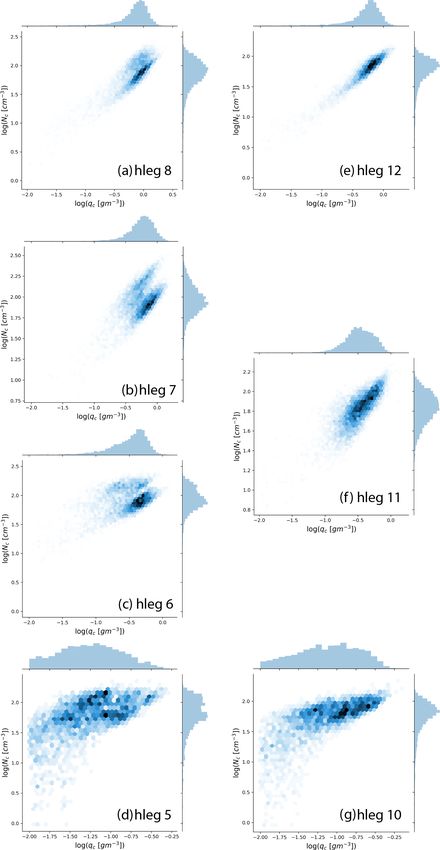
Z. Zhang et al.: Vertical dependence of horizontal variation of cloud microphysics                                                       3107

Figure 1. (a) Horizontal flight track of the G-1 aircraft (red) during the 18 July 2017 RF around the DOE ENA site (yellow star) on Graciosa
Island. (b) The vertical flight track of G-1 (thick black line) overlaid on the radar reflectivity contour by the ground-based KZAR. The dotted
lines in the figure indicate the cloud base and top retrievals from ground-based radar and CEIL instruments. The yellow-shaded regions are
the “hlegs” and green-shaded regions are the “vlegs”. See text for their definitions.

ENA site on Graciosa Island. The average wind in the up-                  As previously mentioned, Boutle et al. (2014) found that the
per MBL (i.e., 900 mbar) is approximately Northwest. So,                  horizontal variance of qc increases with the horizontal scale
the west side of the V-shape horizontal level runs is along the           L slowly when L is larger than about 20 km. Therefore, al-
wind and the east side across the wind. Note that the horizon-            though the horizontal sampling of the selected hlegs is only
tal velocity of the G-1 aircraft is approximately 100 m s−1 .             about 30 km, the lessons learned here could yield useful in-
Since the duration of these selected V-shaped hlegs is be-                sights for larger GCM grid sizes. In addition to the hlegs,
tween 580 and 700 s, their total horizontal length is roughly             we also identified the vertical penetration legs in each flight,
60 km, with each side of the V shape ∼ 30 km. These V-shape               referred to as the “vlegs”, from which we will obtain the ver-
horizontal level runs, with one side along and the other across           tical structure of the MBL, along with the properties of cloud
the wind, are a common sampling strategy used in the ACE-                 and aerosol.
ENA to observe the properties of aerosol and cloud at differ-
ent vertical levels of the MBL. In our study we use the verti-            3.2   Case selection
cal location of the G-1 aircraft from the AIMMS to identify
continuous horizontal flight tracks which are referred to as              As illustrated in Fig. 1a and b for the 18 July 2017 RF, the
the “hlegs”. For the 18 July 2017 case, a total of 13 hlegs               criteria we used to select the RF cases and the hlegs within
are identified as shown in Fig. 1b. Among them, hlegs 5, 6,               the RF can be summarized as follows:
7, 8, 10, 11, and 12 are the seven V-shape horizontal level                  – The RF samples multiple continuous in-cloud hlegs at
runs inside the MBL cloud. Together they provide an excel-                     different vertical levels with the horizontal length of at
lent set of samples of the MBL cloud properties at different                   least 10 km and cloud fraction larger than 10 % (i.e.,
vertical levels of a virtual GCM grid box of about 30 km.                      the fraction of an hleg with qc > 0.01 g m−3 must exceed

https://doi.org/10.5194/acp-21-3103-2021                                                    Atmos. Chem. Phys., 21, 3103–3121, 2021
3108                                     Z. Zhang et al.: Vertical dependence of horizontal variation of cloud microphysics

Table 2. Conditions of MBL sampled during the two IOPs of the ACE-ENA campaign. Dates are given in month and day (m/dd) format.

       Conditions                                                              Research flights
       sampled                           IOP1: June–July 2017                      IOP2: January–February 2018
       Mostly clear                      6/23, 6/29, 7/7                           2/16
       Thin stratus                      6/21, 6/25, 6/26, 6/28, 6/30, 7/4, 7/13   1/28, 2/1, 2/10, 2/12
       Solid stratocumulus               7/6, 7/8, 7/15                            1/30, 2/7
       Multi-layer stratocumulus         7/11, 7/12                                1/24, 1/29, 2/8
       Drizzling stratocumulus/cumulus   7/3, 7/17, 7/18, 7/19, 7/20               1/19, 1/21, 1/25, 1/26, 2/9, 2/11, 2/15, 2/18, 2/19

     10 % of the total length of that hleg). It is important to        4     A study of the 18 July 2017 case
     note here that, unless otherwise specified, all the anal-
     yses of qc and Nc are based on in-cloud observations              4.1    Horizontal and vertical variations of cloud
     (i.e., in the regions with qc > 0.01 g m−3 ).                            microphysics
  – Moreover, the selected hlegs must sample the same re-
    gion (i.e., the same virtual GCM grid box) repeatedly              On 18 July 2017, the North Atlantic is controlled by the Ice-
    in terms of horizontal track but different vertical levels         landic low to the north and the Azores high to the south (see
    in terms of vertical track. Take the 18 July 2017 case as          Fig. 2b), which is a common pattern of large-scale circulation
    an example. The hlegs 5, 6, 7, and 8 follow the same               during the summer season in this region (Wood et al., 2015).
    V-shaped horizontal track (see Fig. 1a) but sample dif-            The Azores is at the southern tip of the cold air sector of a
    ferent vertical levels of the MBL clouds (see Fig. 1b).            frontal system where the fair-weather low-level stratocumu-
    Such hlegs provide us the horizontal sampling needed               lus clouds are dominant (see satellite image in Fig. 2a). The
    to study the subgrid horizontal variations of the cloud            RF on this day started around 08:30 UTC and ended around
    properties and, at the same time, the chance to study the          12:00 UTC. As explained in the previous section, we selected
    vertical dependence of the horizontal cloud variations.            seven hlegs from this RF that horizontally sampled the same
                                                                       region repeatedly in a similar V-shaped track but vertically
  – Finally, the RF needs to have at least one vleg, and the           at different levels. The radar reflectivity observation from the
    cloud boundary derived from the vleg is largely con-               ground-based KAZR during the same period peaks around
    sistent with that derived from the ground-based mea-               10 dBZ, indicating the presence of significant drizzle inside
    surements. This requirement is to ensure that the verti-           the MBL clouds.
    cal locations of the selected hlegs with respect to cloud             Among the seven selected hlegs, hlegs 5, 6, 7, and 8 con-
    boundaries can be specified. For example, as shown                 stitute one set of four consecutive V-shaped tracks, with hlegs
    in Fig. 1b according to the ground-based observations,             5 close to cloud base and hleg 8 close to cloud top. The hlegs
    hlegs 5 and 10 of the 18 July 2017 case are close to               10, 11, and 12 are another set of consecutive V-shaped tracks
    cloud base, while hlegs 8 and 12 are close to cloud top            with hlegs 10 and 12 close to cloud base and top, respec-
    (see also Fig. 4).                                                 tively (see Fig. 1). Using qc > 0.01 g m−3 as a threshold for
                                                                       cloud, the cloud fraction (fc ) of all these hlegs is close to
The above requirements together pose a strong constraint on            unity (i.e., overcast), except for the two hlegs close to cloud
the observation. Fortunately, thanks to the careful planning           base (fc = 46 % for hleg 5 and fc = 51 % for hleg 10). The
of the RF, which had already taken studies like ours into con-         qc and Nc derived from the in situ FCDP measurements for
sideration, we are able to select a total of seven RF cases            these selected hlegs are plotted in Fig. 3 as a function of UTC
as summarized in Table 3. The plots of the flight tracks and           time. It is evident from Fig. 3 that both qc and Nc have signif-
ground-based radar observations for the six other RF cases             icant horizontal variations. At cloud base (see Fig. 3d for hleg
are provided in the Supplement (Figs. S1–S6). We will first            5 and Fig. 3g for hleg 10) the qc varies from 0.01 g m−3 (i.e.,
focus on the golden case – 18 July 2017 RF – and then inves-           the lower threshold) up to about 0.4 g m−3 and the Nc from
tigate if the lessons learned from the 18 July 2017 RF also            25 up to 150 cm−3 , with the mean in-cloud values around
apply to the other three cases.                                        0.08 g m−3 and 65 cm−3 , respectively. Such strong variations
                                                                       of cloud microphysics could be contributed by a number of
                                                                       factors. One can see from the ground radar and lidar obser-
                                                                       vations in Fig. 1b that the height of cloud base varies signif-
                                                                       icantly. As a result, the horizonal legs may not really sample
                                                                       the cloud base. In addition, the variability in updraft at cloud
                                                                       base could lead to the variability in the activation and growth

Atmos. Chem. Phys., 21, 3103–3121, 2021                                                   https://doi.org/10.5194/acp-21-3103-2021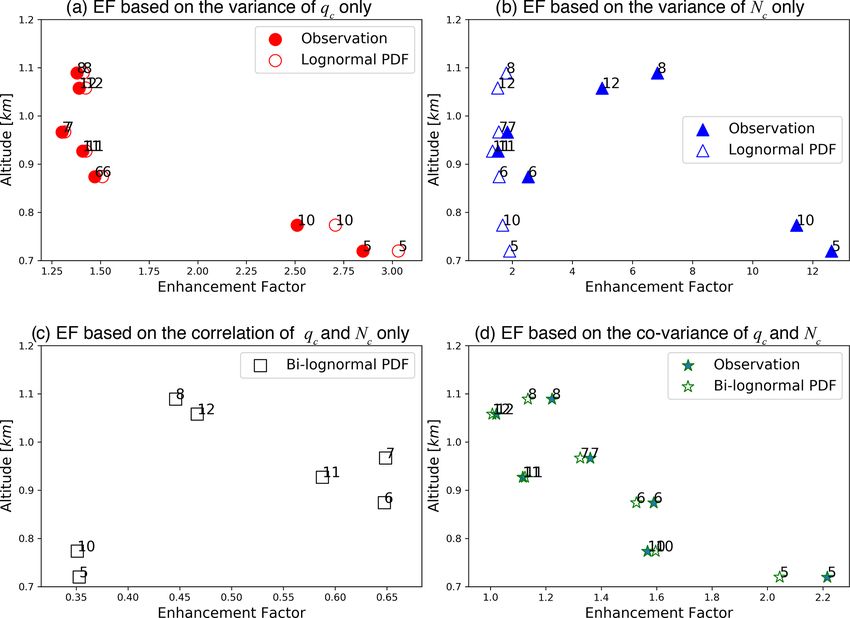
Z. Zhang et al.: Vertical dependence of horizontal variation of cloud microphysics                                                 3109

Table 3. A summary of selected RFs and the selected hlegs and vlegs within each RF.

                 Research flight      Precipitation                       Sampling              Selected hlegs      Selected
                                                                          pattern                                      vlegs
                 13 July 2017         Non-precipitating                   Straight-line                   3, 4, 5     0, 1, 3
                 18 July 2017         Precipitation reaching ground       V shape         5, 6, 7, 8, 10, 11, 12      0, 1, 3
                 20 July 2017         Precipitation reaching ground       V shape          5, 6, 7, 8, 9, 13, 14         0, 1
                 19 January 2018      Precipitation reaching ground       V shape                6, 7, 8, 15, 16      0, 1, 3
                 26 January 2018      Precipitation only at cloud base    Straight-line       3, 4, 5, 9, 10, 11      0, 1, 3
                 7 February 2018      Non-precipitating                   V shape                      1, 2, 3, 5        0, 1
                 11 February 2018     Precipitation reaching ground       Straight-line       4, 5, 6, 7, 12, 13         0, 1

Figure 2. (a) The real color satellite image of the ENA region on 18 July 2017 from MODIS. The small red star marks the location of the
ARM ENA site on Graciosa Island. (b) The averaged sea level pressure (SLP) of the ENA region on 18 July 2017 from the MERRA-2
reanalysis.

of cloud condensation nuclei (CCN). In the middle of the                 of the cloud, i.e., the entrainment zone where the dry air en-
MBL cloud, i.e., hleg 6 (Fig. 3c), 7 (Fig. 3b) and 11 (Fig. 3f),         trained from above mixes with the humid cloudy air in the
the mean value of qc is significantly larger than that of cloud          MBL. In previous studies, a so-called inverse relative vari-
base hlegs while the variability is reduced. The mean value of           ance, ν, is often used to quantify the subgrid variations of
qc keeps increasing toward cloud top to ∼ 0.73 g m−3 in hleg             cloud microphysics. It is defined as follows:
8 (Fig. 3a) and to ∼ 0.53 g m−3 in hleg 12 (Fig. 3e), respec-
tively. In contrast, the horizontal variability of qc seems to                  hxi2
                                                                         νX =        ,                                               (2)
increase in comparison to those observed in mid-level hlegs.                     σX2
   To obtain a further understanding of the vertical variations
of cloud microphysics, we analyzed the cloud microphysics                where X is either qc (i.e., νX = νqc ) or Nc (i.e., νX = νNc )
observations from the two green-shaded vlegs 1 and 3 in                  (Barker et al., 1996; Lebsock et al., 2013; Zhang et al., 2019).
Fig. 1b. The vertical profiles of the mean qc and Nc from                hxi and σX are the mean value and standard deviation of X,
these two vlegs are shown in Fig. 4a and b, respectively, with           respectively. As such, the smaller the ν value, the larger the
the mean and standard deviation of the qc and Nc derived                 horizontal variation of X in comparison to the mean value.
from the seven selected hlegs overplotted. Overall, the ver-             As shown in Fig. 4c, the νqc and νNc derived from the se-
tical profiles of the qc and Nc are qualitatively aligned with           lected hlegs follow a similar vertical pattern: they both in-
the classic adiabatic MBL cloud structure (Brenguier et al.,             crease first from cloud base upward and then decrease in the
2000; Martin et al., 1994). That is, the Nc remains relatively           entrainment zone, with the turning point somewhere around
constant (see Fig. 4b), while the qc increases approximately             1 km (i.e., around hleg 7 and 11). It indicates that both qc
linearly with height from cloud base upward as a result of               and Nc have significant horizontal variabilities at cloud base
condensation growth (see Fig. 4a,), except for the very top              which may be a combined result of horizontal fluctuations
                                                                         of dynamics (e.g., updraft) and thermodynamics (e.g., tem-

https://doi.org/10.5194/acp-21-3103-2021                                                   Atmos. Chem. Phys., 21, 3103–3121, 2021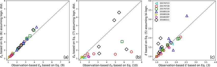
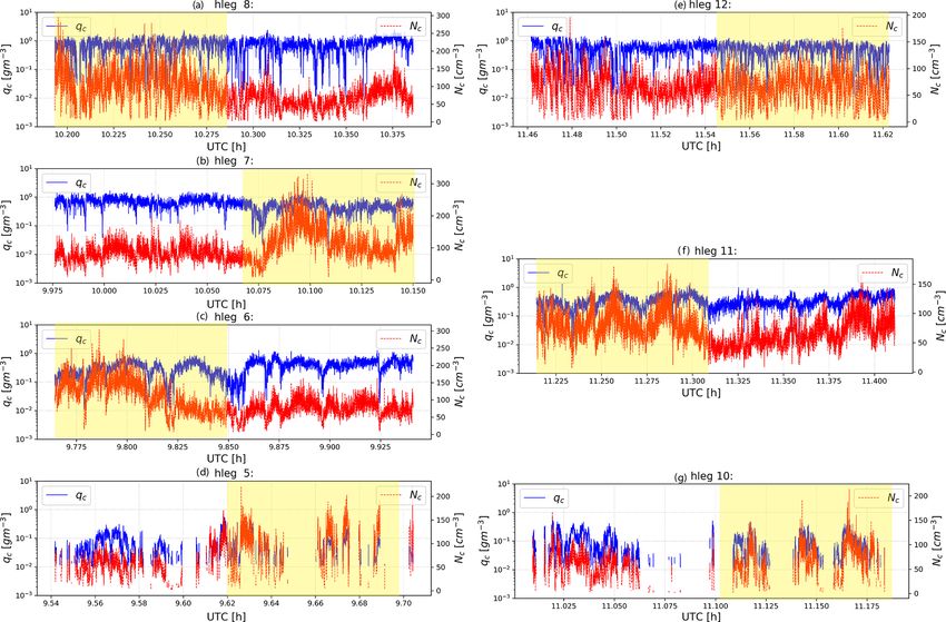
3110                                        Z. Zhang et al.: Vertical dependence of horizontal variation of cloud microphysics

Figure 3. The horizontal variations of qc (red) and Nc (blue) for each selected hleg derived from the in situ FCDP instrument. The yellow-
shaded time period in each plot corresponds to the cross-wind side of the V-shaped flight track, and the unshaded part corresponds to the
along-wind part. Note that plots are ordered such that (a) hleg 8 and (e) hleg 12 are close to cloud top; (b) hleg 6, (c) hleg 7, and (f) hleg 11
are sampled in the middle of clouds; and (d) hleg 5 and (g) hleg 10 are close to cloud base.

perature and dynamics), as well as horizontal variations of                7, and 8 is more complex. As shown in Fig. 5, the joint dis-
aerosols. The horizontal variabilities of both qc and Nc both              tributions of qc and Nc of hleg 6 (Fig. 5b), hleg 7 (Fig. 5c),
decrease upward toward cloud top until the entrainment zone                and, to a less extent, hleg 8 (Fig. 5d) all exhibit a clear bi-
where both variabilities increase again.                                   modality. Further analysis reveals that each of the two modes
   So far, in all the analyses above, the variations of qc and             in these bimodal distributions approximately corresponds to
Nc have been considered separately and independently. As                   one side of the V-shaped track. To illustrate this, the east side
pointed out in several previous studies, the covariation of qc             (i.e., across wind) of the hleg is shaded in yellow in Fig. 3.
and Nc could have an important impact on the EF for the au-                It is intriguing to note that the Nc values from the east side
toconversion process in GCMs (Kogan and Mechem, 2016;                      of the hleg are systematically larger than those from the west
Larson and Griffin, 2013; Zhang et al., 2019). This point will             side, while their qc values are largely similar. It is unlikely
be further elucidated in detail in the next section. Figure 5              that the bimodality is caused by the along-wind and across-
shows the joint distributions of qc and Nc for the seven se-               wind difference between the two sides of the V-shaped track.
lected hlegs, and the corresponding linear correlation coeffi-             It is most likely just a coincidence. On the other hand, the
cients as a function of height are shown in Fig. 4d. For the               bimodal joint distribution between qc and Nc is real, which
sake of reference, the linear correlation coefficient between              could be a result of subgrid variations of updraft, precipita-
ln(qc ) and ln(Nc ) , i.e., the ρL that will be introduced later in        tion, and/or aerosols.
Eq. (4), is also plotted in Fig. 4d. Looking first at hlegs 10, 11,           As a result of the bimodality of Nc , the correlation coef-
and 12, i.e., the second group of consecutive V-shaped legs,               ficients between qc and Nc is significantly smaller for hlegs
there is a clear increasing trend of the correlation between qc            6 (ρ = 0.22) and 7 (ρ = 0.31) in comparison to other hlegs.
and Nc from cloud bottom (ρ = 0.75 for hleg 10) to cloud                   However, if the two sides of the V-shaped tracks are con-
top (ρ = 0.95 for hleg 12). The picture based on hlegs 5, 6,               sidered separately, then qc and Nc become more correlated,

Atmos. Chem. Phys., 21, 3103–3121, 2021                                                       https://doi.org/10.5194/acp-21-3103-2021
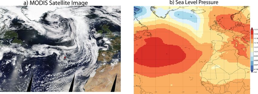
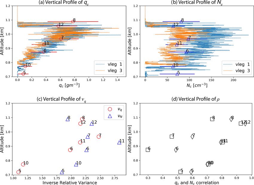
Z. Zhang et al.: Vertical dependence of horizontal variation of cloud microphysics                                                           3111

Figure 4. (a) The vertical profiles of qc derived from the vlegs (dotted lines) of the 18 July 2017 case. The overplotted red error bars indicate
the mean values and standard deviations of the qc derived from the selected hlegs at different vertical levels. (b) Same as panel (a) except
for Nc . (c) The vertical profile of the inverse relative variances (i.e., mean divided by standard deviation) of Nc (red circle) and Nc (blue
triangle) derived from the hleg; (d) the vertical profile of the linear correlation coefficient between ln(qc ) and ln(Nc ), i.e., ρL (square), and
the linear correlation coefficient between qc and Nc , i.e., ρ (diamond).

except for the east side of hleg 6, which still exhibits to some            from Fig. 1 the selected hlegs are sampled at different ver-
degree a bimodal joint distribution of qc and Nc . In spite of              tical locations and also at different times. For example, hleg
the bimodality, there is evidently a general increasing trend               5 at cloud base is more than 1 h apart from hleg 8 at cloud
of the correlation between qc and Nc from cloud base toward                 top (Fig. 1a). As a result, the temporal evolution of clouds
cloud top. At the cloud top, the qc and Nc correlation coeffi-              is a confounding factor and might be misinterpreted as verti-
cient can be as high as ρ = 0.95 for hleg 12 (see Fig. 5e). As              cal variations of clouds. On the other hand, as shown below,
explained in the next section, this close correlation between               we also observed similar vertical structure of qc and Nc in
qc and Nc has important implications for the simulation of                  other cases. It seems highly unlikely that the temporal eval-
the autoconversion enhancement factor.                                      uations of the clouds in all selected cases conspire to con-
   As a summary, the above phenomenological analysis of                     found our results in the same way. Based on this considera-
the 18 July 2017 RF reveals the following features of the                   tion, we assume that the temporal evolution of clouds is an
horizontal and vertical variations of cloud microphysics. Ver-              uncertainty that could lead to random errors but does not im-
tically, the mean values of qc and Nc qualitatively follow the              pact the overall vertical trend. The second caveat is that due
adiabatic structure of MBL cloud; i.e., qc increases linearly               to the very limited vertical sampling rate of hlegs (i.e., only
with height and Nc remains largely invariant above cloud                    3–4 samples), we cannot possibly resolve the detailed verti-
base. Even though the joint distribution of qc and Nc ex-                   cal variation of νq , νN , and ρ. Although we have used the
hibits a bimodality in several hlegs, their correlation gener-              word “trend” in the above analysis, it should be noted that
ally increases with height and can be as high as ρ = 0.95 at                the vertical profile of these parameters may, but more likely
cloud top. Horizontally, both qc and Nc have a significant                  may not, be linear. So, the word “trend” here indicates only
variability at cloud base, which tends to first decrease up-                the large pattern that can be resolved by the hlegs. Obviously
ward and then increase in the uppermost part of cloud close                 these two caveats also apply to the analysis below the EF,
to the entrainment zone. Finally, we have to point out a cou-               which is also derived from the hlegs.
ple of important caveats in the above analysis. First, as seen

https://doi.org/10.5194/acp-21-3103-2021                                                       Atmos. Chem. Phys., 21, 3103–3121, 2021
3112                                         Z. Zhang et al.: Vertical dependence of horizontal variation of cloud microphysics

Figure 5. The joint distributions of qc and Nc , along with the marginal histograms, for the seven selected hlegs from the 18 July 2017 RF.
As in Fig. 3, the plots are ordered such that (a) hleg 8 and (e) hleg 12 are close to cloud top; (b) hleg 6, (c) hleg 7, and (f) hleg 11 are sampled
in the middle of clouds; and (d) hleg 5 and (g) hleg 10 are close to cloud base.

Atmos. Chem. Phys., 21, 3103–3121, 2021                                                         https://doi.org/10.5194/acp-21-3103-2021
Z. Zhang et al.: Vertical dependence of horizontal variation of cloud microphysics                                               3113

4.2   Implications for the EF for the autoconversion rate            where Eq νqc , βq corresponds to the enhancing effect of
      parameterization                                               the subgrid variation of qc , if qc follows a marginal lognor-
                                                                                                                       x−µ)2

                                                                     mal distribution, i.e., P (x) = √ 1 exp − (ln 2σ    2     . It is
As explained in the introduction, in GCMs the autoconver-                                               2πxσ
                                                                     a function of the inverse relative variance νq in Eq. (2) as
sion process is usually parameterized as a highly nonlinear
                                                                     follows:
function of qc and Nc , e.g., the KK scheme in Eq. (1). In
such a parameterization, an EF is needed to account for the                                           βq2 −βq
                                                                                                1          2
bias caused by the nonlinearity effect. A variety of methods

                                                                     E q ν qc , β q       = 1+                     .               (6)
have been proposed and used in the previous studies to esti-                                   νqc
mate the EF (Larson and Griffin, 2013; Lebsock et al., 2013;
                                                                     Similarly, the EN νNc , βN below corresponds to the en-
Pincus and Klein, 2000; Zhang et al., 2019). The methods             hancing effect of the subgrid variation of Nc , if Nc follows a
used in this study are based on Z19. Only the most relevant          marginal lognormal distribution:
aspects are recapped here. Readers are referred to Z19 for
                                                                                                               2
detail.                                                                                                  βN −βN
                                                                                                   1              2
   If the subgrid variations of qc and Nc , as well as their co-     EN vNc , βN              = 1+                     .           (7)
variation, are known, then the EF can be estimated based on                                        νNc
its definition as follows:

                                                                     The third term ECOV ρL , βq , βN νqc , νNc in Eq. (5),
       R ∞ R ∞ βq βN
        N     q     qc Nc P (qc , Nc ) dqc dNc                       ECOV ρL , βq , βN , vqc , vNc = exp ρL βq βN σqc σNc ,        (8)
E = c,min c,min                                ,             (3)
                    hqc iβq hNc iβN                                  corresponds to the impact of the covariation of qc and Nc on
                                                                     the EF. Because βq > 0 and βN < 0, if qc and Nc are neg-
where hqc i and hNc i are the grid-mean value, P (qc , Nc ) is the
                                                                     atively correlated (i.e., ρL < 0), then the ECOV > 1 and acts
joint probability density function (PDF) of qc and Nc . qc,min
                                                                     as an enhancing effect on the autoconversion rate computa-
and Nc,min are the lower limits of the in-cloud value (e.g.,
                                                                     tion. In contrast, if qc and Nc are positively correlated (i.e.,
qc,min = 0.01 g m−3 ). Some previous studies approximate the
                                                                     ρL > 0), then the ECOV < 1, which becomes a suppressing
P (qc , Nc ) as a bivariate lognormal distribution as follows:
                                                                     effect on the autoconversion rate computation.
                                                                        As previously mentioned, most previous studies of the EF

                             1                   ζ
P (qc , Nc ) =                   q       exp −                       consider only the impact of subgrid qc variation (i.e., only
                2π qc Nc σqc σNc 1 − ρL2         2
                                                                     the Eq term). The impacts of subgrid Nc variation as well
              "                                                     as its covariation with qc have been largely overlooked in
                  ln qc − µqc 2

         1
ζ=                                                                   observational studies, in which the Eq is often derived from
     1 − ρL2          σqc                                            the observed subgrid variation of qc based on the definition
                                                                     of EF, i.e.,

            ln qc − µqc      ln Nc − µNc
   −2ρ
                σqc              σNc                                        R ∞ βq
                                                                             q    qc P (qc ) dqc

        ln Nc − µNc
                      2 #                                           Eq = c,min                  ,                               (9)
   +                       ,                                   (4)                 hqc iβq
             σNc
                                                                     where P (qc ) is the observed subgrid PDF of qc . Alterna-
where µX and σX are, respectively, the mean and standard             tively, Eq has also been estimated from the inverse relative
deviation of ln(X), where X is either qc or Nc . ρL is the lin-      variance νq by assuming the subgrid variation of qc fol-
ear correlation coefficient between ln(qc ) and ln(Nc ) (Larson      lows the lognormal distribution, in which case Eq is given
and Griffin, 2013; Lebsock et al., 2013; Zhang et al., 2019). It     in Eq. (6).
should be noted here that ρL is fundamentally different from            Similar to EN , if only the effect of subgrid Nc is consid-
ρ (i.e., the linear correlation coefficient between qc and Nc ).     ered, the corresponding EN can be derived from the follow-
On the other hand, we found that for all the selected hlegs,         ing two ways: one from the observed subgrid PDF P (Nc )
ρ and ρL are in an excellent agreement (see Fig. 4d). In fact,       based on the definition of EF, i.e.,
ρ and ρL can be used interchangeably in the context of this                  R∞      β
                                                                                   Nc N P (Nc ) dNc
                                                                              N
study without any impact on the conclusions. Nevertheless,           EN = c,min                     ,                          (10)
interested readers may find more detailed discussion of the                         hNc iβN
relationship between ρ and ρL in Larson and Griffin (2013).          and the other based on Eq. (7) from the relative variance νNc
   Substituting P (qc , Nc ) in Eq. (4) into Eq. (3) yields a for-   by assuming the subgrid Nc variation follows the lognormal
mula for EF that consists of the following three terms:              distribution.
                                                                      Now, we put the in situ qc and Nc observations from the
E = Eq νqc , βq · EN νNc , βN                                        selected hlegs in the theoretical framework of EF described

   · ECOV ρL , βq , βN νqc , νNc ,                             (5)   above and investigate the following questions:

https://doi.org/10.5194/acp-21-3103-2021                                                       Atmos. Chem. Phys., 21, 3103–3121, 2021
3114 Z. Zhang et al.: Vertical dependence of horizontal variation of cloud microphysics
1. What is the (observation-based) EF derived based on The Eq and EN reflect only the individual contributions
Eq. (3) from the observed joint PDF P (qc , Nc )? of subgrid qc and Nc variations to the EF. The effect of the
covariation of qc and Nc , i.e., the ECOV , is shown in Fig. 6c.
2. How well does the (bi-logarithmic) EF derived based Interestingly, the value of ECOV is smaller than unity for all
on Eq. (5) by assuming that the covariation of qc the selected hlegs. As explained in Eq. (8), ECOV < 1 is a re-
and Nc follows a bivariate lognormal agree with the sult of a positive correlation between qc and Nc , as seen in
observation-based EF? Fig. 4d. Therefore, in these hlegs the covariation of the qc and
Nc has a suppressing effect on the EF, in contrast to the en-
3. What is the relative importance of the Eq , EN , and hancing effect of Eq and EN . This result is qualitatively con-
ECOV terms in Eq. (5) in determining the value of EF? sistent with Z19, who found that the vertically integrated liq-
uid water path (LWP) of MBL clouds is in general positively
4. What is the error of considering only Eq and omitting
correlated with the Nc estimated from the MODIS cloud re-
the EN and ECOV terms?
trieval product and, as a result, ECOV < 1 over most of the
5. How do the observation-based EFs from Eq. (3) and the tropical oceans. Because of the relationship in Eq. (8), the
Eq , EN , and ECOV terms vary with vertical height in value ECOV is evidently negatively proportional to the corre-
cloud? lation coefficient ρL in Fig. 4d. The largest value is seen in
hleg 6 and 7, in which the bimodal joint distribution of qc and
These questions are addressed in the rest of this section. Nc results in a small ρL . A rather small value of ECOV ∼ 0.45
Focusing first on the Eq in Fig. 6a, the Eq derived from is seen for cloud top hleg 8 and 12, as result of a strong cor-
observation based on Eq. (9) (solid circle) shows a clear relation between qc and Nc (ρL > 0.9) and moderate σq and
decreasing trend with height between cloud base at around σN .
700 m to about 1 km, with a value reduced from about 3 to Finally, the EF that accounts for all factors, including the
about 1.2. Then, the value of Eq increases slightly in the individual variations of qc and Nc , as well as their covaria-
cloud top hlegs 8 and 12. The Eq derived based on Eq. (6) tion, is shown in Fig. 6d. Focusing first on the observation-
by assuming lognormal distribution (open circle) has a very based results (solid star), i.e., E in Eq. (3), evidently there is
similar vertical pattern, although the value is slightly overes- a decreasing trend from cloud base (e.g., E = 2.2 for hleg
timated on average by 0.07 in comparison to the observation- 5 and E = 1.59 for hleg 10) to cloud top (e.g., E = 1.20
based result. The vertical pattern of Eq can be readily ex- for hleg 8 and E = 1.02 for hleg 12). The E values derived
plained by the subgrid variation of qc in Fig. 4c. The EN based on Eq. (5) by assuming the bivariate lognormal dis-
derived from observation (solid triangle) in Fig. 6b shows a tribution between qc and Nc (i.e., open star in Fig. 6d) are
similar vertical pattern as Eq , i.e., first decreasing with height in reasonable agreement with the observation-based results,
from cloud base to about 1.2 km and then increasing with with a mean bias of −0.09. It is intriguing to note that the
height in the uppermost part of cloud. The EN derived based value of E = Eq ·EN ·ECOV in Fig. 6d is comparable to Eq in
on Eq. (7) by assuming a lognormal distribution (open trian- Fig. 6a, which indicates that the enhancing effect of EN > 1
gle) significantly underestimates the observation-based val- in Fig. 6b is partially canceled by the suppressing effect of
ues (mean bias of −4.3), especially at cloud base (i.e., hleg 5 ECOV < 1 in Fig. 6c. As previously mentioned, many pre-
and 10) and cloud top (i.e., hleg 8 and 12). vious studies of the EF consider only the effect of Eq but
Using hleg 10 as an example, we further investigated the overlook the effect of EN and ECOV . The error in the stud-
cause for the error in lognormal-based EFs in comparison to ies would be quite large if it were not for a fortunate error
those diagnosed from the observation. As shown in Fig. 7a cancellation.
the observed qc is slightly negatively skewed in logarithmic
space by the small values. Because the autoconversion rate is
proportional to qc2.47 , the negatively skewed qc also leads to a 5 Other selected cases
negatively skewed Eq in Fig. 7b. As a result, the leg-averaged
In addition to the 18 July 2017 RF, we also found another
Eq diagnosed from the observation is slightly smaller than
six RFs that meet our criteria as described in Sect. 3 for case
that derived based on Eq. (6) by assuming a lognormal dis-
selection, from non-precipitating (e.g., 13 July 2017 case in
tribution. The negative skewness also explains the large error
Fig. S1) to weakly (e.g., 26 January 2018 case in Fig. S4)
in EN for hleg 10 seen on Fig. 6b. As shown in Fig. 7c the
and heavily precipitating cloud (11 February 2018 case in
observed Nc is also negatively skewed to a much larger ex-
Fig. S6). Due to limited space, we cannot present the detailed
tent in comparison to qc . Because the autoconversion rate is
case studies of these RFs. Instead, we view them collectively
proportional to Nc−1.79 , the highly negatively skewed Nc re-
and investigate whether the lessons learned from the 18 July
sults in a highly positively skewed EN in Fig. 7d. As a result,
2017 RF, especially those about the EF in Sect. 4.2, also ap-
the EN diagnosed from the observation is much larger than
ply to the other cases.
that derived based on Eq. (7) by assuming a lognormal dis-
tribution.
Atmos. Chem. Phys., 21, 3103–3121, 2021 https://doi.org/10.5194/acp-21-3103-2021Z. Zhang et al.: Vertical dependence of horizontal variation of cloud microphysics 3115
Figure 6. (a) Eq as a function of height derived from observation based on Eq. (9) (solid circle) and from the inverse relative variance νq
assuming lognormal distribution based on Eq. (6) (open circle). (b) EN as a function of height derived from observation based on Eq. (10)
(solid triangle) and from the inverse relative variance νN assuming lognormal distribution based on Eq. (7) (open triangle). (c) ECOV derived
based on Eq. (8) as a function of height. (d) E as a function of height derived from observation based on Eq. (3) (solid star) and based on
Eq. (5) assuming a bi-lognormal distribution (open star). The numbers beside the symbols in the figure correspond to the numbers of the
seven selected hlegs.
In order to compare the hlegs from different RFs, we first the 18 July 2017 case in Fig. 6a and b. Note that the Eq and
normalize the altitude of each hleg with respect to the min- EN are influenced by a number of factors, such as horizon-
imum and maximum values of all selected hlegs in each RF tal distance and cloud fraction, in addition to vertical height.
as follows: It is possible that the differences in other factors outweigh
zhleg − zmin the vertical dependence here. Interestingly, the linear cor-
∗
zhleg = , (11) relation coefficient ρ between qc and Nc in Fig. 8d shows
zmax − zmin ∗
an increasing trend with zhleg that is statistically significant
∗
where zhleg is the normalized altitude for each hleg in a RF, (R value = 0.50 and P value = 0.02), despite a few outliers.
and zmin and zmax are the altitude of the lowest and high- This is consistent with what we found in the 18 July 2017
est hleg in the corresponding RF. Defined this way, zhleg ∗ is case (see Fig. 4d). As evident from Eq. (8), an increase in
∗
bounded between 0 and 1. Alternatively, zhleg could also be ρL would lead to a decrease in ECOV . Since neither Eq nor
defined with respect to the averaged cloud top (ztop ) and base EN shows a clear dependence on zhleg ∗ , the decrease in E
COV
(zbase ) as inferred from the KAZR or vlegs. However, be- ∗
with zhleg seems to play an important role in the determin-
cause of the variation of cloud top and cloud base heights, ing the value of E. Another line of evidence supporting this
∗
as well as the collocation error, the zhleg would often become role is the fact that both Eq and EN are quite large for the
∗
significantly larger than 1 or smaller than 0, if zhleg were de- cloud top hlegs, while in contrast the values of the corre-
fined with respect to ztop and zbase , making results confusing sponding E that accounts for the covariation of qc and Nc
and difficult to interpret. are much smaller. For example, the Eq for two hlegs from
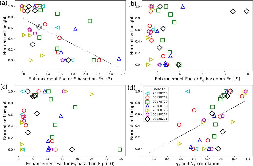
Figure 8 shows the observation-based EFs for all the se- the 11 February 2018 RF exceeds 8, but the corresponding
lected hlegs from the seven selected RFs as a function of the E values are smaller than 1.2, which is evidently a result of
∗ . As shown in Fig. 8a, the E derived based on Eq. (3)
zhleg large ρL and thereby small ECOV .
that accounts for the covariation of qc and Nc has a decreas- As previously mentioned, many previous studies of the EF
ing trend from cloud base to cloud top. This is consistent for the autoconversion rate parameterization consider only
with the result from the 18 July 2017 case in Fig. 6d. How- the effect of subgrid qc variation but ignore the effects of sub-
ever, neither the Eq in Fig. 8b nor the EN in Fig. 8c shows grid Nc variation and its covariation with qc . To understand
a clear dependence on zhleg ∗ in comparison to the results of
https://doi.org/10.5194/acp-21-3103-2021 Atmos. Chem. Phys., 21, 3103–3121, 20213116 Z. Zhang et al.: Vertical dependence of horizontal variation of cloud microphysics
Figure 7. (a) Histogram of ln(qc ) based on observations from hleg 10 (bars) and the lognormal PDF (dashed line) based on the µqc and
σqc of hleg 10. (b) The histogram of ln(Eq ) diagnosed from the observed qc based on Eq. (9). The two vertical lines correspond to the
leg-averaged ln(Eq ) derived based on the observed qc (solid) and the lognormal PDF (dashed line), respectively. (c) Histogram of ln(Nc )
based on observations from hleg 10 (bars) and the lognormal PDF (dashed line) based on the µNc and σNc of hleg 10. (d) The histogram of
ln(EN ) diagnosed from the observed qc based on Eq. (10). The two vertical lines correspond to the leg-averaged ln(EN ) derived based on
the observed Nc (solid) and the lognormal PDF (dashed line), respectively.
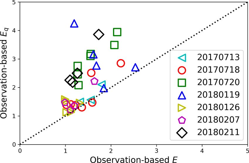
the potential error, we compared the Eq and E both derived Nc PDF from the lognormal distribution is probably the rea-
based on observations in Fig. 9. Apparently, Eq is signifi- son for the large difference of EN in Fig. 10b. As shown in
cantly larger than E for most of the selected hlegs, which im- Fig. 10c, the E values derived based on Eq. (5) by assum-
plies that considering only subgrid qc variation would likely ing a bivariate lognormal function for the joint distribution
lead to an overestimation of EF. This is an interesting re- of qc and Nc are in good agreement with observation-based
sult. Note that EN ≥ 1 by definition and therefore Eq > E is values, which is consistent with the results from the 18 July
possible only when the covariation of qc and Nc has a sup- 2017 case in Fig. 6.
pressing effect, instead of enhancing. Once again, this result
demonstrates the importance of understanding the covaria-
tion of qc and Nc for understanding the EF for autoconver- 6 Summary and discussion
sion rate parameterization.
Having looked at the observation-based EFs, we now In this study we derived the horizontal variations of qc and
check if the EFs derived based on assumed PDFs (e.g., log- Nc , as well as their covariations in MBL clouds based on the
normal or bivariate lognormal distributions) agree with the in situ measurements from the recent ACE-ENA campaign,
observation-based results. As shown in Fig. 10a, the Eq and investigated the implications of subgrid variability as it
based on Eq. (6) that assumes a lognormal distribution for relates to the enhancement of autoconversion rates. The main
the subgrid variation of qc is in an excellent agreement with findings can be summarized as follows:
the observation-based results. In contrast, the comparison is
much worse for the EN in Fig. 10b, which is not surprising – In the 18 July 2017 case, the vertical variation of the
given the results from the 18 July 2017 case in Fig. 6b. As one mean values of qc and Nc roughly follows the adiabatic
can see from Fig. 5, the marginal PDF of Nc is often broad structure. The horizontal variances of qc and Nc first de-
and sometimes even bimodal. The deviation of the observed crease from cloud base upward toward the middle of the
cloud and then increase near cloud top. The correlation
Atmos. Chem. Phys., 21, 3103–3121, 2021 https://doi.org/10.5194/acp-21-3103-2021You can also read