Photo-astrometric distances, extinctions, and astrophysical parameters for Gaia DR2 stars brighter than G = 18
←
→
Page content transcription
If your browser does not render page correctly, please read the page content below
Astronomy & Astrophysics manuscript no. GDR2_SH                                                                                       c ESO 2019
                                              July 4, 2019

                                                        Photo-astrometric distances, extinctions, and astrophysical
                                                            parameters for Gaia DR2 stars brighter than G = 18
                                                     F. Anders1, 2, 3 , A. Khalatyan2 , C. Chiappini2, 3 , A. B. Queiroz2, 3 , B. X. Santiago4, 3 , C. Jordi1 , L. Girardi5 ,
                                                  A. G. A. Brown6 , G. Matijevič2 , G. Monari2 , T. Cantat-Gaudin1 , M. Weiler1 , S. Khan7 , A. Miglio7 , I. Carrillo2 ,
                                                         M. Romero-Gómez1 , I. Minchev2 , R. S. de Jong2 , T. Antoja1 , P. Ramos1 , M. Steinmetz2 , H. Enke2

                                                    1
                                                        Institut de Ciències del Cosmos, Universitat de Barcelona (IEEC-UB), Carrer Martí i Franquès 1, 08028 Barcelona, Spain
                                                        e-mail: fanders@icc.ub.edu
                                                    2
                                                        Leibniz-Institut für Astrophysik Potsdam (AIP), An der Sternwarte 16, 14482 Potsdam, Germany
                                                    3
                                                        Laboratório Interinstitucional de e-Astronomia - LIneA, Rua Gal. José Cristino 77, Rio de Janeiro, RJ - 20921-400, Brazil
                                                    4
arXiv:1904.11302v3 [astro-ph.GA] 3 Jul 2019

                                                        Instituto de Física, Universidade Federal do Rio Grande do Sul, Caixa Postal 15051, Porto Alegre, RS - 91501-970, Brazil
                                                    5
                                                        Osservatorio Astronomico di Padova, INAF, Vicolo dell’Osservatorio 5, 35122 Padova, Italy
                                                    6
                                                        Leiden Observatory, P.O. Box 9513, 2300 RA, Leiden, The Netherlands
                                                    7
                                                        School of Physics and Astronomy, University of Birmingham, Edgbaston, Birmingham, B 15 2TT, United Kingdom
                                                   Received 25.04.2019; accepted 27.06.2019

                                                                                                                ABSTRACT

                                                   Combining the precise parallaxes and optical photometry delivered by Gaia’s second data release (Gaia DR2) with the photometric
                                                   catalogues of Pan-STARRS1, 2MASS, and AllWISE, we derived Bayesian stellar parameters, distances, and extinctions for 265
                                                   million of the 285 million objects brighter than G = 18. Because of the wide wavelength range used, our results substantially improve
                                                   the accuracy and precision of previous extinction and effective temperature estimates. After cleaning our results for both unreliable
                                                   input and output data, we retain 137 million stars, for which we achieve a median precision of 5% in distance, 0.20 mag in V-
                                                   band extinction, and 245 K in effective temperature for G ≤ 14, degrading towards fainter magnitudes (12%, 0.20 mag, and 245
                                                   K at G = 16; 16%, 0.23 mag, and 260 K at G = 17, respectively). We find a very good agreement with the asteroseismic surface
                                                   gravities and distances of 7000 stars in the Kepler, K2-C3, and K2-C6 fields, with stellar parameters from the APOGEE survey,
                                                   and with distances to star clusters. Our results are available through the ADQL query interface of the Gaia mirror at the Leibniz-
                                                   Institut für Astrophysik Potsdam (gaia.aip.de) and as binary tables at data.aip.de. As a first application, we provide distance-
                                                   and extinction-corrected colour-magnitude diagrams, extinction maps as a function of distance, and extensive density maps. These
                                                   demonstrate the potential of our value-added dataset for mapping the three-dimensional structure of our Galaxy. In particular, we see a
                                                   clear manifestation of the Galactic bar in the stellar density distributions, an observation that can almost be considered direct imaging
                                                   of the Galactic bar.
                                                   Key words. Galaxy: general – Galaxy: abundances – Galaxy: disk – Galaxy: evolution – Galaxy: stellar content – Stars: abundances

                                              1. Introduction                                                            et al. 2018), astrophysical parameters for ' 108 stars (Andrae
                                                                                                                         et al. 2018), and radial velocities for 7 · 106 of them (Sartoretti
                                              Galactic astrophysics is currently in a similar phase as geography         et al. 2018; Katz et al. 2019).
                                              was in the 15th century: large parts of the Earth were unknown to              The Gaia DR2 dataset thus represents a treasure trove for
                                              contemporary scientists, only crude maps of most of the known              many branches of Galactic astrophysics. Various advances have
                                              parts of the Earth existed, and even the orbit of our planet was           since been achieved in the field of Galactic dynamics (e.g. Gaia
                                              still under debate. Nowadays, major parts of the Milky Way are             Collaboration et al. 2018c,d; Antoja et al. 2018; Kawata et al.
                                              still hidden by thick layers of dust, but we are beginning to dis-         2018; Quillen et al. 2018; Ramos et al. 2018; Laporte et al.
                                              cover and to map our Galaxy in a much more accurate fashion                2019; Monari et al. 2019; Trick et al. 2019), star clusters and as-
                                              by virtue of dedicated large photometric, astrometric, and spec-           sociations (e.g. Gaia Collaboration et al. 2018a; Cantat-Gaudin
                                              troscopic surveys.                                                         et al. 2018; Cantat-Gaudin et al. 2018a,b; Castro-Ginard et al.
                                                  In this context, the astrometric European Space Agency mis-            2018; Soubiran et al. 2018; Zari et al. 2018; Baumgardt et al.
                                              sion Gaia (Gaia Collaboration et al. 2016) represents a major              2019; Bossini et al. 2019; de Boer et al. 2019; Meingast & Alves
                                              leap in our understanding of the Milky Way’s stellar content: its          2019), the Galactic star-formation history (Helmi et al. 2018;
                                              measurement precision as well as the absolute number counts                Mor et al. 2019), hyper-velocity stars (e.g. Bromley et al. 2018;
                                              surpass previous astrometric datasets by several orders of mag-            Scholz 2018; Shen et al. 2018; Boubert et al. 2018, 2019; Erkal
                                              nitude. The recent Gaia Data Release 2 (Gaia DR2; Gaia Collab-             et al. 2019), among others. Apart from stellar science, the pre-
                                              oration et al. 2018b), covered the first 22 months of observations         cise Gaia DR2 photometry, in combination with the high quality
                                              (from a currently predicted total of approximately ten years) with         of the stellar parallax measurements, can also be used to map
                                              positions and photometry for 1.7·109 sources (Evans et al. 2018),          the distribution of dust in the Galaxy. The availability of pre-
                                              proper motions and parallaxes for 1.3 · 109 sources (Lindegren             cise individual distance and extinction determinations (mainly
                                                                                                                                                                    Article number, page 1 of 32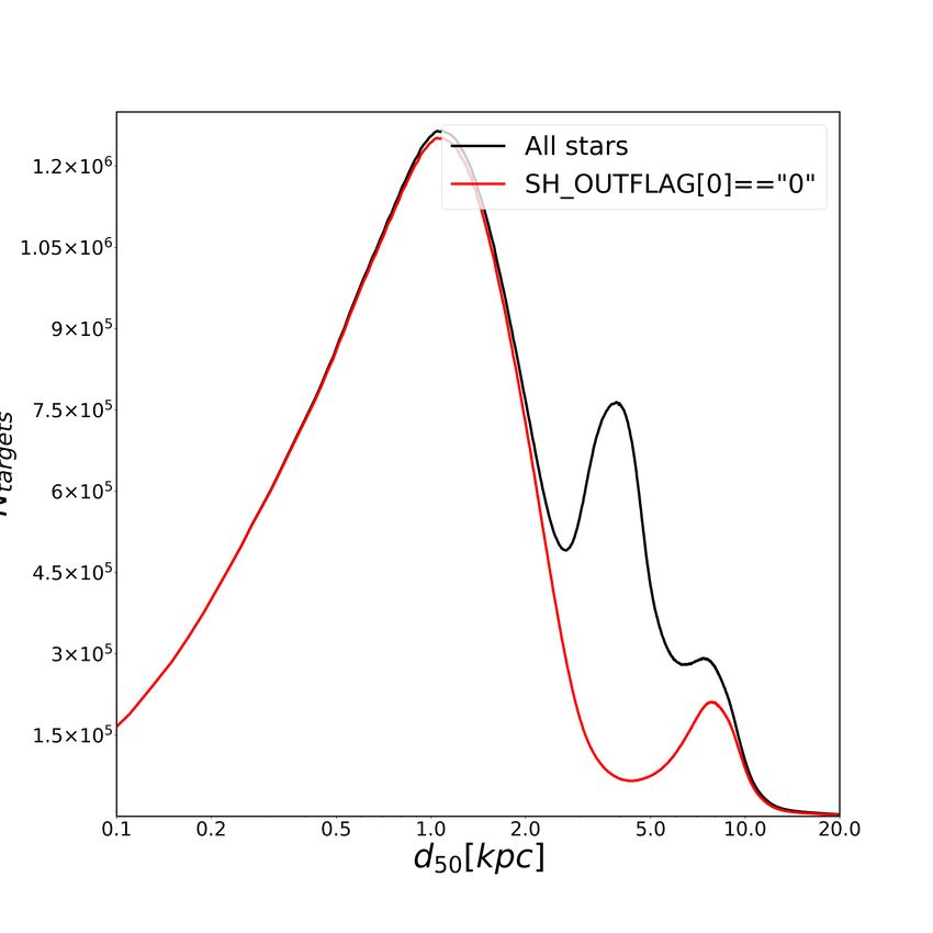
A&A proofs: manuscript no. GDR2_SH

Table 1. Summary of calibrations and data curation applied for fiducial StarHorse run. Details are provided in Sect. 2.

 Parameter        Parameter regime         Calibration choice                                                Reference
                       G < 14              parallax + 0.05 mas                                               Lindegren (2018); Zinn et al. (2019)
    $cal           14 < G < 16.5           parallax + (0.1676 − 0.0084 · phot_g_mean_mag) mas                Lindegren (2018), linear interpolation
                      G > 16.5             parallax + 0.029 mas                                              Lindegren et al. (2018)
                       G < 11              1.2 · parallax_error
     σcal
      $             11 < G < 15            (0.22 · phot_g_mean_mag − 1.22) · parallax_error                  Fit to Lindegren (2018) data
                       G > 15              (e−(phot_g_mean_mag−15) + 1.08) · parallax_error
                       G 16              phot_g_mean_mag − 0.032
                     G < 10.87             using bright GBP filter curve
    GBP                                                                                                      Maíz Apellániz & Weiler (2018)
                     G > 10.87             using faint GBP filter curve
    gPS1                                   g_mean_psf_mag − 0.020
    rPS1                                   r_mean_psf_mag − 0.033
    iPS1               G > 14              i_mean_psf_mag − 0.024                                            Scolnic et al. (2015)
    zPS1                                   z_mean_psf_mag − 0.028
    yPS1                                   y_mean_psf_mag − 0.011
                Gaia, 2MASS, WISE          max{σmag,source , 0.03mag}
    σmag
                  Pan-STARRS1              max{σmag,source , 0.04mag}

from high-resolution spectroscopic surveys, and also recently            giant stars. Although the data quality degrades notably around
from Gaia) has led to a significant improvement of interstellar          a magnitude of G ∼ 16.5, we provide useful information for
dust maps within the past years and months (e.g. Lallement et al.        considerable fraction of stars down to G = 18. To this end, we
2014; Green et al. 2015; Capitanio et al. 2017; Rezaei Kh. et al.        use the python code StarHorse, originally designed to deter-
2017, 2018; Lallement et al. 2018; Lallement et al. 2019; Yan            mine stellar parameters and distances for spectroscopic surveys
et al. 2019, Leike & Enßlin 2019; Chen et al. 2019).                     (Santiago et al. 2016; Queiroz et al. 2018).1 Of the 285 million
     In addition to the main Gaia DR2 data products (paral-              objects with G ≤ 18 contained in Gaia DR2, our code delivered
laxes, proper motions, radial velocities, and photometry), the           results for ∼ 266 million stars. Applying a number of conserva-
Gaia DR2 data allowed for the immediate computation of quan-             tive quality criteria on the input and output data, we achieve a
tities relevant for Galactic stellar population studies. These are       sample cleaned on the basis of data quality flags (see Sect. 3.4)
the Bayesian geometric distance estimates computed by Bailer-            of around 137 million stars with reliable stellar parameters, dis-
Jones et al. (2018) and the first stellar parameters and extinc-         tances, and extinctions.
tion estimates from the Gaia Apsis pipeline (Andrae et al. 2018).            The paper is structured as follows: Section 2 presents the in-
The latter authors deliberately used only Gaia DR2 data prod-            put data used in the parameter estimation. The following Sect.
ucts to infer line-of-sight extinctions as well as effective tem-        3 describes the basics of our code, focussing on updates with
peratures, radii, and luminosities. This proved to be a difficult        respect to its previous applications to spectroscopic stellar sur-
exercise since the three broad Gaia passbands contain little in-         veys. Section 3.4 in particular explains how we flagged the
formation to discriminate between effective temperature and in-          StarHorse results for Gaia DR2. Since we decided to provide
terstellar extinction. As a result, the Apsis T eff estimates were       results for all objects that our code converged for, any user of
obtained under the assumption of zero extinction (thus suffering         our value-added catalogue should pay particular attention to this
from systematics in the Galactic plane) and the uncertainties in         subsection. We present some first astrophysical results in Sect.
individual G-band extinction and E(GBP − GRP ) colour excess             4, mainly focussing on extinction-corrected colour-magnitude
estimates are so large that these values should only be used in          diagrams, stellar density maps, extinction maps, and the emer-
ensemble studies (Andrae et al. 2018; Gaia Collaboration et al.          gence of the Galactic bar. We discuss the precision and accu-
2018b).                                                                  racy of the StarHorse parameters in Sect. 5, providing com-
     The lack of more precise extinction estimates prevented the         parisons to open clusters and stellar parameters obtained from
use of Gaia data for stellar population studies in a larger vol-         high-resolution spectroscopy. We also compare to previous re-
ume outside the low-extinction regime (Gaia Collaboration et al.         sults obtained from Gaia DR2 in Sec. 6. We conclude the paper
2018a; Antoja et al. 2018). Many of the new Galactic archaeol-           with a summary and a brief outlook on possible applications of
ogy results derived from Gaia DR2 still concentrate on a small           StarHorse or similar codes to future Gaia data releases.
portion of the Gaia data. This is partly due to the necessity of
full phase-space information (Gaia Collaboration et al. 2018d;
Antoja et al. 2018), but also partly due to extinction uncertain-        2. Data
ties hampering the direct inference of desired quantities (Gaia
                                                                         The Gaia satellite is measuring positions, parallaxes, proper mo-
Collaboration et al. 2018a; Helmi et al. 2018; Romero-Gómez
                                                                         tions and photometry for well over 109 sources down to G '
et al. 2019; Mor et al. 2019).
                                                                         20.7, and obtaining physical parameters and radial velocities for
     In this spirit, the aim of this paper is to enlarge the volume
in which we can make use of the Gaia DR2 data by provid-                  1
                                                                            In particular, Queiroz et al. (2018) released distances and extinc-
ing more accurate and precise extinctions and stellar parame-            tions for around 1 million stars observed by APOGEE DR14 (Abolfathi
ters (most importantly T eff , but also estimates of surface gravity,    et al. 2018), RAVE DR5 (Kunder et al. 2017), GES DR3 (Gilmore et al.
metallicity, and mass), and more accurate distances for distant          2012), and GALAH DR1 (Martell et al. 2017).

Article number, page 2 of 32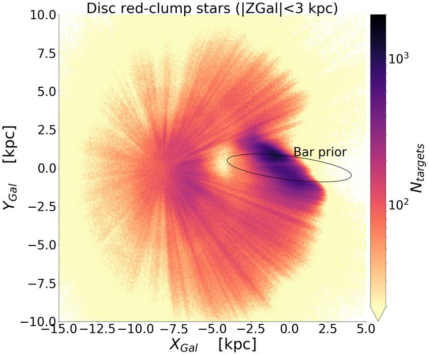
F. Anders et al.: Photo-astrometric distances, extinctions, and astrophysical parameters for Gaia DR2 stars brighter than G = 18

Table 2. Statistics of some of the currently available astro-spectro-photometric distances and extinctions based on Gaia data, in comparison to the
results obtained in this paper. The last three columns refer to the median precision in relative distance, V-band extinction, and effective temperature,
respectively. For the definition of the StarHorse flags we refer to Sect. 3.4.

    Reference                                          Survey(s)                  mag limits        # objects      σd /d        σ AV         σTeff
    Queiroz et al. (2018)                       Gaia DR1 + spectroscopy                                 1.5M       15 %      0.07 mag         –
    Mints & Hekker (2018)                       Gaia DR1 + spectroscopy                                 3.8M       15 %          –            –
    Sanders & Das (2018)                        Gaia DR2 + spectroscopy                                 3.1M       3%        0.01 mag        40 K
    Santiago et al. (in prep.)                  Gaia DR2 + spectroscopy                                   2M       5%        0.07 mag        40 K
    Bailer-Jones et al. (2018)                        Gaia DR2                     G   . 21           1330M        25 %          –            –
    McMillan (2018)                                   Gaia DR2                     G   . 13               7M       6%            –            –
    Andrae et al. (2018)                              Gaia DR2                     G   ≤ 17              80M         –       0.46 mag       324 K
    This work                                   Gaia DR2 + photometry              G   < 18            285M
         StarHorse converged                                                                     265,637,087       28 %      0.25 mag       310 K
         $cal /σcal
                 $ >5                                                                            103,108,516       9%        0.20 mag       265 K
         SH_GAIAFLAG="000"                                                                       232,974,244       26 %      0.24 mag       305 K
         SH_OUTFLAG="00000"                                                                      151,506,183       13 %      0.22 mag       250 K
         both flags                                                                              136,606,128       13 %      0.22 mag       250 K
         All passbands available                                                                  60,520,497       23 %      0.20 mag       270 K
               both flags                                                                         34,447,306       12 %      0.18 mag       220 K
         Gaia DR2+2MASS+AllWISE                                                                   72,754,432       13 %      0.23 mag       255 K
               both flags clean                                                                   52,148,742       9%        0.21 mag       230 K
         Gaia DR2+2MASS                                                                           58,295,744       37 %      0.32 mag       390 K
               both flags clean                                                                   27,616,169       17 %      0.28 mag       300 K
         Gaia DR2 only                                                                            12,486,568       44 %      0.40 mag      1000 K
               both flags clean                                                                    2,003,978       18 %      0.35 mag       390 K
         G ≤ 14                                                                                   16,143,700       5%        0.20 mag       250 K
               both flags clean                                                                   14,432,712       5%        0.20 mag       245 K
         14 < G ≤ 16                                                                              57,368,469       12 %      0.20 mag       250 K
               both flags clean                                                                   49,171,794       12 %      0.20 mag       245 K
         16 < G ≤ 17                                                                              72,801,366       24 %      0.24 mag       300 K
               both flags clean                                                                   43,398,790       16 %      0.23 mag       260 K
         17 < G ≤ 18                                                                             119,323,552       50 %      0.29 mag       380 K
               both flags clean                                                                   29,602,832       14 %      0.24 mag       230 K

millions of brighter stars. Particularly important for our purposes          (G > 16.5), we use the +0.029 mas correction derived by Lin-
are the parallaxes, whose precision varies from < 0.1 mas for                degren et al. (2018) from AllWISE quasars. For intermediate G
G ≤ 17 to ' 0.7 mas for G = 20 (Lindegren et al. 2018). Initial              magnitudes, the parallax correction is linearly interpolated be-
tests showed that reliable StarHorse results (that represent an              tween these two values.
improvement with respect to purely photometric distances) can
be obtained up to G ∼ 18. We therefore downloaded Gaia DR2                       Lindegren et al. (2018); Arenou et al. (2018), and others
data for all stars with measured parallaxes up to that magnitude.            have demonstrated that, similar to the Gaia DR2 parallaxes,
    It is well known that the parallaxes delivered by Gaia DR2               also the parallax uncertainties are prone to moderate systemat-
are not entirely free from systematics (Gaia Collaboration et al.            ics, in the sense that they are typically slightly underestimated.
2018b; Lindegren et al. 2018; Stassun & Torres 2018; Zinn et al.             For this work (see Table 1) we follow a modified version of the
2019; Khan et al. 2019)2 . In particular, Arenou et al. (2018) have          recalibration advertised by Lindegren (2018): in the faint regime
shown that the parallax zero-point is subject to a sub-100µas                (G > 15), the external-to-internal uncertainty ratio exponentially
offset depending on position, and possibly magnitude, parallax,              drops to 1.08, while at the bright end (G < 12) this factor is set
and/or colour. Since our distance inference depends critically on            to 1.2. In the intermediate regime, we again opt for linear in-
the accuracy of the input parallaxes, but the positional depen-              terpolation, a choice that is supported by the data presented by
dence is too complex to calibrate out at the moment, we opted                Lindegren (2018, slide 15).
for the following first-order calibrations detailed in Table 1: in
the bright regime (G < 14), we apply a correction of +0.05 mas                   We note that this re-scaling of the parallax errors takes into
similar to the global offset found by Zinn et al. (2019) and Khan            account the systematic term σ s (which roughly accounts for the
et al. (2019) from asteroseismic and spectroscopic observations              variations of the parallax zero-point over the sky, with magni-
in the Kepler field. It should be noted, however, that Khan et al.           tude, colour etc.; equation 2 in Lindegren 2018) only approxi-
(2019), in agreement with the quasar comparison shown in Are-                mately. By choosing the recalibration detailed in Table 1 we have
nou et al. (2018), find different offsets for the Kepler-2 fields            effectively accounted for σ s in the faint regime. In the bright
C3 and C6, indicating that also in the bright regime the par-                regime, our recalibrated parallax uncertainties are slightly lower
allax zero-point depends on sky position. In the faint regime                than in the Lindegren model (for bright stars our minimum par-
                                                                             allax error is 0.018, below the systematic floor of σ s = 0.021
2
   For a short and comprehensive review, see Lindegren (2018),               proposed by Lindegren). While this will be corrected in future
accessible    at     https://www.cosmos.esa.int/web/gaia/                    runs, we have verified that the results change very little when
dr2-known-issues                                                             correctly including the σ s term.
                                                                                                                         Article number, page 3 of 32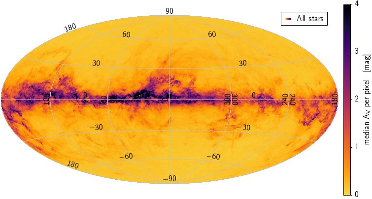
A&A proofs: manuscript no. GDR2_SH

    Apart from the parallaxes, we also make use of the three-
band Gaia DR2 photometry (G, GBP , GRP ). While these are of
an unprecedented precision, several recent works (Weiler 2018;
Maíz Apellániz & Weiler 2018; Casagrande & VandenBerg
2018) have shown by comparison with absolute spectrophotom-
etry that the G band suffers from a magnitude-dependent offset,
and that the nominal passbands need to be slightly corrected.
Therefore, in order to compare the Gaia DR2 G magnitudes to
the synthetic Gaia DR2 photometry from stellar models, we have
applied the G magnitude corrections, as well as the new pass-
band definitions, given by Maíz Apellániz & Weiler (2018).
    Furthermore, we supplement the Gaia data with additional
Pan-STARRS1 grizy (Scolnic et al. 2015), 2MASS JHK s , and
AllWISE W1W2 photometry, using the cross-matches provided
by the Gaia team (Gaia Collaboration et al. 2018b; Marrese et al.
2019). After initial tests, we only used Pan-STARRS1 photom-
etry for stars with magnitudes fainter than G =14 that do not
suffer from saturation problems. For all passbands, missing pho-
tometric uncertainties were substituted by fiducial maximum un-
certainties of 0.3 mag. We also introduced an error floor of 0.04
mag. For Gaia, 2MASS, and AllWISE, we use an uncertainty
floor of 0.03 mag, which can be considered a minimum value
for the accuracy of the synthetic photometry used by our method.
We verified that this choice does not impact our results.

3. StarHorse runs
3.1. The code
The advent of massive multiplex spectroscopic stellar surveys
has led to the development of a growing number of codes that
aim to determine precise distances and extinctions to vast num-
bers of field stars (for example, Breddels et al. 2010; Zwitter
et al. 2010; Burnett & Binney 2010; Binney et al. 2014; Santi-
ago et al. 2016; Wang et al. 2016; Mints & Hekker 2018; Das &
Sanders 2019; Leung & Bovy 2019).
    The StarHorse code (Queiroz et al. 2018) is a Bayesian
parameter estimation code that compares a number of observed         Fig. 1. Dependence of StarHorse posterior distance uncertainty on the
quantities (be it photometric magnitudes, spectroscopically de-      (recalibrated) Gaia DR2 parallax uncertainty. Top: Density plot. Bot-
rived stellar parameters, or parallaxes) to stellar evolutionary     tom: coloured by median log g in each pixel. The grey dashed line indi-
                                                                     cates unity, the red vertical line indicates the approximate value below
models. In a nutshell, it finds the posterior probability over a     which the inverse parallax PDF becomes seriously biased and noisy (see
grid of stellar models, distances, and extinctions, given the set    Bailer-Jones 2015).
of observations plus a number of priors. The priors include the
stellar initial mass function (in our case Chabrier 2003), density
laws for the main components of the Milky Way (thin disc, thick      3.2. Code updates and improvements
disc, bulge, and halo), as well as broad metallicity and age pri-    With respect to Queiroz et al. (2018), a few updates to the
ors for those components. We refer to Queiroz et al. (2018) for      StarHorse code have been carried out. Most importantly, we
more details. In this work we also used a broad top-hat prior on     now take better account of dust extinction when comparing syn-
extinction (−0.3 ≤ AV ≤ 4.0) for stars with low parallax signal-     thetic and observed photometry, an update that was necessary
to-noise ratios ($cal /σcal
                         $ < 5), ensuring the convergence of the     due to the use of the broad-band optical Gaia passbands.
code. This should be kept in mind when interpreting our results          Dust-attenuated synthetic photometry: As explained in
for highly extincted stars in the inner Galaxy. The impact of our    Holtzman et al. (1995); Sirianni et al. (2005), or Girardi et al.
choice of the priors on the results for the inner regions of the     (2008), dust-attenuated photometry of very broad photometric
Galaxy are studied in more detail in Queiroz et al. (in prep.).      passbands (such as the Gaia DR2 ones) should take into account
    The first version of the code was developed by Santiago et al.   that the passband extinction coefficient Ai /AV for a star varies as
(2016) in the context of the RAVE survey (Steinmetz et al. 2006)     a function of its source spectrum Fλ (most importantly its T eff )
and the SDSS-III (Eisenstein et al. 2011) spectroscopic surveys      as well as extinction AV 3 itself:
SEGUE (Yanny et al. 2009) and APOGEE (Majewski et al.                                                     R
2017). In Queiroz et al. (2018) the code was ported to python                    Ai     2.5                  Fλ · T λi dλ
2.7 and made more flexible in the choice of input, priors, etc.                      =      · log10 R                             .
                                                                                 AV     AV            Fλ · T λi · 10−0.4aλ ·AV dλ
With respect to that publication, we have implemented some im-
portant changes that were necessary to apply StarHorse to the         3
                                                                        For simplicity we call our extinction parameter AV , although it refers
huge Gaia DR2 dataset.                                               to A5420Å , as advertised by Schlafly et al. (2016).

Article number, page 4 of 32
F. Anders et al.: Photo-astrometric distances, extinctions, and astrophysical parameters for Gaia DR2 stars brighter than G = 18

Here, T λi is the transmission curve, and aλ is the extinction law.
Therefore, one has to compute the coefficients Ai /AV for each
stellar model and each extinction value considered. In most of
the recent literature concerning stellar distances, this effect is
not taken into account, because for narrow-band and infra-red
passbands, the extinction coefficient is roughly constant. For the
Gaia passbands, however, this is not the case any more (Jordi
et al. 2010). In the new version of StarHorse we therefore use
the Kurucz grid of synthetic stellar spectra (Kurucz 1993)4 to
compute a grid of bolometric corrections as a function of T eff
and AV for each passband, and for our default extinction law
(Schlafly et al. 2016).
    Additional output: While Queiroz et al. (2018) used spec-
troscopically determined stellar parameters as input and there-
fore only reported distances and extinctions (and in the case
of high-resolution spectroscopy also masses and ages; e.g. An-
ders et al. 2018), the absence of spectroscopically determined
effective temperatures, gravities, and metallicities in the case of
Gaia+photometry data led to the decision to also report the pos-
terior values of T eff , log g, and [M/H]. Since the photometric esti-   Fig. 2. Gaia DR2 G magnitude histogram, illustrating the magnitude
mates for log g, [M/H], and stellar mass are of significantly lower      coverage of the different StarHorse sub-samples defined in Table 2.
precision, we regard these as secondary output parameters, in            Inset: zoom into the magnitude range 13 < G < 18 with linear y axis,
contrast to the primary output parameters d, AV , and T eff . The        illustrating the degrading parallax quality around G ∼ 16.5.
secondary parameters were mainly obtained to test the target-
ing strategy of the 4MOST low-resolution disc and bulge survey
(4MIDABLE-LR; Chiappini et al. 2019), and the functionality                  For the case of Gaia DR2 run (i.e. in absence of spectro-
of the 4MOST simulator (4FS; see de Jong et al. 2019). Further-          scopic data), the code took 1 second per star to run on the coarse
more, in addition to the V-band extinction values AV , we also           grid (G > 14, 270M stars), and 20 seconds per star on the fine
provide median extinction values in the Gaia DR2 passbands               grid (G ≤ 14, 16M stars). In total, the computational cost for
G, G BP , and G BP , as well as extinction-corrected absolute mag-       this StarHorse run thus was ∼ 164, 000 CPU hours (19 years
nitude MG0 , and dereddened colour (G BP − G BP )0 .                     on a single CPU). The global statistics for our output results are
                                                                         summarised in Table 2 and discussed in detail in Sect. 4.
    Computational updates: Since Queiroz et al. (2018), the
StarHorse code was migrated python 2.7 to python 3.6
and runs on the newton cluster at the Leibniz-Institut für Astro-        3.4. Input and output flags
physik Potsdam (AIP). Due to several improvements in the data
handling, the runtime was reduced by a factor of 6 as compared           Along with the output of our code (median statistics of the
to the previous version used in Queiroz et al. (2018).                   marginal posterior in distance, extinction, and stellar parame-
                                                                         ters), we provide a set of flags to help the user decide which
                                                                         subset of the data to use for their particular science case. These
3.3. StarHorse setup                                                     flags correspond to the following columns.

We then ran StarHorse code (Santiago et al. 2016; Queiroz
et al. 2018). In this work we used a grid of PARSEC 1.2S stellar         3.4.1. SH_GAIAFLAG
models (Bressan et al. 2012; Chen et al. 2014; Tang et al. 2014)         This flag describes the overall astrometric and photometric qual-
in the 2MASS, Pan-STARRS1, Gaia DR2 rederived (Maíz Apel-                ity of the Gaia DR2 data for each star in a three-digit flag (simi-
lániz & Weiler 2018), and WISE photometric systems available             lar to the Gaia DR2-native priam_flag6 ). Balancing simplicity
on the CMD webpage maintained by L. Girardi5 . For G ≥ 14,               and the recommendations of Lindegren et al. (2018) and Linde-
we use a model grid equally spaced by 0.1 dex in log age as well         gren (2018), we limit this flag to the following three digits:
as in metallicity [M/H]. Due to the higher precision of the Gaia
DR2 parallaxes for G < 14, we used a finer grid with 0.05 dex             1. Renormalised unit weight error flag: Lindegren (2018) re-
spacing in the bright regime.                                                cently showed that instead of following the astrometric qual-
    For computational reasons, depending on the parallax qual-               ity requirements used by Gaia Collaboration et al. (2018b);
ity we used different ways to construct the range of possi-                  Lindegren et al. (2018), and Arenou et al. (2018), similar or
ble distance values: for stars with well-determined parallaxes               better cleaning of spurious Gaia DR2 astrometry can be ob-
($cal /σcal                                                                  tained by requiring a maximum value for the so-called renor-
         $ > 5), we required the distances to lie within {1/($ +
                                                              cal
     cal       cal     cal
4·σ$ ), 1/($ −4·σ$ )}. For stars with less precisely measured                malised unit weight error (ruwe). We therefore defined the
parallaxes, we used their G magnitudes to constrain the distance             first digit as follows:
range for each possible stellar model (for details, see Queiroz                 IF ruwe< 1.4 THEN 0 ELSE 1
et al. 2018).                                                             2. Colour excess factor flag: Evans et al. (2018) and
                                                                             Arenou et al. (2018) recommend the use of the
4
                                                                             phot_bp_rp_excess_factor to flag spurious Gaia
  Provided by the Spanish Virtual Observatory’s Theoretical Spectra
web server (http://svo2.cab.inta-csic.es/theory/newov2/                   6
                                                                           https://gea.esac.esa.int/archive/documentation/GDR2/
index.php).                                                              Data_analysis/chap_cu8par/sec_cu8par_data/ssec_cu8par_
5
  http://stev.oapd.inaf.it/cgi-bin/cmd_3.0                               data_flags.html

                                                                                                                   Article number, page 5 of 32
A&A proofs: manuscript no. GDR2_SH

Fig. 3. corner plot showing the correlations and distributions of StarHorse median primary posterior output values T eff , d, and AV , their corre-
sponding uncertainties, and the G magnitude and parallax precision ($/σ$ ). The grey contours show the distribution of the full sample, while the
red contours show the distribution of all sources with SH_OUTPUTFLAG=="00000" and SH_GAIAFLAG=="000".

   DR2 photometry. We follow their recommendation and                      2MASS, WISE) was used as input for StarHorse. For exam-
   define the second digit as:                                             ple, if photometry in all passbands was available for a star,
     IF GBP − GRP IS NULL THEN 2 ELIF 1.0 + 0.015 · (GBP −                 the SH_PHOTOFLAG entry reads GBPRPgrizyJHKsW1W2. If only
   GRP )2 < phot_bp_rp_excess_factor < 1.3 + 0.060 ·                       Gaia DR2 G and Pan-STARRS1 izy magnitudes were available,
   (GBP − GRP )2 THEN 0 ELSE 1                                             the flag reads Gizy. In addition, in the rare case that no uncer-
3. Variability flag: The third digit equals the Gaia DR2-native            tainty for a particular photometric band was available from the
   phot_variable_flag.                                                     original catalogue and the fiducial uncertainty of 0.3 mag was
                                                                           used instead (see Sect. 2), we added a ’#’ to the correspond-
                                                                           ing passband. For example, if a star has complete Gaia DR2,
3.4.2. SH_PHOTOFLAG                                                        Pan-STARRS1, and WISE photometry, but the r and W2 magni-
The human-readable SH_PHOTOFLAG input flag details which                   tudes come without uncertainties, then the SH_PHOTOFLAG entry
combination of photometric data (Gaia, Pan-STARRS1,                        would be GBPRPgr#izyW1W2#.

Article number, page 6 of 32
F. Anders et al.: Photo-astrometric distances, extinctions, and astrophysical parameters for Gaia DR2 stars brighter than G = 18

Fig. 4. StarHorse posterior Gaia DR2 colour-magnitude diagrams for all converged stars in four magnitude bins, showing the degrading data
quality from G < 14 to G > 17, making the use of the SH_OUTFLAG mandatory especially the faint regime (see Fig. 5).

3.4.3. SH_PARALLAXFLAG                                                   3.4.4. SH_OUTFLAG
                                                                         The StarHorse output flag, similar to SH_GAIAFLAG, consists
                                                                         of several digits that inform about the fidelity of the StarHorse
                                                                         output parameters.
The SH_PARALLAXFLAG input flag informs about the precision of
the Gaia DR2 parallaxes (accounting for zero-point shift and un-          1. Main StarHorse reliability flag: If this digit equals to 1,
certainty corrections; see Table 1). For $cal /σcal
                                                $ > 5 (parallaxes
                                                                             then the star has a very broad distance PDF:
better than 20%), the flag reads gtr5, else leq5. As explained in            ( IF      0.5 · (dist84 − dist16)/dist50                       <
Sec. 3.3, this has consequences for the construction of the poste-             0.35                        logg50 > 4.1
                                                                                                                             THEN 0 ELSE
rior PDF in the StarHorse code: if the parallax is precise, then               1.0347 − 0.167 · logg50 logg50 ≤ 4.1
the range of possible distances is computed directly from the                1
parallax itself (allowing for 4σ deviations). On the other hand,             We justify this definition, a cut in the posterior log g vs.
if only uncertain parallaxes are available, the range of possible            distance plane, in Appendix A. The essence of this defini-
distance moduli is constructed based on the measured G mag-                  tion is that median statistics of the posterior parameters for
nitude. We verified that this choice does not produce different              stars where this digit equals to 1 should be treated with ut-
results for stars near the decision boundary (the rupture in Fig.            most care, as their combination often yields unphysical re-
1 does not occur at the decision boundary $cal /σcal$ = 5, but at            sults. For instance, some stars fall in places of the extinction-
' 1./0.22 ' 4.55, which is where the standard deviation of the               corrected CMD that is inconsistent with any stellar model
inverse parallax PDF increases sharply; see Bailer-Jones 2015,               (due to complex multi-modal PDFs; see Appendix B), mean-
Sect. 4.1).                                                                  ing that their median posterior absolute magnitude, distance,
                                                                                                                   Article number, page 7 of 32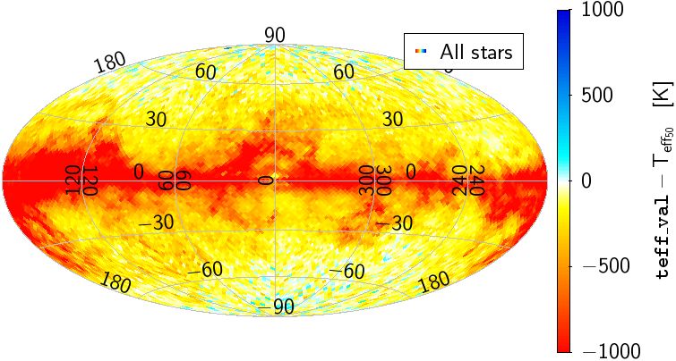
A&A proofs: manuscript no. GDR2_SH

Fig. 5. StarHorse Gaia DR2 colour-magnitude diagrams, colour-coded as in Table 2. Top left: CMD resulting from all stars for which the
code converged (266 million stars). Top right: emphasising sources with (recalibrated) parallaxes better than 20% (103 million stars). Bottom
row: emphasising the effect of cleaning the results by means of the StarHorse flags (see discussion in Sec. 3.4) Bottom left: cleaning only by
SH_OUTFLAG (152 million stars). Bottom right: cleaning by both SH_OUTFLAG and SH_GAIAFLAG (137 million stars).

   and extinction should not be used together (see for instance             dSph), StarHorse delivers very large posterior distances,
   the unphysical ’nose’ feature between the main sequence and              many of which are likely affected by significant biases due
   the red-giant branch in Fig. 4, bottom right panel). We veri-            to the dominance of the Galactic prior used to infer them: IF
   fied that this effect only occurs for faint stars with very uncer-       dist50 < 20 THEN 0 ELIF dist50 < 30 THEN 1 ELSE 2
   tain parallaxes (σcal$ /$
                             cal
                                 & 22%) - which is when the PDF          3. Unreliable extinction flag: Significantly negative extinctions,
   of inverse parallax becomes very noisy and biased (see Fig. 1            or AV values close to the prior boundary at AV = 4 should be
   and Bailer-Jones 2015; Astraatmadja & Bailer-Jones 2016b;                treated with care: IF (AV95 > 0 AND AV95 < 3.9 THEN 0
   Luri et al. 2018). This results in a poor discrimination be-             ELIF AV95 < 0 THEN 1 ELIF AV84 < 3.9 THEN 2 ELSE 3
   tween dwarfs and giants for these typically faint (G & 16.5;          4. Large AV uncertainty flag: Very large extinction uncertain-
   see Fig. 2) stars. Although their median effective tempera-              ties point to either incomplete or very uncertain input data:
   tures and extinctions may still be useful, their median 1D dis-          IF 0.5 · (AV84 − AV16) < 1 THEN 0 ELSE 1
   tances and other parameters should not be used. We discuss            5. Very small uncertainty flag: Very small posterior uncer-
   the issue in more detail in Appendix A. In future StarHorse              tainties are most likely underestimated and indicate poor
   runs we will resort to a more sophisticated treatment of mul-            StarHorse convergence (either due to inconsistent in-
   timodal posterior PDFs.                                                  put data or too coarse model grid size). These results
2. Large distance flag: For some stars (especially extragalac-              should therefore also be used with care. The definition
   tic objects that are still bright enough to be in Gaia DR2,              is as follows: IF 0.5 ∗ (dist84 − dist16)/dist50 <
   such as stars in the Magellanic Clouds or the Sagittarius                0.001 OR 0.5 ∗ (av84 − av16) < 0.01 OR 0.5 ∗
Article number, page 8 of 32
F. Anders et al.: Photo-astrometric distances, extinctions, and astrophysical parameters for Gaia DR2 stars brighter than G = 18
Fig. 6. StarHorse-derived Kiel diagrams. Top left: overall density plot before applying quality cuts. Top middle: colour-coded by median distance.
Top right: colour-coded by median distance uncertainty. Lower left: flag-cleaned sample coloured by density. Lower middle: colour-coded by
median AV . Lower right: colour-coded by median AV uncertainty.
(teff84 − teff16) < 20. OR 0.5 ∗ (logg84 − logg16) < dataset). In particular, the table informs about sample sizes, mag-
0.01 OR 0.5 ∗ (met84 − met16) < 0.01 OR 0.5 ∗ nitude ranges, and the typical precision in the primary output pa-
(mass84 − mass16)/mass50 < 0.01 THEN 1 ELSE 0. rameters d, AV , and T eff . In this table, we also define some use-
ful sub-samples of the Gaia DR2 StarHorse data (identified by
colour in some of the subsequent plots) that are used throughout
this paper. These are:
3.5. Data access
1. stars with (recalibrated) parallaxes more precise than 20%
StarHorse delivered distances and extinctions for 265,637,087 (blue colour; 39% of the converged stars),
objects, of which 151,506,183 pass the post-calculo quality flags 2. stars with SH_GAIAFLAG equal to "000" (cyan colour; 88%
included in SH_OUTFLAG, and 136,606,128 stars pass both the of the converged stars),
SH_OUTFLAG as well as the SH_GAIAFLAG that includes the re- 3. stars with SH_OUTFLAG equal to "00000" (orange colour;
cent recommendations of Lindegren et al. (2018). For clarity, all 57% of the converged stars),
our calibration choices are listed in Table 1. The main statistics 4. stars with SH_OUTFLAG equal to "00000" and SH_GAIAFLAG
are summarised in Table 2. Our results, together with documen- equal to "000" (red colour; 52% of the converged stars).
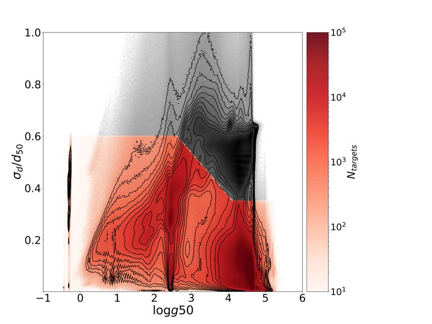
tation, can be queried via the AIP Gaia archive at gaia.aip.de. The G magnitude distribution for each of these sub-samples is
Example queries can be found in Appendix D. In addition, shown in Fig. 2. In this paper, we will mainly concentrate on the
the output files are available for download in HDF5 format at "both-flags"-cleaned sample.
data.aip.de. The digital object identifier for this dataset is Figure 3 presents the output of the StarHorse code for the
doi:10.17876/gaia/dr.2/51. Gaia DR2 sample in one plot. The figure displays the distribu-
tions and correlations of the median StarHorse primary out-
put parameters T eff , d, and AV , and their respective uncertainties,
4. StarHorse Gaia DR2 results as well as G magnitude and parallax signal-to-noise ratio. The
4.1. Summary grey contours in this plot refer to all converged stars, whereas
the red contours emphasise the results for the stars with both
Table 2 summarises the results of the present StarHorse run for SH_GAIAFLAG and SH_OUTFLAG equal to "00000". For a plot in-
Gaia DR2 and puts them in context with previous results avail- cluding also the secondary output parameters log g, [M/H], and
able from the literature (three references for distances and ex- M∗ , we refer to Fig. B.1.
tinctions for Gaia stars observed by spectroscopic surveys, as The panels in the diagonal row of Fig. 3 provide the one-
well as the two only studies that attempted to determine dis- dimensional distributions in G magnitude, parallax signal-to-
tances and extinctions, respectively, for the whole Gaia DR2 noise, the median output parameters, and the distributions of
Article number, page 9 of 32A&A proofs: manuscript no. GDR2_SH
Fig. 7. Left: StarHorse density maps for the SH_GAIAFLAG== ”000”,SH_OUTFLAG= ”00000” sample in Galactocentric co-ordinates. Top left:
XY map. Top right: YZ map. Bottom left: XZ map. Bottom right: RZ map. These density maps demonstrate that Gaia DR2 already allows to probe
stellar populations in the Galactic bulge and beyond.
the corresponding uncertainties (in logarithmic scaling) as area- 4.2. Extinction-cleaned CMDs
normalised histograms. Each of the panels also illustrates the ef-
fect of applying the recommended flags: the red uncertainty dis- As a first sanity check, in Fig. 4 we present StarHorse-derived
tributions are typically confined to smaller values than the faint Gaia DR2 colour-magnitude diagrams (CMDs) for the full con-
grey ones. verged sample (i.e. excluding mostly white dwarfs and galax-
ies) in four magnitude bins. Focussing first on the top left panel
(G < 14), we note very well-defined features of stellar evolution
the CMD: a thin main sequence (broadening in the very blue and
The off-diagonal plots of Fig. 3 show the correlations be- very red regimes), a well-populated sub-giant branch, as well as
tween the output parameters. We observe complex structures in a very thin red clump, the red giant branch, and the asymptotic
many of these panels, most of which are due to physical corre- giant branch. We also notice more subtle features such as the
lations stemming from stellar evolution or selection effects. For red-giant bump or the secondary red clump.
example, the strong bimodality between giants and dwarfs in the As we move to fainter magnitude bins, the number of ob-
log g vs. T eff diagram (see third column, second panel from top jects grows, but also the typical uncertainty in the main input pa-
in Fig. B.1) is reflected in many of the panels, most notably the rameter parallax, resulting in a gradual broadening of the sharp
distance distribution (fourth column). In addition, we note that stellar-evolution features observed in the top left panel of Fig.
some of the complex structure disappears when the flag cleaning 4. In the lower left panel, for example, we begin to note some
is applied to the data. Different behaviour of the red and grey additional features that are not directly related to stellar evolu-
distributions in some panels should warn the user about poten- tion. For example, the almost vertical arm at (BP − RP)0 below
tially spurious correlations that may appear when using the full the main sequence is related to problematic astrometry (large
StarHorse sample. ruwe values). Furthermore, the discrete stripes in the red main
Article number, page 10 of 32F. Anders et al.: Photo-astrometric distances, extinctions, and astrophysical parameters for Gaia DR2 stars brighter than G = 18
Fig. 8. XY density map, selecting only flag-cleaned red-clump stars less
than 3 kpc away from the Galactic midplane. 10,807,155 stars are con-
tained in this figure. The ellipse indicates the shape of the bar/bulge
density prior adopted for this work (Robin et al. 2012 model B; see
Queiroz et al. 2018 for details).
sequence are related to the finite mass, age, and metallicity res-
olution of our stellar model grid used. Some other unphysical
structures, such as the nose between the main sequence and the
giant branch, are induced by poor convergence of StarHorse
(see Sect. 3.4.4). The higher relative number of giant stars in the
fainter magnitude bins with respect to the G < 14 sample is an
effect of stellar population sampling.
Figure 5 shows another collection of StarHorse CMDs,
now highlighting the sub-samples defined in Table 2. As dis-
cussed in Sect. 3.4.4, the full StarHorse sample occupies a
larger volume in the CMD, including an unphysical region in-
between the main sequence and the red-giant branch that is due
to stars with poorly determined parallaxes. These stars disappear Fig. 9. Top panel: Median proper motion in Galactic longitude, µl , LSR,
when applying the SH_OUTFLAG (orange dots in lower middle per pixel in Cartesian Galactic co-ordinates, for the disc RC sample
panel), and a further cleaning using the SH_GAIAFLAG results in shown in Fig. 8. Overplotted are the highest density contours from Fig.
a nice physical CMD for 129 million stars (lower right panel of 8, highlighting the overdensity of the Galactic bar. The arrow highlights
the direction of the solar motion used to correct the proper motion map.
Fig. 5).
The large µl values close to the solar position point to a residual correc-
Comparing the upper right and lower right panel of Fig. tion that may be necessary. Bottom panel: The same proper motion map
5, we see that the number of red giants in the latter is much for the disc red-giant sample used in Romero-Gómez et al. (2019).
higher, leading to a slight broadening of the RC locus and a sub-
stantially higher number of AGB stars. This is due to the fact
that StarHorse is able to determine still surprisingly precise 4.4. Stellar density maps and the emergence of the Galactic
(∼ 30%) photo-astrometric distances for giants with poor paral- bar
lax measurements.
Figure 7 presents four projections of the stellar density dis-
tribution in Galactocentric co-ordinates for the flag-cleaned
4.3. Kiel diagrams sample. The solar position (in kpc) is at (XGal , YGal , ZGal ) =
(8.2, 0, 0.025). The figure emphasises the loss of stars near the
Figure 6 shows Kiel diagrams (log g vs. T eff ) using the median Galactic midplane towards the inner Galaxy, which is due to both
posterior StarHorse results, for the full sample of converged the high dust extinction affecting the Gaia selection function,
stars and for the flag-cleaned sample defined in Table 2. The and the low number of stars that pass the flag quality criteria in
middle column of that figure show the the median distance and these regions. Several conclusions can be drawn from Fig. 7, as
median AV extinction in each pixel of the Kiel diagram, respec- we describe next.
tively. The right column show their respective uncertainties in As pointed outed by Bailer-Jones (2015); Luri et al. (2018),
each pixel. The complex dependence of the uncertainties on the for example, the naive 1/$ estimator provides biased distances,
stellar parameters reflects the abrupt decrease in precision below especially in the case of low parallax precision, extending the
$cal /σcal
$ = 5 seen in Fig. 1. observed volume to unplausibly large distances. On the other
Article number, page 11 of 32A&A proofs: manuscript no. GDR2_SH
Fig. 10. All-sky median StarHorse extinction map using all converged stars up to G < 18.
hand, the exponentially decreasing density prior recently used The lower right panel of Fig. 7 shows the density map in
by Bailer-Jones et al. (2018) is more apt for main-sequence stars Galactocentric cylindrical co-ordinates RGal vs ZGal . Especially
and tends to underestimate the distances to distant luminous gi- in this panel we note two overdensities in the direction of the
ant stars. The StarHorse results for those stars, taking into ac- Magellanic Clouds. These are mostly composed of stars belong-
count photometric information as well as more complex priors, ing to the Clouds that have been forced to smaller distances by
show for the first time that Gaia DR2 already allows us to probe our Milky Way prior (which does not contain any extragalactic
stellar populations in the bulge and beyond. A detailed compari- stellar population, only a smooth halo with a power-law den-
son with Bailer-Jones et al. (2018) is presented in Section 6.1. sity). The results for these stars have not been excluded from our
The clearest novel feature of the StarHorse density map analysis, but should be used with caution. The same is true for
shown in Fig. 7 is the presence of a stellar overdensity coincid- other nearby galaxies with resolved stellar populations, such as
ing with the expected position of the Galactic bar, inclined by the Sagittarius dSph, Fornax, etc.
about 40 degrees with respect to the solar azimuth, and with
a semi-major axis of about 4 kpc. This almost direct detec- 4.5. Kinematic maps
tion of the Galactic bar is confirmed with StarHorse distances
for APOGEE stars and discussed in detail in a separate paper Several studies have already used our distances for the Gaia DR2
(Queiroz et al., in prep.). The significance of the result lies in the sub-sample of stars with radial velocity measurements (Katz
fact that although we are using a prior for the Galactic bulge- et al. 2019) in kinematic analyses of the Galactic disc. Quillen
bar (Robin et al. 2012), its shape and inclination angle are quite et al. (2018) used our results to study the arches and ridges in ve-
different from our bar prior (see Fig. 8), even when invoking an locity space found by Gaia Collaboration et al. (2018d); Antoja
interplay with possible observational biases. et al. (2018) and Kawata et al. (2018), attributing some of them
The presence of the Galactic bar in the Gaia DR2 data is even to stellar orbit crossings with spiral arms. Monari et al. (2018)
more prominent when we focus only on the red-clump stars. Fig. used our distances to counter-rotating stars in the Galactic halo
8 shows the resulting density map when selecting flag-cleaned to measure the escape speed curve and the mass of the Milky
RC stars close to the Galactic plane (|ZGal | < 3 kpc) from the Way. Recently, Carrillo et al. (2019) used StarHorse distances
StarHorse Kiel diagram (4500 K< teff50 < 5000 K, 2.35 < together with Gaia DR2 positions, proper motions, and line-of-
logg50 < 2.55, −0.6 < met50 < 0.4). The density contrast of sight velocities, to study the 3D velocity distribution in the Milky
the RC bar with respect to the RC population in front of the bar Way disc. They confirmed the bulk vertical motions see in ear-
amounts to almost 50. This could in fact be a physical feature of lier data, consistent with a combination of breathing and bending
the Galactic disc: the RC is a tracer of the young-to-intermediate modes, and identified a strong radial VR gradient in the Galactic
age population (∼ 1 − 4 Gyr; e.g. Girardi 2016), and the star- inner disc, transitioning smoothly from 15 km/s/kpc at Galac-
formation history in the inner disc outside the bar region is still tic azimuth ΦGal ∼ 50 deg to -15 km/s/kpc at Galactic azimuth
poorly constrained. It is more likely, however, that the observed ΦGal ∼ −50 deg. Our StarHorse results were essential for this
shape of the bar (and especially the density drop in front of it) in type of work, since they enabled the authors to probe much far-
Fig. 8 is a combined effect of the Gaia DR2 selection function, ther heliocentric distances.
the stellar density profile of the inner disc, our adopted bulge To further illustrate the accuracy of our distances for distant
prior, and the quality flag cuts used to produce Fig. 8. At the red-giant stars, in Fig. 9 we show a proper-motion map of the
present stage, we therefore caution the reader not to take the star disc red-clump sample used in Fig. 8 and Sect. 4.4. Both pan-
count numbers in this map at face value, and refer to Queiroz et els of Fig. 9 show proper motion in Galactic longitude corrected
al. (in prep.) for a more in-depth discussion. for the solar motion, µl,LSR , as a function of Galactic position.
Article number, page 12 of 32F. Anders et al.: Photo-astrometric distances, extinctions, and astrophysical parameters for Gaia DR2 stars brighter than G = 18
Fig. 11. Distance-binned extinction maps for the Orion region, using the same dimensions as Zari et al. (2017). The number of stars contained in
each subplot is 228,808, 282,009, 297,862, and 246,266, respectively.
The top panel shows the StarHorse red-clump stars, while the The prominent symmetric arc features around the solar posi-
bottom panel shows the red-giant sample studied by Romero- tion towards the outer and inner disc are produced by the Galac-
Gómez et al. (2019). For comparability, we assume the same tic rotation curve, and follow the overall expected trends (see
values for the solar motion (U = 11.1 km/s, V = 12.24 km/s; e.g. Fig. 3 in Brunetti & Pfenniger 2010 for a prediction of the
Schönrich et al. 2010) and the distance to the Galactic Centre µl map for an axisymmetric disc). It is interesting to see that the
(8.34 kpc; Reid et al. 2014) as in Romero-Gómez et al. (2019), proper motion contours in the inner disc coincide with the angle
although the residual small-scale dipole variations close to the of the Galactic bar (defined by stellar density). Qualitatively this
solar position suggest that the solar motion correction may have coherent motion seen in the region of the bar agrees with earlier
to be slightly revised. predictions by Brunetti & Pfenniger (2010, their Fig. 8) and the
disc red-clump test particle simulations of Romero-Gómez et al.
The study of Romero-Gómez et al. (2019) concerned the
(2015).
morphology and kinematics of the Galactic warp, so it mainly
focussed on the motions perpendicular to the Galactic disc, µb . A more quantitative comparison to kinematic Galactic mod-
Here we show that the µl map of the RGB sample in the bottom els including effects of the Galactic bar is left to future studies.
panel of Fig. 8 compares quite well to our red-clump sample
shown in the top panel. Since here we are more interested in the 4.6. Extinction maps
possible kinematic effects of the Galactic bar, we can now study
the bulk motions in the Galactic plane out to larger distances Figures 10 and 11 show StarHorse-derived two-dimensional
from the Sun, using a cleaner sample of RC stars. We highlight (2D) median extinction maps. Figure 10 shows the all-sky AV
several dynamical features present in this sample. map in Aitoff projection. The overall appearance of this figure
Article number, page 13 of 32A&A proofs: manuscript no. GDR2_SH
Fig. 12. StarHorse posterior parameter precision as a function of Gaia DR2 G magnitude, showing the median trends for different subsets of the
data, and highlighting the improvement in precision when including additional photometry. Top row: Primary output parameter precision (from
left to right: σd /d, σAV , σTeff ). Bottom row: Secondary output parameter precision (from left to right: σlog g , σ[M/H] , σ M∗ /M∗ ).
compares very well to the expected 2D extinction map (e.g. An- output parameters) is of course not the magnitude itself, but the
drae et al. 2018, Fig. 21; Lallement et al. 2018, Fig. 6). parallax signal-to-noise ratio (e.g. Bailer-Jones et al. 2018, see
In Fig. 11, we show median extinction maps in four dis- also Fig. 1). The complex correlations between the output pa-
tance bins between 300 and 1500 pc, for the Orion region. The rameters and their uncertainties are shown in Fig. 3 for the pri-
four panels show how with increasing distance extinction from mary output parameters. For a global picture of the parameter
molecular clouds gradually fills the Galactic plane. In principle, and uncertainty trends including the secondary output parame-
our results can thus be used to construct 3D extinction maps (e.g. ters, we refer to Fig. B.1. For the sake of brevity, however, here
Schlafly & Finkbeiner 2011; Green et al. 2015) and infer the we focus our discussion mainly on the median uncertainty trends
three-dimensional dust distribution in the extended solar vicin- with G magnitude (which is correlated with $/σ$ ) shown in
ity (e.g. Capitanio et al. 2017; Rezaei Kh. et al. 2018; Lallement Fig. 12.
et al. 2019; Zucker et al. 2019). The distance precision plot (top left panel of Fig. 12) de-
serves some further discussion. To begin with, in the bright
5. Precision and accuracy regime (G DR2 < 14, including the radial-velocity sub-sample
of 7 · 106 stars), the vast majority of stars have uncertainties of
5.1. Overall precision 8% or less in distance, as expected from the exquisite parallax
Figure 12 shows the median relative uncertainties in the quality of Gaia DR2 (Lindegren et al. 2018; Arenou et al. 2018).
StarHorse output parameters as a function of Gaia DR2 G Focussing on the orange and blue lines of this plot, it may be sur-
magnitudes. In all panels, we again show the results for all prising that the addition of 2MASS magnitudes to the input data
converged stars (in black, as before), and for the flag-cleaned seems to worsen the distance precision. In fact, the most precise
sample (in red, as before). The other coloured lines shown distances for stars with G < 12.5 are obtained when only using
in Fig. 12 demonstrate the precision improvement obtained Gaia DR2 data. This observation points to a tension between the
by adding more photometric data to the Gaia DR2 data. The 2MASS and the Gaia DR2 data: The range of acceptable dis-
blue curves denote the running median uncertainty for stars tances for these stars is precisely determined by their measured
with only Gaia DR2 photometry, while the other coloured parallax (we assume the parallax offset to be fixed and only a
lines refer to stars for which other data are available (as in- function of magnitude; see Table 1); so that the three Gaia DR2
dicated in the legend in the middle panels). The green curve passbands alone already constrain the space of possible stellar
stands for the stars with complete photometric information parameters and extinctions. The three 2MASS magnitudes alone
(SH_PHOTOFLAG=="GBPRPgrizyJHKsW1W2"). also constrain effective temperature and extinction, so if these
Uncertainties in most quantities increase with G, as ex- two independent constraints are in tension with each other (most
pected, due to the increasing uncertainties in the astrometry and likely due to an underestimated - systematic - parallax uncer-
photometry (we note the logarithmic y-axis in all panels of Fig. tainty), the uncertainty on the output distance increases.
12, except the top middle). The fundamental determinant for the For a similar, but not identical reason, the addi-
distance precision (as well as for most of the other StarHorse tion of Pan-STARRS1 magnitudes to the set of Gaia
Article number, page 14 of 32F. Anders et al.: Photo-astrometric distances, extinctions, and astrophysical parameters for Gaia DR2 stars brighter than G = 18
Fig. 13. Median uncertainty distributions σd /d50 (left) σAV (middle), and σTeff (right) as a function of position in Galactic co-ordinates. Top row:
for all converged stars. Bottom row: for the SH_GAIAFLAG= ”000” & SH_OUTFLAG= ”00000” sample.
DR2+2MASS+AllWISE photometry does not improve the dis- secondary output parameters log g, [M/H], and stellar mass M∗ .
tance precision, but has a slight effect in the opposite direction For the latter we also note an (at first sight puzzling) decreasing
(compare magenta and green lines in Fig. 12). We suggest that trend of the overall median uncertainty (black line in bottom
this points to an inconsistency between the Gaia DR2 photome- right panel of Fig. 12) up to G ∼ 14, which is an effect of the
try with the Pan-STARRS1 one. Since the Gaia DR2 photometry different sampling of stellar populations at different magnitudes.
is of unprecendented precision, and the transmission curves and
zeropoints are well-characterised (at least for not too red stars, Figure 13 shows the median uncertainties in the primary out-
GBP − GBP . 1.5) by Maíz Apellániz & Weiler (2018), we tenta- put parameters d, AV , and T eff for stars in the Galactic disc as a
tively suggest that this indicates a need for additional corrections function of their position. The top row shows the precision in
of the PS1 zeropoints. However, we decided to keep the PS1 pho- each pixel in the X vs. Y plane for all converged stars, while the
tometry as input where possible, since the five optical passbands bottom row shows the corresponding results for the flag-cleaned
considerably help in increasing the precision of extinction and sample.
metallicity (see top middle and bottom middle panel of Fig. 12). The top left panel demonstrates the sharp transition into the
The wiggle in the median uncertainty at G ∼ 13 is due to low-signal-to-noise parallax regime at heliocentric distances of
the decrease in parallax uncertainty at that magnitude transition ∼ 2.5 kpc (the Gaia DR2 "parallax sphere"). In the bottom left
(Lindegren et al. 2018). The sharp increase in median distance panel, this effect is much less severe, because of many distant
uncertainty at G ' 16.5 is due to the transition into the low- giant stars passing the quality criteria of the StarHorse flags.
signal-to-noise parallax regime. In particular, the distance un- Even in the Galactic bar region, the typical uncertainties for the
certainties are much larger for faint main-sequence stars, which flag-cleaned sample only amount to ∼ 30%.
fill the locus of G DR2 > 16.5 and σd /d > 0.5, whereas the (pre- The middle panels of Fig. 13 especially highlight the de-
dominantly photometric) distances to distant red giants remain crease in AV precision in the quarter of the sky for which no
more precise (see Fig. 1). Pan-STARRS1 photometry is available. We also note that out-
The flag-cleaned results, by construction, yield much more side the solar vicinity our extinction estimates are more precise
precise results also in the faint regime. The drop in median un- in regions dominated by giant stars, resulting in a ring around the
certainty for those stars is due to the distance precision cut em- Sun for which the uncertainties are higher. The same is true for
bedded in the definition of the SH_OUTFLAG (see Appendix A). the effective temperatures (right panels), because the two poste-
For the precision in AV extinction (top middle panel of Fig. rior quantities are correlated (see Appendix B for a short discus-
12), we note a flat trend as a function of G, with the uncertainty sion of the correlations of correlations in the estimated parame-
increasing significantly only in the regime where parallaxes and ters).
distances become much more uncertain (G ' 16.5). We also note
the expected increase in precision when including more photo-
5.2. Accuracy: Comparison to asteroseismology
metric passbands (see also Table 2).
Similar observations hold for the median uncertainties It is difficult to find true benchmark tests for the distance, extinc-
in effective temperature as well as the uncertainties in the tion, and stellar parameter scales of large surveys that are not
Article number, page 15 of 32You can also read