Uncertainty in temperature response of current consumption-based emissions estimates
←
→
Page content transcription
If your browser does not render page correctly, please read the page content below
Earth Syst. Dynam., 6, 287–309, 2015
www.earth-syst-dynam.net/6/287/2015/
doi:10.5194/esd-6-287-2015
© Author(s) 2015. CC Attribution 3.0 License.

                 Uncertainty in temperature response of current
                   consumption-based emissions estimates
                                       J. Karstensen, G. P. Peters, and R. M. Andrew
         Center for International Climate and Environmental Research – Oslo (CICERO), P.O. Box 1129, Blindern,
                                                    0318 Oslo, Norway
                             Correspondence to: J. Karstensen (jonas.karstensen@cicero.oslo.no)
                        Received: 17 July 2014 – Published in Earth Syst. Dynam. Discuss.: 9 September 2014
                             Revised: 8 April 2015 – Accepted: 13 April 2015 – Published: 27 May 2015

       Abstract. Several studies have connected emissions of greenhouse gases to economic and trade data to quantify
       the causal chain from consumption to emissions and climate change. These studies usually combine data and
       models originating from different sources, making it difficult to estimate uncertainties along the entire causal
       chain. We estimate uncertainties in economic data, multi-pollutant emission statistics, and metric parameters,
       and use Monte Carlo analysis to quantify contributions to uncertainty and to determine how uncertainty prop-
       agates to estimates of global temperature change from regional and sectoral territorial- and consumption-based
       emissions for the year 2007. We find that the uncertainties are sensitive to the emission allocations, mix of pol-
       lutants included, the metric and its time horizon, and the level of aggregation of the results. Uncertainties in the
       final results are largely dominated by the climate sensitivity and the parameters associated with the warming
       effects of CO2 . Based on our assumptions, which exclude correlations in the economic data, the uncertainty
       in the economic data appears to have a relatively small impact on uncertainty at the national level in compari-
       son to emissions and metric uncertainty. Much higher uncertainties are found at the sectoral level. Our results
       suggest that consumption-based national emissions are not significantly more uncertain than the corresponding
       production-based emissions since the largest uncertainties are due to metric and emissions which affect both
       perspectives equally. The two perspectives exhibit different sectoral uncertainties, due to changes of pollutant
       compositions. We find global sectoral consumption uncertainties in the range of ±10 to ±27 % using the Global
       Temperature Potential with a 50-year time horizon, with metric uncertainties dominating. National-level uncer-
       tainties are similar in both perspectives due to the dominance of CO2 over other pollutants. The consumption
       emissions of the top 10 emitting regions have a broad uncertainty range of ±9 to ±25 %, with metric and emis-
       sion uncertainties contributing similarly. The absolute global temperature potential (AGTP) with a 50-year time
       horizon has much higher uncertainties, with considerable uncertainty overlap for regions and sectors, indicating
       that the ranking of countries is uncertain.

1   Introduction                                                    has been shown that territorial emissions have decreased in
                                                                    most developed countries since 1990, but consumption-based
Many studies have shown that national greenhouse gas                emissions have increased (Peters et al., 2011c). This indicates
(GHG) emission accounts can be viewed from either a                 that growth in consumption and international trade may un-
production (territorial) or consumption perspective (Davis          dermine the effectiveness of climate policies that only limit
and Caldeira, 2010; Hertwich and Peters, 2009; Wiedmann,            emissions in a subset of countries, such as in the Kyoto Pro-
2009; Peters and Hertwich, 2008). While the production view         tocol (Wiebe et al., 2012; Kanemoto et al., 2013).
only looks at territorial emissions, the consumption view in-          The concept of consumption-based emissions estimates
cludes emissions from the production of imported products           can therefore be used to extend the cause–effect chain from
and excludes emissions from the production of exports. It           consumption, to production, to emissions, and ultimately to

Published by Copernicus Publications on behalf of the European Geosciences Union.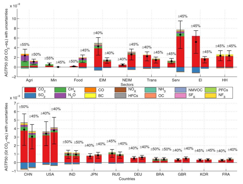
288                                                          J. Karstensen et al.: Current consumption-based emissions estimates

                     5
                                                                         relevant species. In addition, there are almost no estimates of
                         Consumption
                     4

                     3

                                                                         uncertainty at the sector level. Many aspects of uncertainty
                     2

                     1

                     0

                                                                         have been investigated in the climate system (Skeie et al.,
                                         Economic data
                                                                         2013; Prather et al., 2012; Myhre et al., 2013b), but there
                                                                         is little literature on the uncertainties in emissions metrics
                         Production                                      (Olivié and Peters, 2013; Shine et al., 2007; Reisinger et al.,
                                         Emissions data
                                                                         2010). We are not aware of any studies that have estimated
                                                                         the uncertainty introduced by each model and data set (e.g.,
                 5

                                                                         metric and IO uncertainties), or how uncertainty propagates
                         Emissions
                 4

                 3

                 2

                                                                         when estimating climate change from consumption as a so-
                 1

                 0

                                              Metrics                    cioeconomic driver.
                                                                            We extend the uncertainty analyses done by Prather et
             5

                                                                         al. (2009), Höhne et al. (2010), and den Elzen et al. (2005)
                         Temperature change
             4

             3

             2

                                                                         by including consumption-based emissions for a single year
             1

             0

                                                                         and using a temperature-based emission metric, which is ar-
Figure 1. Flow chart of activities (bold boxes) and the data sets that
                                                                         guably a more policy-relevant method of weighting emis-
determine transitions between them (dashed boxes).
                                                                         sions. We use Monte Carlo analysis and draw on previous
                                                                         studies of uncertainties to perturb and highlight the different
                                                                         contributors: economic data, emissions, and metric parame-
global warming (Fig. 1). This is an important complement                 ters, and then compare our results with the previous studies.
to the established territorial (Kyoto Protocol) viewpoint, par-
ticularly in that it links more directly to consumption as a
key driver of emissions. More recent studies have broadened              2   Methods
this concept to look at further consequences of increased
global demand for traded products, such as deforestation                 We consider the propagation of uncertainty from the point
(Karstensen et al., 2013), biodiversity loss (Lenzen et al.,             of consumption of goods and services (products), to the pro-
2012b), dependency on traded fossil fuels (Andrew et al.,                duction of products where emissions occur, to the climate im-
2013), land-use change (Weinzettel et al., 2013), and water              pacts caused by those emissions (Fig. 1). This can be thought
footprints (Hoekstra and Mekonnen, 2012).                                of as a causal chain where consumption is assumed to be the
   In the estimation of consumption-based emissions ac-                  primary driver, in turn driving production, which in turn leads
counts, various data sets and models are combined in the cal-            to emissions, which then lead to temperature change. These
culations, and thus uncertainties and errors may arise in a              components of the cause–effect chain are linked by calcu-
number of data sets and models: emission data, metric data,              lation methodologies, each requiring parameterization, and
economic data, etc. There are also uncertainties in assump-              we break the analysis into those three components: economic
tions and study design that can be more difficult to explicitly          data, emission statistics, and emission metrics. We estimate
quantify, including which metric and time horizon to use for             the uncertainty for each of the components individually and
comparing pollutants, and how economic data for one spe-                 finally connect the components to determine how uncertainty
cific year can be relevant to other years.                               propagates through the cause–effect chain.
   The uncertainty of many aspects of the cause–effect                      To determine the temperature response to a given level of
chain have been investigated previously (Höhne et al., 2010;             consumption, we first map emission statistics for most im-
Prather et al., 2012), but the link to consumption has not               portant pollutants to producing regions and sectors (Euro-
been made. There is a growing literature on the uncertainty              pean Commission, 2011). Emissions are then converted into
in input–output (IO; economic) models used to estimate                   global temperature change using an emission metric (Aa-
consumption-based emissions (Wilting, 2012; Lenzen et al.,               maas et al., 2013). This means that we allocate future global
2010; Peters et al., 2012; Moran and Wood, 2014; Inomata                 temperature change to current production and consumption
and Owen, 2014). Uncertainty in economic models, such as                 emissions. The allocation from producers to consumers (in
computable general equilibrium models, has also received at-             sectors and regions) requires the global supply chain to be
tention recently (Elliott et al., 2012). However, the literature         enumerated using economic production and trade data (Pe-
on uncertainty in economic data and models is still relatively           ters, 2008). Production often goes through several steps from
small, and large knowledge gaps remain (IPCC, 2014).                     extraction and refining to manufacturing and packaging, and
   A number of studies have investigated uncertainty in emis-            finally to consuming markets. These linkages are represented
sions (European Commission, 2011; UNEP, 2012; Marland                    in the global supply chain through monetary transactions.
et al., 2009; Macknick, 2011), both regionally and globally,             We normalize emissions using monetary output in each sec-
but surprisingly there is still no emission data set with spec-          tor in each region, and allocate emissions according to con-
ified uncertainties at the country level across all climate-             sumer purchases. The result connects production and con-

Earth Syst. Dynam., 6, 287–309, 2015                                                        www.earth-syst-dynam.net/6/287/2015/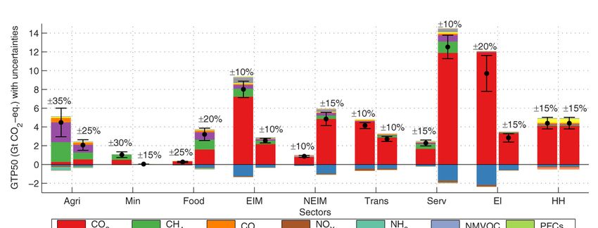
J. Karstensen et al.: Current consumption-based emissions estimates                                                                                                                           289

sumption, which are potentially geographically separated,                                                                                                      Uncertainty relative to initial value
                                                                                                                                                               Trendline relative to initial values
and estimates the consumption that is driving current produc-                        5
                                                                                    10                                                                         Uncertainty relative to final value
                                                                                                                                                               Trendline relative to final values
tion emissions and hence future global temperature response.                                                         R2 of initial values: 0.94549

   All data sets and models introduce uncertainties in the                           4
                                                                                    10
analysis, and thus we estimate uncertainties in the economic

                                                                  Uncertainty (%)
data, the emissions data, and metric parameters in order to es-
timate uncertainties in the final results. We undertake the un-                      3
                                                                                    10

certainty analysis using Monte Carlo (MC) analysis, in which
                                                                                                         R2 of final values: 0.99662
data sets and parameters are randomly perturbed according to                         2
                                                                                    10
predetermined distributions, and then sub-models are run se-
quentially to obtain distributions of the results (Granger Mor-
gan et al., 1990). We isolate the individual contributions to                        1
                                                                                    10

uncertainty in the final results by perturbing individual com-                       10
                                                                                         −3          −2
                                                                                                    10                10
                                                                                                                        −1
                                                                                                                                       10
                                                                                                                                          0                1
                                                                                                                                                          10              10
                                                                                                                                                                             2
                                                                                                                                                                                            10
                                                                                                                                                                                               3

                                                                                                                              Sector size (billion dollars)
ponents independently, before running everything together to
estimate total uncertainty. The analysis considers paramet-       Figure 2. Error distribution of selected GTAP input–output data
ric uncertainties for the components, as opposed to structural    (taken from Table 19.6 in McDougall (2006) and shown as colored
uncertainties, which would include the comparisons of dif-        circles), and trend lines showing the fit of the general functional
ferent models and data sets (Peters et al., 2012). The next       relationship explained by Eq. (1). Red and blue circles differ due to
section lists the background data, and shows how uncertain-       different methods of estimating the difference between unbalanced
ties are estimated, before running the models and discussing      and balanced data. See the discussion in the text.
the results.

                                                                  tries, and thus the global uncertainty is mostly a reflection of
2.1   Data sets and models                                        these countries’ data quality (Andres et al., 2012).
We use multi-regional input–output (MRIO) analysis to link           The estimated global temperature impact of emissions
economic activities from production to consumption, cap-          are calculated using the global temperature change potential
turing global supply chains at the sectoral level (Davis and      (GTP) metric (Aamaas et al., 2013; Shine et al., 2005), which
Caldeira, 2010; Wiedmann, 2009). We source our economic           is essentially a parameterization of more complex climate
input–output data from the Global Trade Analysis Project          models. The metric uses pollutant characteristics (atmo-
(GTAP) database version 8, which comprises domestic and           spheric lifetime, radiative forcing (RF)) as input, and unlike
trade data for the entire world economy in 2007 divided           the more commonly used global warming potential (GWP)
into 129 regions and 58 sectors (Narayanan et al., 2012).         which only relates to RF, the GTP also includes estimates
We use these data to construct an MRIO model with the             of climate temperature response (sensitivity) to changed RF
same regional and sectoral resolution, connecting all regions     in the atmosphere, which adds additional layers of uncertain-
at the sector level (Andrew and Peters, 2013; Peters et al.,      ties (Reisinger et al., 2010). We base our pollutant parameters
2011b). While GTAP does not provide uncertainty estimates         on the ATTICA (European Assessment of Transport Impacts
for the economic data sets, it is possible to generate realis-    on Climate Change and Ozone Depletion) assessment (Fu-
tic uncertainty estimates for the GTAP database from proxy        glestvedt et al., 2010) and IPCC (2007, 212–213), and cli-
data. Since an MRIO database is an aggregation of multiple        mate sensitivity and CO2 uncertainties on the latest CMIP5
data sets, it inherits uncertainties from a number of sources,    data (Olivié and Peters, 2013). The uncertainties of the other
including source data, base year extrapolations, balancing        pollutants are drawn from several sources, but mostly follow-
and harmonization procedures, allocations, and aggregations       ing the IPCC Fifth Assessment Report (Myhre et al., 2013a).
(Wiedmann, 2009; Weber, 2008).
   We use emissions data for the year 2007 from the Emis-         2.2                         General uncertainty relationships
sions Database for Global Atmospheric Research (EDGAR)
for a number of pollutants (see Table 1), mapping these data      It has previously been shown that economic and emissions
to the regions and sectors of the GTAP database. Uncertain-       data show a general pattern where relative uncertainty is in-
ties in emission statistics for each pollutant are derived from   versely related to the magnitude of the data point (Lenzen et
multiple sources, e.g., for CO2 : the amount of fuel that is      al., 2010; Wiedmann, 2009; Wiedmann et al., 2008; Lenzen,
actually consumed, its carbon content, and how much of it         2000). The GTAP data used in our analysis follow a similar
is combusted. Additionally, to be consistent with top-down        relationship, based on differences between the reported input
estimates, statistics are subject to adjustments and harmo-       data and the final data in the database after the harmonization
nization, and aggregated and grouped to economic sectors.         and balancing of selected input–output (IO) data (Table 19.6
Although national uncertainty may in some cases be large,         in McDougall, 2006). Figure 2 illustrates the inverse rela-
global emissions are dominated by a small number of coun-         tionship between unbalanced and balanced data in the GTAP

www.earth-syst-dynam.net/6/287/2015/                                                                                Earth Syst. Dynam., 6, 287–309, 2015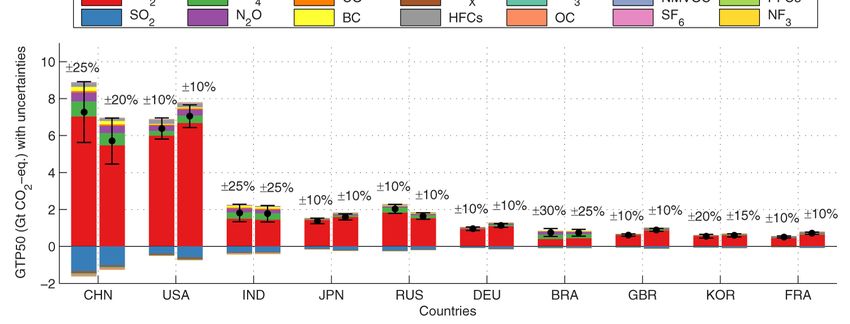
290                                                        J. Karstensen et al.: Current consumption-based emissions estimates

Table 1. Global emissions and uncertainties. The uncertainties indicate the 5–95 % (90 %) percentile range. PFCs include C2F6, C3F8,
C4F10, C5F12, C6F14, C7F16, CF4, and c-C4F8. HFCs include HFC-125, HFC-134a, HFC-143a, HFC-152a, HFC-227ea, HFC-23, HFC-
236fa, HFC-245fa, HFC-32, HFC-365mfc, and HFC-43-10-mee, following UNEP (2012).

               Pollutant   Global emissions (kt)   Uncertainty   Emissions references          Uncertainty references
               PFCs                  1.47 × 101        ±17 %     European Commission (2011)    UNEP (2012)
               CH4                   3.25 × 10⁵        ± 21 %    European Commission (2011)    UNEP (2012)
               CO                    9.47 × 10⁵        ± 25 %    European Commission (2011)    European Commission (2011)
               CO2                   3.14 × 10⁷         ±8%      European Commission (2011)    UNEP (2012)
               HFCs                  2.68 × 10²        ± 17 %    European Commission (2011)    UNEP (2012)
               N2 O                  1.02 × 10⁴        ± 25 %    European Commission (2011)    UNEP (2012)
               NF3                 1.58 × 10⁻¹         ± 26 %    European Commission (2011)    Weiss et al. (2008)
               NH3                   4.92 × 10⁴        ± 25 %    European Commission (2011)    Clarisse et al. (2009)
               NMVOC                 1.60 × 10⁵        ± 50 %    European Commission (2011)    European Commission (2011)
               NOx                   1.27 × 10⁵        ± 25 %    European Commission (2011)    European Commission (2011)
               SF6                   6.17 × 100        ± 10 %    European Commission (2011)    Levin et al. (2010)
               SO2                   1.22 × 10⁵        ± 11 %    European Commission (2011)    Smith et al. (2010)
               BC                    5.22 × 10³        ± 84 %    Shindell et al. (2012)        Bond et al. (2004)
               OC                    1.34 × 10⁴        ± 84 %    Shindell et al. (2012)        Bond et al. (2004)

database together with a first-order regression (R 2 > 0.9).            tainty in the minimum and maximum values)
These differences result from the GTAP harmonization and                     rmin
balancing process and values are only published for a sample            a= b ,                                                      (2)
                                                                             vmax
of “large sectors in large regions with large relative changes”              rmax − rmin
(McDougall, 2006). As a consequence of this data selection              b=               .                                          (3)
                                                                             vmin − vmax
bias, it is not possible to convert these differences directly
to more general sectoral uncertainties. Other uncertainty as-           It is generally argued that developed countries have lower
sessments in MRIO analysis have also taken this inverse rela-           uncertainty than developing countries due to the strength of
tionship as the starting point (Lenzen et al., 2013; Moran and          institutions (Narayanan et al., 2012; Andres et al., 2012). The
Wood, 2014; Lenzen et al., 2012a). Furthermore, a similar re-           terms rmin and rmax define the smallest and largest relative er-
lationship is found with emissions data, based on a previous            rors, respectively, and are functions of developed and devel-
study of the UK Greenhouse Gas Inventory, where uncer-                  oping regions (using the Kyoto Protocol groupings of Annex
tainties were found using an error propagation model (Jack-             B and non-Annex B countries). We assume that developing
son et al., 2009). The underlying mechanisms for this inverse           countries have double the uncertainties of developed coun-
relationship are, however, unclear. The uncertainties may re-           tries, based on estimates for CO2 emissions (Andres et al.,
flect conflicting data sources, unreliable measurements, bias           2012; see further discussion in Sect. 2.4). This range is also
in the source data, allocations and aggregations, base year             sector and region dependent for the economic and emissions
extrapolations, estimates, and assumptions, etc. (Wiedmann,             data, which we define below. The terms vmin and vmax re-
2009; Weber, 2008; Lenzen, 2000), and it is unclear if all              fer to fixed minimum and maximum data values for sectors
these uncertainties will lead to a clear inverse relationship           in a specific region given the uncertainty of rmax and rmin ,
with data values. It may be that the method of generating the           respectively. Figure 3 shows the functional relationship be-
data through some sort of optimization process leads to the             tween sector sizes and uncertainties for economic and emis-
relationship.                                                           sions data.
   The data sets allow for the parameterization of a func-                 The lower threshold vmin is fixed for all regions in the eco-
tion mapping relative uncertainties to the magnitude of the             nomic and emissions data sets, giving sectors of the same
data points. Following previous studies (Lenzen et al., 2010;           size the same uncertainty, as the smallest sectors do not con-
Wiedmann et al., 2008), we assume the data follows a power              tribute much to the national totals. The upper threshold vmax
function                                                                can also be fixed to a certain sector size. However, uncertain-
                                                                        ties are likely to be regionally variable, as while a sector of,
rx = a x b ,                                                     (1)    e.g., USD 1 billion might be very large for some countries, it
                                                                        might not be large in other regions. To account for this, we
where a and b are coefficients. As there is very little data            argue that the sectors’ importance should vary with their con-
available to parameterize Eq. (1), we parameterize the rela-            tribution to the nations’ totals, e.g., gross domestic product
tionship using two extreme data points (generally the uncer-            (GDP) or total emissions. We therefore scale vmax according

Earth Syst. Dynam., 6, 287–309, 2015                                                        www.earth-syst-dynam.net/6/287/2015/
J. Karstensen et al.: Current consumption-based emissions estimates 291
200
Developed regions
300 Developing regions 180
160
250
140
200 120
Uncertainty (%)
Uncertainty (%)
100
150
80
100 60
40
50
20
0 0
0 1 2 3 4 5 6 −6 −4 −2 0 2 4 6
10 10 10 10 10 10 10 10 10 10 10 10 10 10
Sector size (kt emissions) Sector size (M dollar) 0 1 2 3 4 5 6
Figure 3. Functional relationship between sector sizes on the hor- Figure 4. Distributions depending on median values and uncer-
izontal axes (in kt CO2 and million US dollars) and relative uncer- tainty. Both distributions have a median of 1, while the near-normal
tainty on the vertical axes. The red lines outline the range of devel- distribution (green) has a relative uncertainty of 100 %, the skew
oping regions, while the blue lines show the range of developed distribution has a relative uncertainty of 500 %. The green and red
countries. Each region has been estimated using a single unique shaded areas indicate the 5–95 % (90 %) confidence intervals.
curve, and all sectors, depending on their size, will fall on this curve.
The form of this relationship is established independently for each
pollutant. By randomly perturbing each data point, we assume no
correlation in the uncertainties of economic and emissions
data, which might not be accurate for some sector combina-
tions (Peters et al., 2012). Implementing correlations in such
to the regions’ GDP and total emissions, for the respective
an analysis is a major difficulty due to the size of the system
data sets, so that the sectors’ importance in different regions
under investigation and the lack of uncertainty data, but this
is reflected by their uncertainties. Sectoral values larger than
may also have significant effects on the results. We discuss
vmax are given the same uncertainty as values equal to vmax ,
this further in Sect. 4. We do, however, undertake a simple
to ensure that single large sectors do not affect the uncertainty
sensitivity analysis on the parameter choices by comparing
in other large sectors (see details below).
the final results on MRIO uncertainty with uncertainty from
To help illustrate the effects of the methodology, we show
the GTAP table showing extreme observations.
two examples: (1) one of China’s largest economic sectors is
Aggregations of the results (from sectors to regions and
the public administration, defense, education, and health sec-
from regions to the globe) usually decrease the relative un-
tor, worth nearly USD 340 billion in 2007. Large sectors are
certainty, so that the national uncertainty is lower than indi-
given small uncertainties, and this sector is a substantial part
vidual sectors, and global uncertainty is in some cases lower
of China’s GDP (around 10 %). The uncertainty is therefore
than national uncertainty. This is a result of the summation
assumed to be one of the lowest in the country, but scaled
effect, and the relationship between sector sizes and uncer-
up relative to other countries since China is not an Annex-B
tainties. The largest sectors are given the lowest uncertain-
country. (2) One of the USA’s smallest direct CO2 -emitting
ties, so that the national uncertainty is largely a reflection of
sectors is the production of electronic equipment. Emitting
the uncertainty of the largest sectors. As an example of the
roughly 1 Mt CO2 , this is on the lower-end of the scale, con-
summation effect, the relative uncertainty r of adding M ±S,
tributing little to the national total of nearly 5000 Mt CO2 .
n times, is
This sector is therefore given higher relative uncertainty. We
expand on these examples with specific numbers in the next S/M
r= √ , (4)
sections, after we define the uncertainty ranges for the eco- n
nomic and emissions data. assuming no correlations. To illustrate this effect, we show
The estimated uncertainties are used to create distribu- the uncertainty results at multiple levels.
tions of perturbations. We impose lognormal distributions so
that distributions with small relative spreads closely resem-
2.3 Economic data (multi-regional input–output model)
ble normal distributions, while distributions with large rela-
tive spreads are skewed but avoid negative values (Fig. 4). The total sectoral output x of a region’s economy (a vector)
The distributions are characterized using reported data as is the sum of intermediate consumption Ax and final con-
medians, and the spreads are (in order of decreasing pref- sumption, y (Miller and Blair, 1985):
erence) taken directly from the literature, derived from pub-
x = Ax + y, (5)
lished analyses, or estimated. We define uncertainties as the
5–95 % confidence interval (90 % CI; equivalent to 1.64 stan- where A is the inter-industry requirements matrix, which is
dard deviations of a normal distribution). equivalent to the technology used in each sector’s production.
www.earth-syst-dynam.net/6/287/2015/ Earth Syst. Dynam., 6, 287–309, 2015292 J. Karstensen et al.: Current consumption-based emissions estimates
We solve for the total output A value of USD 1 in an input–output table (IOT) is exceed-
−1 ingly small (it represents the economic relationship between
x = (I − A) y, (6)
two sectors over 1 year). Indeed, analysis shows that remov-
where (I − A)−1 is the Leontief inverse L. Emissions are es- ing small values has a negligible effect on the estimates’
timated for a given y by first estimating the output, and then consumption-based emissions (Peters and Andrew, 2012).
linking to sectoral emission intensities, F . This gives the di- Thus, USD 1 is effectively zero in our data set. It could also
rect and indirect emissions (supply chain) emissions be argued that the value of USD 1 is highly uncertain and
should have large uncertainty. Giving values smaller than
f = F Ly. (7)
this higher relative uncertainty causes highly skewed log-
The economic data from GTAP is represented in a multi- normal distributions for the perturbations (see Fig. 4). The
regional input–output (MRIO) model, which is constructed GTAP data set has values as low as 7 × 10⁻³⁵ causing r to be
from a number of smaller data sets. The GTAP data set itself 6 × 10⁶ %. Such highly skewed distributions for data points
is based on a large number of smaller data sets (such as na- with small medians (
USD 1) can lead to large imbalances
tional IO tables and trade data from the UN’s COMTRADE in the table.
database), which are harmonized to remove inconsistencies An IO model is balanced so that gross input equals gross
(Andrew and Peters, 2013; Peters et al., 2011b; Narayanan output, a fundamental characteristic of input–output models
et al., 2012). The construction of an MRIO table from the (Leontief, 1970). The same applies for a multiregional model
GTAP data is explained in detail elsewhere (Peters et al., (MRIO). When perturbing the coefficients in an IO table,
2011b). In the MC analysis, we perturb the components of it ultimately upsets the balance. In principal, the IO table
the GTAP database (e.g., domestic IO data and international can be rebalanced, but given the size of the systems (about
trade data) and not the resulting MRIO. In other words, we 7500 × 7500 matrices), rebalancing is prohibitively compu-
estimate the uncertainty of the MRIO data based on the un- tationally expensive, and may reduce uncertainties as the per-
certainty in the data used to construct it (Peters et al., 2011b), turbed values are changed. We therefore choose not to rebal-
which consists of all data points in the GTAP database used ance, which effectively causes the “unbalanced” component
to construct the MRIO model. This ensures that the uncer- to be shifted to the value added. A concern is that the value
tainties of the final model reflect the underlying uncertainties added may become unrealistic (e.g., negative) as a conse-
of the various input data. We construct the perturbed L and quence. The MC algorithm specifically outputs value added
y, before allocating the direct emissions F (which are also components to allow crosschecking imbalances with the raw
perturbed) to consuming regions and sectors. data, and we find the distributions of the value added at the
We calibrate the uncertainty relationship (Eq. 1) for the sector level to be within expected uncertainty bounds given
GTAP data using several data sets. From the trend lines cre- the size of the value added. This is partially because of the pa-
ated from the GTAP table (Fig. 2), we find the smallest un- rameterization of uncertainty we have used, and partially be-
certainty of the largest sectors to be at approximately 5 %. cause the perturbations tend to cancel out (the sum of random
We therefore let 90 % of perturbed values fall within 5 % of numbers). Thus, we can justify not rebalancing our perturbed
the median, and set rmin = 5 % for the largest sectors (where IOTs and assume the imbalances are allocated to the value
vmax applies). added (without having a large effect on the value added).
The upper threshold vmax is defined by the regions’ GDP Implementing this general methodology has also led to rel-
so that a sector of a specific size will have a larger impor- atively small regional uncertainties in other studies (Lenzen
tance (and hence a lower uncertainty) in a small region than et al., 2010; Wiedmann et al., 2008). Structural uncertain-
in a large region. We use the UK data provided by Lenzen ties have also been found to be relatively small for major
et al. (2010) to explain the range of uncertainties in a single economies (Moran and Wood, 2014). As a simple sensitivity
economy. In this data set the largest sectors have the small- analysis of the input uncertainties, we also run the MC model
est error, and following the trend line we find that the largest with uncertainties according to the fit of the GTAP table un-
value is about 4 % of UK GDP. We use this to define the up- certainties (trend line relative to final values, due to better
per threshold vmax = 4 % × GDPr , which means that sectors fit; Fig. 2). This vastly increases the uncertainties of all sec-
at or above this value will be given the lowest national un- tors, and we do not constrain the upper or lower uncertainties,
certainty (rmin ). Figure 3 shows the result of the implemen- meaning that very small sectors will be given unrealistically
tations, where the lines indicate the range of developing and large uncertainties (USD 1 gives r = 109 %). This exercise
developed regions’ sector sizes and uncertainties. is only valid for the data it represents, large sectors in large
For the smallest sectors we set vmin equal to USD 1 and countries, but is useful for facilitating a discussion about un-
assume rmax = 100 % (following Wiedmann et al., 2008), certainties in economic data. We discuss these results when
due to the lack of more precise regional uncertainty data. exploring MRIO uncertainties, but do not include this when
The USD 1 relates to a small value often used in the GTAP combining uncertainties.
database (Peters, 2006). These parameters may seem some- Expanding on our previous example of the Chinese public
what arbitrary, but these choices are not overly important. administration, defense, education, and health sector, we can
Earth Syst. Dynam., 6, 287–309, 2015 www.earth-syst-dynam.net/6/287/2015/J. Karstensen et al.: Current consumption-based emissions estimates 293
now calculate the uncertainty. Each data point in our MRIO 95 % CI (UNEP, 2012). Global SO2 emissions have an esti-
model consists of inputs from several different GTAP data mated uncertainty of between ±8 and ±14 %, while regional
sets. When these data sets are combined, together with the uncertainties may be as large as ±30 % (Smith et al., 2010).
uncertainties, the MRIO model and its uncertainty are ob- For CH4 , N2 O, and F gases, the uncertainty of global emis-
tained. In the MC analysis, all data sets are given uncertain- sions have been estimated as ±21, ±25, and ±17 %, respec-
ties and perturbations (according to the inverse relationship) tively (UNEP, 2012).
before constructing the MRIO model. The Chinese public ad- Table 1 shows parameters and uncertainties for each pol-
ministration, defense, education, and health sector, which is lutant used as median values in the perturbations. Very little
a single sector in the final GTAP–MRIO model, is built up data exist on the uncertainty of emissions by sector, espe-
from several data sets (bilateral trade, intermediate demand, cially on a pollutant and regional level. Lenzen et al. (2010)
and final demand of households, governments, and capital in- used a table of selected sectors of UK CO2 emissions to find
vestments). In our example, we choose to focus on one of the uncertainties, originating from Jackson et al. (2009). Accord-
most significant contributors to this sector: domestic govern- ing to the regression of the data points, within the limits of
ment consumption expenditure. This sub-data set has a sec- the data points, there is a spread of uncertainties by roughly a
toral range from < 1 to USD 420 billion, which, when cal- factor of 10 (Fig. 2 in Lenzen et al., 2010). We therefore esti-
culating the uncertainty, is constrained in the calculations by mate sectoral uncertainty using the same general relationship
the lower and upper threshold vmin = USD1 and vmax = 4 % as with the economic data (Eq. 1), where the uncertainty of
of national GDP = USD 130 billion. For the uncertainty, the global emissions is used as a proxy for the lowest uncertainty
general sectoral range is rmin = 5 % to rmax = 100 %. GTAP estimate of the largest sectors (rmin ) and the smallest sectors’
estimates the value added in the sector in this sub-data set uncertainty is scaled by 10 times (rmax = 10 rmin ).
to be around USD 340 billion, which is 10 % of national We assign developing countries an rmin and rmax which are
GDP. This is well above vmax , giving this sector a relative double those of developed countries. We define vmin = 1 kt
uncertainty equal to rmin (5 %). Since China is a non-Annex and vmax = 5 % of regional emissions. This dependence on
B country, this is doubled, leading to a final uncertainty of total regional emissions shifts the function so that a sector
10 % for this sector in this sub-data set. The uncertainties for of a specific size will have a larger importance (and hence a
the other data points in the other sub-data sets that make up lower uncertainty) in a smaller region than in a larger region
the Chinese public administration, defense, education, and (Fig. 3). We do not distinguish between different sources of
health sector will be estimated similarly, and together explain the same pollutant, due to a lack of information at the sec-
the overall uncertainty of this sector in the GTAP–MRIO tor level. This is, in some cases, a crude simplification (e.g.,
model. when comparing uncertainties in emissions of certain pol-
lutants from the agricultural sector and power generation).
2.4 Emission statistics
Similarly, for the emissions data, we set vmin equal to 1 kt of
emissions. Values below this (as with economic data) have
The pollutants considered are listed in Table 1, which cover little impact on the footprint of regions and sectors, and are
anthropogenic emissions for the year 2007 which have an ef- therefore given zero uncertainty.
fect on the climate. We do not include emissions from short Expanding on our previous example of emissions from
cycle biomass burning, as this is considered to have a short the USA’s electronic equipment sector, we can now cal-
lifetime in the atmosphere due to regrowth. The data set culate the uncertainty. The USA’s sectors have a range of
originally includes CO2 emissions from forest fires and de- CO2 emissions from 0.3 kt to 2500 Mt, which is then con-
cay, which is a mix of natural and anthropogenic emissions. strained in the calculations by the lower and upper thresh-
Extracting the anthropogenic emissions and mapping them old vmin = 1 kt CO2 and vmax = 5 % of national total CO2 =
to agricultural sectors would require crude assumptions. We 247 Mt CO2 . For CO2 uncertainty, the general sectoral range
therefore do not include emissions related to forest loss, but is from rmin = 16 % (or ±8 %), taken from Table 1, to rmax =
acknowledge that it would increase global CO2 emissions 10×rmin = 160 %. The emissions in the electronic equipment
by roughly 12 % (van der Werf et al., 2009). The EDGAR sector are 1.2 Mt CO2 , which is 0.02 % of total emissions.
data set only provides crude information on uncertainty at the This is in between vmin and vmax , giving the CO2 emissions
global level for some species (European Commission, 2011). from this sector a relative uncertainty of 43 %. Since the USA
Therefore, global and regional uncertainties in emissions are is an Annex B country, this is not doubled.
taken from a variety of sources (Table 1). Global fossil fuel With every sector data point having an uncertainty, we
CO2 emissions statistics are independently produced by sev- create perturbations which we can sum to get a bottom-up
eral organizations, but they generally agree with each other estimate of the national uncertainty. Table 2 shows several
within about 5 % for developed countries and 10 % for de- perturbations of sectors (xin ) for region r. Each perturbation
veloping countries (Andres et al., 2012). The CO2 emission i leads to a new national total (Xi ). However, independent
estimates are all based on energy data, and globally the emis- uncertainty estimates of national totals (e.g., national emis-
sions are thought to have an uncertainty of ±10 % using a sions) that may be available for some regions may conflict
www.earth-syst-dynam.net/6/287/2015/ Earth Syst. Dynam., 6, 287–309, 2015294 J. Karstensen et al.: Current consumption-based emissions estimates
Table 2. Example of perturbations of sectors for a single region r, and the resulting distribution of the national total. This bottom-up
uncertainty estimate may not be consistent with top-down uncertainty estimates.
National total Distribution of
Region r Sector 1 Sector 2 Sector 3 Sector n (sum of sectors) national totals
Perturbation 1 x11 x12 x13 x1n X1
Perturbation 2 x21 x22 x23 x2n X2 → XN
Perturbation 3 x31 x32 x33 x3n X3
Perturbation i xi1 xi2 xi3 xin Xi
with our bottom-up distributions of the national totals (XN ). ing potential (GWP) (Aamaas et al., 2013; Reisinger et al.,
When summing the perturbed sectors xin for a region, it is 2010) and it has been criticized for some of its characteris-
unlikely that the distribution of XN will be the same as the tics (Pierrehumbert, 2014), the GTP directly links to global
known uncertainty in X. temperature change and is thus arguably more policy relevant
Additionally, the uncertainty in X N will depend on the (Shine et al., 2005). In addition, the physical interpretation of
number of elements contributing to the sum, according to the GWP is less clear and the metric has been criticized by
standard propagation of uncertainty rules (RSS, root sum many authors (Peters et al., 2011a; Shine, 2009; Pierrehum-
square; see earlier discussion on the summation effect). In bert, 2014). The GTP metric is calculated using impulse re-
practice, the uncertainty of X may be based on several lines sponse functions, which explain the interaction of pollutant i
of evidence, which may even exclude sector-based data. in the atmosphere (impulse response function; IRFi ) and the
To ensure that we can reproduce the top-down uncertainty climate system (temperature) response to a pulse emission
estimates of X, we use constrained optimization (using a (IRFT ) with specific RF and atmospheric lifetime.
quadratic programming (QP) methodology) to minimally ad- We briefly describe the metric equations here, and refer
just the perturbations of xin to a given distribution of the XN to existing literature for more details (Aamaas et al., 2013;
(Table 2). Fuglestvedt et al., 2010; Olivié and Peters, 2013; Myhre et
Given that we can adjust one iteration so that it sums to a al., 2013b). The absolute GTP (AGTP) for each pollutant i is
fixed X, we then give X a distribution based on known na- defined as
tional uncertainties, and thus, each iteration of X is used to
balance the same iteration of the disaggregated sector data ZH
(xin ). This ensures that the sum of sectors (Xi ) always gives AGTPi (H ) = RFi (t) IRFT (H − t) dt, (8)
a XN with a known uncertainty. The cost of this adjustment is 0
that the spread of the large values in each region (e.g., a large
sector) are adjusted to fit the constraints. To meet the criteria where the RF for a pulse emission is
of, e.g., a narrower distribution of the aggregated values, the
t
large values have to be given a narrower distribution as well. RFi (t) = RE × IRFi = Ai exp − , (9)
This methodology allows us to give realistic uncertainties for τi
each xin leading to an XN with a known uncertainty. We do
where t is time (years), H is the time horizon (years), Ai is
not perform such balancing on the MRIO input data (previ-
the radiative efficiency for pollutant i (W (m−2 kg)), and τi is
ous section) as it is too computationally expensive, and there
the decay time for pollutant i (years). The AGTP metric is
is little top-down data on uncertainties in economic data.
dependent on the IRF of temperature, which incorporates the
climate system response in global-mean surface temperature
2.5 Emission metrics to a given RF. The climate response is modeled using two
To link emissions to temperature change, we use the global decaying exponential functions representing (1) the relative
temperature change potential (GTP) as a metric to compare fast response of the atmosphere, the land surface, and the
and aggregate pollutants (Shine et al., 2007). This gives an ocean mixed layer, and (2) the relative slow response of the
estimate of the global-mean surface temperature change due deep ocean (Peters et al., 2011a),
to a pulse of emissions from a specific pollutant, and is a J
simple way of modeling the much more complex climate
X cj t
IRFT = exp − , (10)
system and its response. Uncertainties in metric values can d
j =1 j
dj
arise from a number of factors, including pollutant parame-
ters (RF and lifetime) and the response of the climate system. where J is the number of decay terms (usually two), cj is
Although it has been shown that the GTP may have larger rel- a component of the climate sensitivity
P (K (Wm−2 )), where
ative uncertainties than the alternative metric global warm- the total climate sensitivity λ = cj , and dj is the decay
Earth Syst. Dynam., 6, 287–309, 2015 www.earth-syst-dynam.net/6/287/2015/J. Karstensen et al.: Current consumption-based emissions estimates 295
Table 3. Metric parameters with uncertainties. Note that the uncertainties are derived from CMIP5 data and Joos et al. (2013), but we use
the corresponding distributions listed in Table 5 and 6 in the study by Olivié and Peters (2013) to account for correlations.
Parameters Values Unit Uncertainties
Climate sensitivity f1 0.43 K Wm−2 ±29 %
Climate sensitivity f2 0.32 ±59 %
Climate sensitivity decay τ1 2.57 year ±46 %
Climate sensitivity decay τ2 82.24 ±192 %
CO2 weight a0 0.23 ±20 %
CO2 weight a1 0.28 ±33 %
CO2 weight a2 0.35 ±28 %
CO2 weight a3 0.14 ±30 %
CO2 decay τ0 Infinite year –
CO2 decay τ1 239.6 ±58 %
CO2 decay τ2 18.42 ±68 %
CO2 decay τ3 1.64 ±63 %
time (years) of component cj . These two functions are ex- temperature results was found to be small (less than 1 % of
plained by lifetime and climate sensitivity for the individual AGTP50 value for CO2 ).
components (Table 3). The λ explains the change in equi- Estimates from the literature are used as the median (Fu-
librium global-mean temperature due to forcing by a pollu- glestvedt et al., 2010) and estimates of uncertainty as spread
tant in the atmosphere. We parameterize the IRF according to of the distributions (Tables 4 and 5). For the non-reactive
the results from CMIP5 covering 15 different climate models pollutants, we randomized the single RF and lifetime val-
(Olivié and Peters, 2013). This data set is parameterized by ues, as these are represented by only a single decay func-
relatively short climate runs (140–150 years), and thus it is tion. The RF used in the calculations includes the indirect
more representative of the short-term climate response (less effects of chemical reactions from the ozone precursors (CO,
than 100 years) compared to the equilibrium response (see NOx , and NMVOC), which were perturbed similarly as the
Olivié and Peters, 2013 for details). Nevertheless, the data other pollutants. This accounts for three indirect forcing ef-
set leads to a median λ = 0.75 K Wm−2 (equivalent to 2.8 ◦ C fects: formation of O3 (causing positive RF by CO, NOx , and
global-mean temperature increase), which is consistent with NMVOC), changing CH4 levels (causing positive RF by CO
the climate response (sensitivity) of a doubling of CO2 con- and NMVOC, and negative RF by NOx ), and CH4 -induced
centration in the atmosphere within the range of 1.5 to 4.5 ◦ C O3 effects (causing positive RF from CO and NMVOC, and
(IPCC, 2013). negative RF from NOx ) (Aamaas et al., 2013). The indirect
As CO2 has a more complex interaction in the atmosphere effect of SO2 is included by scaling the metric value, where
and can not be sufficiently modeled with a single exponential the indirect effect of SO2 is estimated to be about 175 % of
decay, we define the RF for CO2 as a sum of exponentials the direct effect (Aamaas et al., 2013). This is a crude es-
(Aamaas et al., 2013): timate, and while the indirect effect may be more uncertain
than the direct effect, we use the same uncertainty for the di-
rect and indirect effects due to lack of pollutant specific data
( )
I
X t
RFCO2 (t) = ACO2 a0 + ai 1 − exp − , (11) (Boucher et al., 2013).
τi
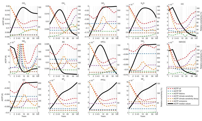
i=1 Our analysis of uncertainty contributions from emissions
and metric parameters uses absolute GTP (AGTP) values
where ai is the weight ofP each exponential, which by defi- with units of temperature change (in Kelvin or ◦ C). When
nition has to sum to one ( ai = 1), and I is the number of later allocating temperature data in the economic model, we
exponentials. We follow Joos et al. (2013) and use four ex- also use GTP values in units of CO2 -equivalent (eq.) emis-
ponentials and weights, and randomize the multiple lifetimes sions for comparison. The GTP values are calculated by nor-
and coefficients so that the coefficients always sum to 1, fol- malizing the AGTP values with reference to the AGTP val-
lowing Olivié and Peters (2013). The use of four different ues for CO2 . When we connect the components for a full MC
timescales was found to be sufficient to model CO2 behav- analysis, we choose a single time horizon for computational
ior in the atmosphere compared to advanced climate models reasons. As discussed elsewhere (Fuglestvedt et al., 2010),
(Olivié and Peters, 2013). Correlations between the param- choosing a time horizon includes value judgment, and is not
eters were implemented for CO2 and IRFT , also based on based solely on a scientific judgment. We choose to focus on
Olivié and Peters (2013), but the effect of the correlations on
www.earth-syst-dynam.net/6/287/2015/ Earth Syst. Dynam., 6, 287–309, 2015296 J. Karstensen et al.: Current consumption-based emissions estimates
Table 4. RF values and uncertainties. Note that CO, non-methane volatile organic compound (NMVOC) and NOx are precursors, which
have an effect on O3 and CH4 concentrations. Because of this, no single RF value can be given. The uncertainties indicate the 5–95 % (90 %)
percentile range. Parameters from IPCC (2007, Table 2.14, p. 212–213).
Pollutant RF (Wm−2 kg−1 ) Uncertainty RF references Uncertainty references
PFCs 6.40 × 10⁻¹² –1.06 × 10⁻¹¹ ±10 % IPCC (2007) Myhre et al. (2013a)
CH4 1.82 × 10⁻¹³ ±17 % Fuglestvedt et al. (2010) Myhre et al. (2013a)
CO – ±24 % Derwent et al. (2001) Myhre et al. (2013a)
CO2 1.81 × 10⁻¹⁵ ±10 % Fuglestvedt et al. (2010) Myhre et al. (2013a)
HFCs 6.74 × 10⁻¹² –1.53 × 10⁻¹¹ ±10 % Fuglestvedt et al. (2010), IPCC (2007) Myhre et al. (2013a)
N2 O 3.88 × 10⁻¹³ ±17 % Fuglestvedt et al. (2010) Myhre et al. (2013a)
NF3 1.66 × 10⁻¹¹ ±10 % IPCC (2007) Assumed
NH3 −1.03 × 10⁻¹⁰ ±123 % Shindell et al. (2009) Myhre et al. (2013a)
NMVOC – ±41 % Collins et al. (2002) Myhre et al. (2013a)
NOx – ±120 % Wild et al. (2001) Myhre et al. (2013a)
SF6 2.00 × 10⁻¹¹ ±10 % Fuglestvedt et al. (2010) Myhre et al. (2013a)
Sulphate −3.20 × 10⁻¹⁰ ±50 % Fuglestvedt et al. (2010) Myhre et al. (2013a)
BC 1.96 × 10⁻⁹ ±66 % Fuglestvedt et al. (2010) Myhre et al. (2013a)
OC −2.90 × 10⁻¹⁰ ±68 % Fuglestvedt et al. (2010) Myhre et al. (2013a)
Table 5. Lifetimes and uncertainties. Uncertainties for several gases’ lifetimes are assumed, but a sensitivity analysis revealed that a change
of this uncertainty will not have a large impact on the results (see metric results section below). Note that CO, NMVOC, and NOx are
precursors, which have an effect on O3 and CH4 concentrations. Because of this, no single lifetime can be given. Values and uncertainties
for CO2 are given in Table 3. The uncertainties indicate the 5–95 % (90 %) percentile range. Parameters from IPCC (2007, Table 2.14,
p. 212–213).
Pollutant Lifetime (years) Uncertainty Lifetime references Uncertainty references
PFCs 2600–50 000 ±20 % Fuglestvedt et al. (2010) Assumed
CH4 12 ±19 % Fuglestvedt et al. (2010) Myhre et al. (2013a)
CO – ±20 % Fuglestvedt et al. (2010) Assumed
CO2 – – Fuglestvedt et al. (2010) –
HFCs 1.4–270 ±12–±29 % Fuglestvedt et al. (2010), Myhre et al. (2013a),
IPCC (2007) Ko et al. (2013)
N2 O 114 ±13 % Fuglestvedt et al. (2010) Myhre et al. (2013a)
NF3 740 ±13 % Fuglestvedt et al. (2010) Ko et al. (2013)
NH3 0.02 ±20 % Fuglestvedt et al. (2010) Assumed
NMVOC – ±20 % Fuglestvedt et al. (2010) Assumed
NOx – ±20 % Fuglestvedt et al. (2010) Assumed
SF6 3200 ±20 % Fuglestvedt et al. (2010) Assumed
Sulphate 0.01 ±20 % Fuglestvedt et al. (2010) Assumed
BC 0.02 ±20 % Fuglestvedt et al. (2010) Assumed
OC 0.02 ±20 % Fuglestvedt et al. (2010) Assumed
the impact at 50 years (AGTP50 and GTP50), as this is both bining them all together (Fig. 1). We first show uncertainties
consistent with current literature (Myhre et al., 2013b), and resulting from (1) the economic data only, (2) the emissions
within reasonable time for when to expect global warming to data only, and (3) the metric calculations only. The final sec-
exceed 2 ◦ C (Joshi et al., 2011; Peters et al., 2013). tion, (4), connects these three parts together to follow uncer-
tainty through the entire cause–effect chain. The results show
uncertainty propagation from consumption to global temper-
3 Results
ature change. The analysis is based on 10 000 MC runs.
Estimated uncertainties are used to create distributions of all
data points. To analyze how various stages of the cause–
effect chain contribute to overall uncertainty, we introduce
uncertainty separately in each part of the chain before com-
Earth Syst. Dynam., 6, 287–309, 2015 www.earth-syst-dynam.net/6/287/2015/J. Karstensen et al.: Current consumption-based emissions estimates 297
3.1 MRIO uncertainty Since we start from the raw GTAP data to construct the
MRIO table, and normalize and invert the MRIO table, a vast
number of summations and multiplications are done with the
In this section, we assume there are no uncertainties in the initial perturbed data (an inversion in a single MC ensem-
territorial emissions data or emission metrics, and thus the ble requires more than 1012 operations, which was estimated
MRIO model uses unperturbed median estimates of GTP50 using the Lightspeed Matlab toolbox; Minka, 2014). Follow-
values for all pollutants when allocating emissions to con- ing RSS uncertainty propagation, the relative uncertainty will
sumers, and uncertainties are purely dependent on parametric decrease when adding equally sized numbers with equally
uncertainty in the input data into the MRIO. In our analysis, sized uncertainty (not an unrealistic assumption for input–
each of the 129 countries has 57 producing sectors (not in- output analysis). Thus, the relative uncertainty of the sum of
cluding households as they are considered final demand in a row in the MRIO (the output) will depend on the number,
the model, and therefore not included in the processing), and n, of large data points (Eq. 4). This problem can be avoided
thus the MRIO table has 7353 rows and columns. We em- by using a quadratic programming approach to rebalance the
phasize here, but discuss later, that we consider parametric sum to a given uncertainty (as we do for the emissions data),
uncertainties and not structural uncertainties. but we do not do this as (a) it is too computationally expen-
Table 6 shows uncertainties in emissions embodied in im- sive, and (b) it would require balancing the entire MRIO table
ports and exports, as well as consumption, due to pertur- to get consistent sums. This problem is difficult to negotiate
bations only on the economic data set. The exports indi- given the size of the database we are using, and consequently
cate goods that are produced domestically but consumed this exerts a downward pressure on MRIO uncertainties. Be-
abroad, while the imports indicate goods produced abroad cause of this, and because uncertainty ranges of input values
but consumed domestically. The uncertainties in exported are small for the largest and most important sectors, the final
emissions are solely due to uncertainties in domestic eco- results have small uncertainties. A valid question is then how
nomic data, thus reflecting the pattern of developed countries reliable the uncertainties are.
having higher uncertainties. Uncertainties in imported emis- The “unfitted” and “fitted” data from Table 19.6 in the
sion are generally higher than exported emissions, as the im- GTAP documentation (Fig. 2) act as a simple sensitivity anal-
ports come from a number of different regions of which many ysis to our applied uncertainties; however, since this table
may have high uncertainties (e.g., emerging and developing only samples the very largest deviations, it is not represen-
economies). tative of the uncertainties in the entire database. When we
For the largest consumption paths, the consumption per- use these, we find that the uncertainties are much larger
spective is not substantially more uncertain than the cor- for the largest emitters (between 160 and 400 % uncer-
responding territorial view due to economic uncertainties. tainty for consumption-based emissions), and for small- and
Following the largest international fluxes embodied in trade medium-sized countries the uncertainties becomes unrealisti-
from Davis and Caldeira (2010) aggregated over all sectors, cally large. Thus, the results are clearly sensitive to the input
we find 2 % uncertainty in emissions embodied in products uncertainties. This is expected as the input uncertainties are
exported from China to the USA, 2 % uncertainty from China outliers in the GTAP database, and thus the uncertainties are
to western Europe, 3 % from China to Japan, and 1 % from known to be large. As a consequence, the vastly perturbed
the USA to western Europe from economic uncertainties values lead to ill-defined MRIO tables (outside of machine
only. These fluxes are mainly dominated by the largest sec- precision), which will compromise the accuracy of the final
tors, to which our method has assigned the smallest uncer- results (see discussion on skew distributions and small data
tainties. The export from China to the USA mainly originates points in the Methods section). However, as discussed ear-
in the manufacturing sectors, which combined is one of the lier, using the difference between input and output values as
largest Chinese sectors, therefore with relatively low uncer- a proxy of uncertainty is not straightforward. For example,
tainties. Annex B countries are assigned lower uncertainties the first data point in Table 19.6 indicates an input values of
than non-Annex B countries, which explains the relatively USD 2 billion and an output value of USD 132 billion, where
low uncertainty from the USA to western Europe. the difference (relative to the initial value) can be interpreted
For smaller paths, there are much higher economic uncer- as a change of 6500 %. This uncertainty is vast, and many
tainties. More than 20 % of the international trade routes have data points have much larger differences. Because of these
a higher uncertainty than 10 % (total number of trade routes difficulties, and since the results are only valid for specific
is 128 regions × 128 regions), while the median of all is 6 % sectors, we do not show regional results from this analysis,
uncertainty. The uncertainties in consumption emissions for but only use it for illustrative purposes.
the top emitters are very low for two reasons: (1) the effect of Overall, we find small uncertainties in the MRIO results;
summations and aggregations reduce the uncertainties on the however, the uncertainties in the end results are a function
national level (Eq. 4; much higher values are seen on a sec- of the uncertainties in the input values, as shown by the sen-
toral level), and (2) the distributions we give the perturbed sitivity analysis. Furthermore, the input uncertainties are es-
data in the larger sectors are relatively small. timated from small amounts of data and many assumptions,
www.earth-syst-dynam.net/6/287/2015/ Earth Syst. Dynam., 6, 287–309, 2015You can also read