Modeling Player and Team Performance in Basketball
←
→
Page content transcription
If your browser does not render page correctly, please read the page content below
Modeling Player and Team Performance in Basketball
                                                                          Zachary Terner1 and Alexander Franks2
                                           1
                                             Department of Statistics and Applied Probability, University of California Santa Barbara,
                                                                  Santa Barbara, CA, 93106; zterner@ucsb.edu
                                           2
                                             Department of Statistics and Applied Probability, University of California Santa Barbara,
                                                              Santa Barbara, CA, 93106; afranks@pstat.ucsb.edu
arXiv:2007.10550v1 [stat.AP] 21 Jul 2020

                                                                                           July 22, 2020

                                                                                              Abstract
                                                   In recent years, analytics has started to revolutionize the game of basketball: quantitative analyses
                                               of the game inform team strategy, management of player health and fitness, and how teams draft, sign,
                                               and trade players. In this review, we focus on methods for quantifying and characterizing basketball
                                               gameplay. At the team level, we discuss methods for characterizing team strategy and performance,
                                               while at the player level, we take a deep look into a myriad of tools for player evaluation. This includes
                                               metrics for overall player value, defensive ability, and shot modeling, and methods for understanding
                                               performance over multiple seasons via player production curves. We conclude with a discussion on the
                                               future of basketball analytics, and in particular highlight the need for causal inference in sports.

                                                                                                   1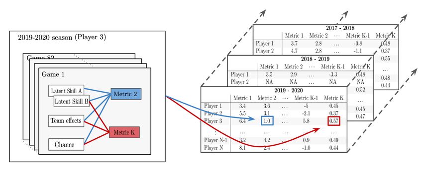
1     Introduction
Basketball is a global and growing sport with interest from fans of all ages. This growth has coincided with
a rise in data availability and innovative methodology that has inspired fans to study basketball through a
statistical lens. Many of the approaches in basketball analytics can be traced to pioneering work in base-
ball (Schwartz, 2013), beginning with Bill James’ publications of The Bill James Baseball Abstract and the
development of the field of “sabermetrics” (James, 1984, 1987, 2010). James’ sabermetric approach capti-
vated the larger sports community when the 2002 Oakland Athletics used analytics to win a league-leading
102 regular season games despite a prohibitively small budget. Chronicled in Michael Lewis’ Moneyball, this
story demonstrated the transformative value of analytics in sports (Lewis, 2004).
    In basketball, Dean Oliver and John Hollinger were early innovators who argued for evaluating players on a
per-minute basis rather than a per-game basis and developed measures of overall player value, like Hollinger’s
Player Efficiency Rating (PER) (Oliver, 2004, Hollinger, 2005a,b). The field of basketball analytics has
expanded tremendously in recent years, even extending into popular culture through books and articles by
data-journalists like Nate Silver and Kirk Goldsberry, to name a few (Silver, 2012, Goldsberry, 2019). In
academia, interest in basketball analytics transcends the game itself, due to its relevance in fields such as
psychology (Gilovich et al., 1985, Vaci et al., 2019, Price & Wolfers, 2010), finance and gambling (Brown &
Sauer, 1993, Gandar et al., 1998), economics (see, for example, the Journal of Sports Economics), and sports
medicine and health (Drakos et al., 2010, DiFiori et al., 2018).
    Sports analytics also has immense value for statistical and mathematical pedagogy. For example, Drazan
et al. (2017) discuss how basketball can broaden the appeal of math and statistics across youth. At more
advanced levels, there is also a long history of motivating statistical methods using examples from sports,
dating back to techniques like shrinkage estimation (e.g. Efron & Morris, 1975) up to the emergence of
modern sub-fields like deep imitation learning for multivariate spatio-temporal trajectories (Le et al., 2017).
Adjusted plus-minus techniques (Section 3.1.1) can be used to motivate important ideas like regression
adjustment, multicollinearity, and regularization (Sill, 2010).

1.1    This review
Our review builds on the early work of Kubatko et al. (2007) in “A Starting Point for Basketball Analyt-
ics,” which aptly establishes the foundation for basketball analytics. In this review, we focus on modern
statistical and machine learning methods for basketball analytics and highlight the many developments in
the field since their publication nearly 15 years ago. Although we reference a broad array of techniques,
methods, and advancements in basketball analytics, we focus primarily on understanding team and player
performance in gameplay situations. We exclude important topics related to drafting players (e.g. McCann,
2003, Groothuis et al., 2007, Berri et al., 2011, Arel & Tomas III, 2012), roster construction, win probability
models, tournament prediction (e.g. Brown et al., 2012, Gray & Schwertman, 2012, Lopez & Matthews,
2015, Yuan et al., 2015, Ruiz & Perez-Cruz, 2015, Dutta et al., 2017, Neudorfer & Rosset, 2018), and issues
involving player health and fitness (e.g. Drakos et al., 2010, McCarthy et al., 2013). We also note that much
of the literature pertains to data from the National Basketball Association (NBA). Nevertheless, most of
the methods that we discuss are relevant across all basketball leagues; where appropriate, we make note of
analyses using non-NBA data.
    We assume some basic knowledge of the game of basketball, but for newcomers, NBA.com provides a
useful glossary of common NBA terms (National Basketball Association, 2014). We begin in Section 1.2 by
summarizing the most prevalent types of data available in basketball analytics. The online supplementary
material highlights various data sources and software packages. In Section 2 we discuss methods for modeling
team performance and strategy. Section 3 follows with a description of models and methods for understanding
player ability. We conclude the paper with a brief discussion on our view on the future of basketball analytics.

1.2    Data and tools
Box score data: The most available datatype is box score data. Box scores, which were introduced by
Henry Chadwick in the 1900s (Pesca, 2009), summarize games across many sports. In basketball, the box
score includes summaries of discrete in-game events that are largely discernible by eye: shots attempted and

                                                       2
made, points, turnovers, personal fouls, assists, rebounds, blocked shots, steals, and time spent on the court.
Box scores are referenced often in post-game recaps.
Basketball-reference.com, the professional basketball subsidiary of sports-reference.com, contains
preliminary box score information on the NBA and its precursors, the ABA, BAA, and NBL, dating back to
the 1946-1947 season; rebounds first appear for every player in the 1959-60 NBA season (Sports Reference
LLC, 2016). There are also options for variants on traditional box score data, including statistics on a per
100-possession, per game, or per 36-minute basis, as well as an option for advanced box score statistics.
Basketball-reference additionally provides data on the WNBA and numerous international leagues. Data on
further aspects of the NBA are also available, including information on the NBA G League, NBA executives,
referees, salaries, contracts, and payrolls as well as numerous international leagues. One can find similar
college basketball information on the sports-reference.com/cbb/ site, the college basketball subsidiary of
sports-reference.com.
For NBA data in particular, NBA.com contains a breadth of data beginning with the 1996-97 season (NBA,
2020). This includes a wide range of summary statistics, including those based on tracking information, a
defensive dashboard, ”hustle”-based statistics, and other options. NBA.com also provides a variety of tools
for comparing various lineups, examining on-off court statistics, and measuring individual and team defense
segmented by shot type, location, etc. The tools provided include the ability to plot shot charts for any
player on demand.
Tracking data: Around 2010, the emergence of “tracking data,” which consists of spatial and temporally
referenced player and game data, began to transform basketball analytics. Tracking data in basketball fall
into three categories: player tracking, ball tracking, and data from wearable devices. Most of the basketball
literature that pertains to tracking data has made use of optical tracking data from SportVU through Stats,
LLC and Second Spectrum, the current data provider for the NBA. Optical data are derived from raw video
footage from multiple cameras in basketball arenas, and typically include timestamped (x, y) locations for
all 10 players on the court as well as (x, y, z) locations for the basketball at over 20 frames per second.1
Many notable papers from the last decade use tracking data to solve a range of problems: evaluating defense
(Franks et al., 2015b), constructing a “dictionary” of play types (Miller & Bornn, 2017), evaluating expected
value of a possession (Cervone et al., 2014), and constructing deep generative models of spatio-temporal
trajectory data (Yu, 2010, Yue et al., 2014, Le et al., 2017). See Bornn et al. (2017) for a more in-depth
introduction to methods for player tracking data.
Recently, high resolution technology has enabled (x, y, z) tracking of the basketball to within one centime-
ter of accuracy. Researchers have used data from NOAH (Marty, 2020) and RSPCT (Moravchik, 2020), the
two largest providers of basketball tracking data, to study several aspects of shooting performance (Marty,
2018, Marty & Lucey, 2017, Bornn & Daly-Grafstein, 2019, Shah & Romijnders, 2016, Harmon et al., 2016),
see Section 3.3.1. Finally, we also note that many basketball teams and organizations are beginning to
collect biometric data on their players via wearable technology. These data are generally unavailable to the
public, but can help improve understanding of player fitness and motion (Smith, 2018). Because there are
few publications on wearable data in basketball to date, we do not discuss them further.
Data sources and tools: For researchers interested in basketball, we have included two tables in the
supplementary material. Table 1 contains a list of R and Python packages developed for scraping basketball
data, and Table 2 enumerates a list of relevant basketball data repositories.
2 Team performance and strategy
Sportswriters often discuss changes in team rebounding rate or assist rate after personnel or strategy changes,
but these discussions are rarely accompanied by quantitative analyses of how these changes actually affect
the team’s likelihood of winning. Several researchers have attempted to address these questions by inves-
tigating which box score statistics are most predictive of team success, typically with regression models
(Hofler & Payne, 2006, Melnick, 2001, Malarranha et al., 2013, Sampaio et al., 2010). Unfortunately, the
practical implications of such regression-based analyses remains unclear, due to two related difficulties in
1A sample of SportVU tracking data can currently be found on Github (Linou, 2016b).
3interpreting predictors for team success: 1) multicollinearity leads to high variance estimators of regression
coefficients (Ziv et al., 2010) and 2) confounding and selection bias make it difficult to draw any causal
conclusions. In particular, predictors that are correlated with success may not be causal when there are
unobserved contextual factors or strategic effects that explain the association (see Figure 3 for an interest-
ing example). More recent approaches leverage spatio-temporal data to model team play within individual
possessions. These approaches, which we summarize below, can lead to a better understanding of how teams
achieve success.
2.1 Network models
One common approach to characterizing team play involves modeling the game as a network and/or modeling
transition probabilities between discrete game states. For example, Fewell et al. (2012) define players as nodes
and ball movement as edges and compute network statistics like degree and flow centrality across positions
and teams. They differentiate teams based on the propensity of the offense to either move the ball to their
primary shooters or distribute the ball unpredictably. Fewell et al. (2012) suggest conducting these analyses
over multiple seasons to determine if a team’s ball distribution changes when faced with new defenses. Xin
et al. (2017) use a similar framework in which players are nodes and passes are transactions that occur on
edges. They use more granular data than Fewell et al. (2012) and develop an inhomogeneous continuous-time
Markov chain to accurately characterize players’ contributions to team play.
Skinner & Guy (2015) motivate their model of basketball gameplay with a traffic network analogy, where
possessions start at Point A, the in-bounds, and work their way to Point B, the basket. With a focus
on understanding the efficiency of each pathway, Skinner proposes that taking the highest percentage shot
in each possession may not lead to the most efficient possible game. He also proposes a mathematical
justification of the “Ewing Theory” that states a team inexplicably plays better when their star player is
injured or leaves the team (Simmons, 2001), by comparing it to a famous traffic congestion paradox (Skinner,
2010). See Skinner & Goldman (2015) for a more thorough discussion of optimal strategy in basketball.
2.2 Spatial perspectives
Many studies of team play also focus on the importance of spacing and spatial context. Metulini et al. (2018)
try to identify spatial patterns that improve team performance on both the offensive and defensive ends of
the court. The authors use a two-state Hidden Markov Model to model changes in the surface area of the
convex hull formed by the five players on the court. The model describes how changes in the surface area are
tied to team performance, on-court lineups, and strategy. Cervone et al. (2016a) explore a related problem
of assessing the value of different court-regions by modeling ball movement over the course of possessions.
Their court-valuation framework can be used to identify teams that effectively suppress their opponents’
ability to control high value regions.
Spacing also plays a crucial role in generating high-value shots. Lucey et al. (2014) examined almost
20,000 3-point shot attempts from the 2012-2013 NBA season and found that defensive factors, including
a “role swap” where players change roles, helped generate open 3-point looks. In related work, D’Amour
et al. (2015) stress the importance of ball movement in creating open shots in the NBA. They show that
ball movement adds unpredictability into offenses, which can create better offensive outcomes. The work of
D’Amour and Lucey could be reconciled by recognizing that unpredictable offenses are likely to lead to “role
swaps”, but this would require further research. Sandholtz et al. (2019) also consider the spatial aspect of
shot selection by quantifying a team’s “spatial allocative efficiency,” a measure of how well teams determine
shot selection. They use a Bayesian hierarchical model to estimate player FG% at every location in the half
court and compare the estimated FG% with empirical field goal attempt rates. In particular, the authors
identify a proposed optimum shot distribution for a given lineup and compare the true point total with the
proposed optimum point total. Their metric, termed Lineup Points Lost (LPL), identifies which lineups and
players have the most efficient shot allocation.
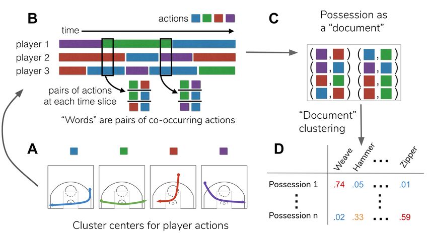
4Figure 1: Unsupervised learning for play discovery (Miller & Bornn, 2017). A) Individual player actions are
clustered into a set of discrete actions. Cluster centers are modeled using Bezier curves. B) Each possession
is reduced to a set of co-occurring actions. C) By analogy, a possession can be thought of as a “document”
consisting of “words.” “Words” correspond to all pairs of co-occurring actions. A “document” is the possession,
modeled using a bag-of-words model. D) Possessions are clustered using Latent Dirichlet Allocation (LDA).
After clustering, each possession can be represented as a mixture of strategies or play types (e.g. a “weave”
or “hammer” play).
2.3 Play evaluation and detection
Finally, Lamas et al. (2015) examine the interplay between offensive actions, or space creation dynamics
(SCDs), and defensive actions, or space protection dynamics (SPDs). In their video analysis of six Barcelona
F.C. matches from Liga ACB, they find that setting a pick was the most frequent SCD used but it did
not result in the highest probability of an open shot, since picks are most often used to initiate an offense,
resulting in a new SCD. Instead, the SCD that led to the highest proportion of shots was off-ball player
movement. They also found that the employed SPDs affected the success rate of the SCD, demonstrating
that offense-defense interactions need to be considered when evaluating outcomes.
Lamas’ analysis is limited by the need to watch games and manually label plays. Miller and Bornn
address this common limitation by proposing a method for automatically clustering possessions using player
trajectories computed from optical tracking data (Miller & Bornn, 2017). First, they segment individual
player trajectories around periods of little movement and use a functional clustering algorithm to cluster
individual segments into one of over 200 discrete actions. They use a probabilistic method for clustering
player trajectories into actions, where cluster centers are modeled using Bezier curves. These actions serve
as inputs to a probabilistic clustering model at the possession level. For the possession-level clustering, they
propose Latent Dirichlet Allocation (LDA), a common method in the topic modeling literature (Blei et al.,
2003). LDA is traditionally used to represent a document as a mixture of topics, but in this application, each
possession (“document”) can be represented as a mixture of strategies/plays (“topics”). Individual strategies
consist of a set of co-occurring individual actions (“words”). The approach is summarized in Figure 1. This
approach for unsupervised learning from possession-level tracking data can be used to characterize plays or
motifs which are commonly used by teams. As they note, this approach could be used to “steal the opponent’s
playbook” or automatically annotate and evaluate the efficiency of different team strategies. Deep learning
models (e.g. Le et al., 2017, Shah & Romijnders, 2016) and variational autoencoders could also be effective
for clustering plays using spatio-temporal tracking data.
It may also be informative to apply some of these techniques to quantify differences in strategies and
styles around the world. For example, although the US and Europe are often described as exhibiting different
5Figure 2: Diagram of the sources of variance in basketball season metrics. Metrics reflect multiple latent
player attributes but are also influenced by team ability, strategy, and chance variation. Depending on the
question, we may be interested primarily in differences between players, differences within a player across
seasons, and/or the dependence between metrics within a player/season. Player 2 in 2018-2019 has missing
values (e.g. due to injury) which emphasizes the technical challenge associated with irregular observations
and/or varying sample sizes.
styles (Hughes, 2017), this has not yet been studied statistically. Similarly, though some lessons learned from
NBA studies may apply to The EuroLeague, the aforementioned conclusions about team strategy and the
importance of spacing may vary across leagues.
3 Player performance
In this section, we focus on methodologies aimed at characterizing and quantifying different aspects of
individual performance. These include metrics which reflect both the overall added value of a player and
specific skills like shot selection, shot making, and defensive ability.
When analyzing player performance, one must recognize that variability in metrics for player ability
is driven by a combination of factors. This includes sampling variability, effects of player development,
injury, aging, and changes in strategy (see Figure 2). Although measurement error is usually not a big
concern in basketball analytics, scorekeepers and referees can introduce bias (van Bommel & Bornn, 2017,
Price & Wolfers, 2010). We also emphasize that basketball is a team sport, and thus metrics for individual
performance are impacted by the abilities of their teammates. Since observed metrics are influenced by many
factors, when devising a method targeted at a specific quantity, the first step is to clearly distinguish the
relevant sources of variability from the irrelevant nuisance variability.
To characterize the effect of these sources of variability on existing basketball metrics, Franks et al.
(2016) proposed a set of three “meta-metrics": 1) discrimination, which quantifies the extent to which a
metric actually reflects true differences between player skill rather than chance variation 2) stability, which
characterizes how a player-metric evolves over time due to development and contextual changes and 3)
independence, which describes redundancies in the information provided across multiple related metrics.
Arguably, the most useful measures of player performance are metrics that are discriminative and reflect
robust measurement of the same (possibly latent) attributes over time.
One of the most important tools for minimizing nuisance variability in characterizing player performance
is shrinkage estimation via hierarchical modeling. In their seminal paper, Efron & Morris (1975) provide
a theoretical justification for hierarchical modeling as an approach for improving estimation in low sample
size settings, and demonstrate the utility of shrinkage estimation for estimating batting averages in baseball.
Similarly, in basketball, hierarchical modeling is used to leverage commonalities across players by imposing
a shared prior on parameters associated with individual performance. We repeatedly return to these ideas
about sources of variability and the importance of hierarchical modeling below.
63.1 General skill
One of the most common questions across all sports is “who is the best player?” This question takes many
forms, ranging from who is the “most valuable” in MVP discussions, to who contributes the most to helping
his or her team win, to who puts up the most impressive numbers. Some of the most popular metrics for
quantifying player-value are constructed using only box score data. These include Hollinger’s PER (Kubatko
et al., 2007), Wins Above Replacement Player (WARP) (Pelton, 2019), Berri’s quantification of a player’s
win production (Berri, 1999), Box Plus-Minus (BPM), and Value Over Replacement Player (VORP) (Myers,
2020). These metrics are particularly useful for evaluating historical player value for players who pre-dated
play-by-play and tracking data. In this review, we focus our discussion on more modern approaches like the
regression-based models for play-by-play data and metrics based on tracking data.
3.1.1 Regression-based approaches
One of the first and simplest play-by-play metrics aimed at quantifying player value is known as “plus-minus”.
A player’s plus-minus is computed by adding all of the points scored by the player’s team and subtracting
all the points scored against the player’s team while that player was in the game. However, plus-minus is
particularly sensitive to teammate contributions, since a less-skilled player may commonly share the floor
with a more-skilled teammate, thus benefiting from the better teammate’s effect on the game. Several
regression approaches have been proposed to account for this problem. Rosenbaum (2004) was one of the
first to propose a regression-based approach for quantifying overall player value which he terms adjusted
plus-minus, or APM (Rosenbaum, 2004). In the APM model, Rosenbaum posits that
P
X
D i = β0 + βp xip + i (1)
p=1
where Di is 100 times the difference in points between the home and away teams in stint i; xip ∈ {1, −1, 0}
indicates whether player p is at home, away, or not playing, respectively; and is the residual. Each stint
is a stretch of time without substitutions. Rosenbaum also develops statistical plus-minus and overall plus-
minus which reduce some of the noise in pure adjusted plus-minus (Rosenbaum, 2004). However, the major
challenge with APM and related methods is multicollinearity: when groups of players are typically on the
court at the same time, we do not have enough data to accurately distinguish their individual contributions
using plus-minus data alone. As a consequence, inferred regression coefficients, β̂p , typically have very large
variance and are not reliably informative about player value.
APM can be improved by adding a penalty via ridge regression (Sill, 2010). The penalization framework,
known as regularized APM, or RAPM, reduces the variance of resulting estimates by biasing the coefficients
toward zero (Jacobs, 2017). In RAPM, β̂ is the vector which minimizes the following expression
β̂ = arg min(D − Xβ)T (D − Xβ) + λβ T β (2)
β
where D and X are matrices whose rows correspond to possessions and β is the vector of skill-coefficients
for all players. λβ T β represents a penalty on the magnitude of the coefficients, with λ controlling the
strength of the penalty. The penalty ensures the existence of a unique solution and reduces the variance of
−1 T
the inferred coefficients. Under the ridge regression framework, β̂ = (X T X + λI)P X D with λ typically
chosen via cross-validation. An alternative formulation uses the lasso penalty, λ p |βp |, instead of the ridge
penalty (Omidiran, 2011), which encourages many players to have an adjusted plus-minus of exactly zero.
Regularization penalties can equivalently be viewed from the Bayesian perspective, where ridge regres-
sion estimates are equivalent to the posterior mode when assuming mean-zero Gaussian prior distributions
on βp and lasso estimates are equivalent to the posterior mode when assuming mean-zero Laplace prior
distributions. Although adding shrinkage priors ensures identifiability and reduces the variance of resulting
estimates, regularization is not a panacea: the inferred value of players who often share the court is sensitive
to the precise choice of regularization (or prior) used. As such, careful consideration should be placed on
choosing appropriate priors, beyond common defaults like the mean-zero Gaussian or Laplace prior. More
sophisticated informative priors could be used; for example, a prior with right skewness to reflect beliefs
about the distribution of player value in the NBA, or player- and position-specific priors which incorporate
7expert knowledge. Since coaches give more minutes to players that are perceived to provide the most value,
a prior on βp which is a function of playing time could provide less biased estimates than standard regu-
larization techniques, which shrink all player coefficients in exactly the same way. APM estimates can also
be improved by incorporating data across multiple seasons, and/or by separately inferring player’s defensive
and offensive contributions, as explored in Fearnhead & Taylor (2011).
Several variants and alternatives to the RAPM metrics exist. For example, Page et al. (2007) use a
hierarchical Bayesian regression model to identify a position’s contribution to winning games, rather than
for evaluating individual players. Deshpande & Jensen (2016) propose a Bayesian model for estimating each
player’s effect on the team’s chance of winning, where the response variable is the home team’s win probability
rather than the point spread. Models which explicitly incorporate the effect of teammate interactions are
also needed. Piette et al. (2011) propose one approach based on modeling players as nodes in a network, with
edges between players that shared the court together. Edge weights correspond to a measure of performance
for the lineup during their shared time on the court, and a measure of network centrality is used as a proxy
for player importance. An additional review with more detail on possession-based player performance can
be found in Engelmann (2017).
3.1.2 Expected Possession Value
The purpose of the Expected Possession Value (EPV) framework, as developed by Cervone et al. (2016b),
is to infer the expected value of the possession at every moment in time. Ignoring free throws for simplicity,
a possession can take on values Zi ∈ {0, 2, 3}. The EPV at time t in possession i is defined as
vit = E [Zi |Xi0 , ..., Xit ] (3)
where Xi0 , ..., Xit contain all available covariate information about the game or possession for the first t
timestamps of possession i. The EPV framework is quite general and can be applied in a range of contexts,
from evaluating strategies to constructing retrospectives on the key points or decisions in a possession. In
this review, we focus on its use for player evaluation and provide a brief high-level description of the general
framework.
Cervone et al. (2016b) were the first to propose a tractable multiresolution approach for inferring EPV
from optical tracking data in basketball. They model the possession at two separate levels of resolution.
The micro level includes all spatio-temporal data for the ball and players, as well as annotations of events,
like a pass or shot, at all points in time throughout the possession. Transitions from one micro state to
another are complex due to the high level of granularity in this representation. The macro level represents
a coarsening of the raw data into a finite collection of states. The macro state at time t, Ct = C(Xt ), is the
coarsened state of the possession at time t and can be classified into one of three state types: Cposs , Ctrans ,
and Cend . The information used to define Ct varies by state type. For example, Cposs is defined by the ordered
triple containing the ID of the player with the ball, the location of the ball in a discretized court region,
and an indicator for whether the player has a defender within five feet of him or her. Ctrans corresponds to
“transition states” which are typically very brief in duration, as they include moments when the ball is in the
air during a shot, pass, turnover, or immediately prior to a rebound: Ctrans ={shot attempt from c ∈ Cposs ,
pass from c ∈ Cposs to c0 ∈ Cposs , turnover in progress, rebound in progress}. Finally, Cend corresponds to
the end of the possession, and simply encodes how the possession ended and the associated value: a made
field goal, worth two or three points, or a missed field goal or a turnover, worth zero points. Working with
macrotransitions facilitates inference, since the macro states are assumed to be semi-Markov, which means
the sequence of new states forms a homogeneous Markov chain (Bornn et al., 2017).
Let Ct be the current state and δt > t be the time that the next non-transition state begins, so that
Cδt ∈/ Ctrans is the next possession state or end state to occur after Ct . If we assume that coarse states after
time δt do not depend on the data prior to δt , that is
for s > δt , P (Cs | Cδt , X0 , . . . , Xt ) = P (Cs |Cδt ) , (4)
then EPV can be defined in terms of macro and micro factors as
X
vit = E [Zi |Cδt = c] P (Cδt = c|Xi0 , . . . , Xit ) (5)
c
8since the coarsened Markov chain is time-homogeneous. E [Z|Cδt = c] is macro only, as it does not depend
on the full resolution spatio-temporal data. It can be inferred by estimating the transition probabilities be-
tween coarsened-states and then applying standard Markov chain results to compute absorbing probabilities.
Inferring macro transition probabilities could be as simple as counting the observed fraction of transitions
between states, although model-based approaches would likely improve inference.
The micro models for inferring the next non-transition state (e.g. shot outcome, new possession state,
or turnover) given the full resolution data, P (Cδt = c|Xi0 , . . . , Xit ), are more complex and vary depending
on the state-type under consideration. Cervone et al. (2016b) use log-linear hazard models (see Prentice &
Kalbfleisch, 1979) for modeling both the time of the next major event and the type of event (shot, pass to
a new player, or turnover), given the locations of all players and the ball. Sicilia et al. (2019) use a deep
learning representation to model these transitions. The details of each transition model depend on the state
type: models for the case in which Cδt is a shot attempt or shot outcome are discussed in Sections 3.3.1 and
3.3.2. See Masheswaran et al. (2014) for a discussion of factors relevant to modeling rebounding and the
original EPV papers for a discussion of passing models (Cervone et al., 2016b, Bornn et al., 2017).
Cervone et al. (2016b) suggested two metrics for characterizing player ability that can be derived from
EPV: Shot Satisfaction (described in Section 3.3.2) and EPV Added (EPVA), a metric quantifying the
overall contribution of a player. EPVA quantifies the value relative to the league average of an offensive
player receiving the ball in a similar situation. A player p who possesses the ball starting at time s and
r(p)
ending at time e contributes value vte − vts over the league average replacement player, r(p). Thus, the
EPVA for player p, or EPVA(p), is calculated as the average value that this player brings over the course of
all times that player possesses the ball:
1 X r(p)
EPVA(p) = vte − vts (6)
Np
{ts ,te }∈T p
where Np is the number of games played by p, and T p is the set of starting and ending ball-possession times
for p across all games. Averaging over games, instead of by touches, rewards high-usage players. Other ways
of normalizing EPVA, e.g. by dividing by |T p |, are also worth exploring.
Unlike RAPM-based methods, which only consider changes in the score and the identities of the players
on the court, EPVA leverages the high resolution optical data to characterize the precise value of specific
decisions made by the ball carrier throughout the possession. Although this approach is powerful, it still has
some crucial limitations for evaluating overall player value. The first is that EPVA measures the value added
by a player only when that player touches the ball. As such, specialists, like three point shooting experts,
tend to have high EPVA because they most often receive the ball in situations in which they are uniquely
suited to add value. However, many players around the NBA add significant value by setting screens or
making cuts which draw defenders away from the ball. These actions are hard to measure and thus not
included in the original EPVA metric proposed by Cervone et al. (2016b). In future work, some of these
effects could be captured by identifying appropriate ways to measure a player’s “gravity” (Patton, 2014) or
through new tools which classify important off-ball actions. Finally, EPVA only represents contributions on
the offensive side of the ball and ignores a player’s defensive prowess; as noted in Section 3.4, a defensive
version of EPVA would also be valuable.
In contrast to EPVA, the effects of off-ball actions and defensive ability are implicitly incorporated into
RAPM-based metrics. As such, RAPM remains one of the key metrics for quantifying overall player value.
EPVA, on the other hand, may provide better contextual understanding of how players add value, but a less
comprehensive summary of each player’s total contribution. A more rigorous comparison between RAPM,
EPVA and other metrics for overall ability would be worthwhile.
3.2 Production curves
A major component of quantifying player ability involves understanding how ability evolves over a player’s
career. To predict and describe player ability over time, several methods have been proposed for inferring the
so-called “production curve” for a player2 . The goal of a production curve analysis is to provide predictions
2 Production curves are also referred to as “player aging curves” in the literature, although we prefer “production curves”
because it does not imply that changes in these metrics over time are driven exclusively by age-related factors.
9about the future trajectory of a current player’s ability, as well as to characterize similarities in production
trajectories across players. These two goals are intimately related, as the ability to forecast production is
driven by assumptions about historical production from players with similar styles and abilities.
Commonly, in a production curve analysis, a continuous measurement of aggregate skill (i.e. RAPM or
VORP), denoted Y is considered for a particular player at time t:
Ypt = fp (t) + pt
where fp describes player p’s ability as a function of time, t, and pt reflects irreducible errors which are
uncorrelated over time, e.g. due to unobserved factors like minor injury, illness and chance variation. Athletes
not only exhibit different career trajectories, but their careers occur at different ages, can be interrupted by
injuries, and include different amounts of playing time. As such, the statistical challenge in production curve
analysis is to infer smooth trajectories fp (t) from sparse irregular observations of Ypt across players (Wakim
& Jin, 2014).
There are two common approaches to modeling production curves: 1) Bayesian hierarchical modeling and
2) methods based on functional data analysis and clustering. In the Bayesian hierarchical paradigm, Berry
et al. (1999) developed a flexible hierarchical aging model to compare player abilities across different eras in
three sports: hockey, golf, and baseball. Although not explored in their paper, their framework can be applied
to basketball to account for player-specific development and age-related declines in performance. Page et al.
(2013) apply a similar hierarchical method based on Gaussian Process regressions to infer how production
evolves across different basketball positions. They find that production varies across player type and show
that point guards (i.e. agile ball-handlers) generally spend a longer fraction of their career improving than
other player types. Vaci et al. (2019) also use a Bayesian hierarchical modeling with distinct parametric
curves to describe trajectories before and after peak-performance. They assume pre-peak performance reflects
development whereas post-peak performance is driven by aging. Their findings suggest that athletes which
develop more quickly also exhibit slower age-related declines, an observation which does not appear to depend
on position.
In contrast to hierarchical Bayesian models, Wakim & Jin (2014) discuss how the tools of functional data
analysis can be used to model production curves. In particular, functional principal components metrics
can be used in an unsupervised fashion to identify clusters of players with similar trajectories. Others have
explicitly incorporated notions of player similarity into functional models of production. In this framework,
the production curve for any player pPis then expressed as a linear combination of the production curves
from a set of similar players: fp (t) ≈ k6=p αpk fk (t). For example, in their RAPTOR player rating system,
fivethirtyeight.com uses a nearest neighbor algorithm to characterize similarity between players (Silver,
2015, 2019). The production curve for each player is an average of historical production curves from a
distinct set of the most similar athletes. A related approach, proposed by Vinué & Epifanio (2019), employs
the method of archetypoids (Vinué et al., 2015). Loosely speaking, the archetypoids consist of a small set of
players, A, that represent the vertices in the convex hull of production curves. Different from the RAPTOR
approach, each player’s production curve is represented as a convex combination of curves from the same
set of archetypes, that is, αpk = 0 ∀ k ∈/ A.
One often unaddressed challenge is that athlete playing time varies across games and seasons, which means
sampling variability is non-constant. Whenever possible, this heteroskedasticity in the observed outcomes
should be incorporated into the inference, either by appropriately controlling for minutes played or by using
other relevant notions of exposure, like possessions or attempts.
Finally, although the precise goals of these production curve analyses differ, most current analyses focus
on aggregate skill. More work is needed to capture what latent player attributes drive these observed changes
in aggregate production over time. Models which jointly infer how distinct measures of athleticism and skill
co-evolve, or models which account for changes in team quality and adjust for injury, could lead to further
insight about player ability, development, and aging (see Figure 2). In the next sections we mostly ignore
how performance evolves over time, but focus on quantifying some specific aspects of basketball ability,
including shot making and defense.
103.3 Shot modeling
Arguably the most salient aspect of player performance is the ability to score. There are two key factors
which drive scoring ability: the ability to selectively identify the highest value scoring options (shot selection)
and the ability to make a shot, conditioned on an attempt (shot efficiency). A player’s shot attempts and
his or her ability to make them are typically related. In Basketball on Paper, Dean Oliver proposes the
notion of a “skill curve,” which roughly reflects the inverse relationship between a player’s shot volume and
shot efficiency (Oliver, 2004, Skinner, 2010, Goldman & Rao, 2011). Goldsberry and others gain further
insight into shooting behavior by visualizing how both player shot selection and efficiency vary spatially with
a so-called “shot chart.” (See Goldsberry (2012) and Goldsberry (2019) for examples.) Below, we discuss
statistical models for inferring how both shot selection and shot efficiency vary across players, over space,
and in defensive contexts.
3.3.1 Shot efficiency
Raw FG% is usually a poor measure for the shooting ability of an athlete because chance variability can
obscure true differences between players. This is especially true when conditioning on additional contextual
information like shot location or shot type, where sample sizes are especially small. For example, Franks
et al. (2016) show that the majority of observed differences in 3PT% are due to sampling variability rather
than true differences in ability, and thus is a poor metric for player discrimination. They demonstrate how
these issues can be mitigated by using hierarchical models which shrink empirical estimates toward more
reasonable prior means. These shrunken estimates are both more discriminative and more stable than the
raw percentages.
With the emergence of tracking data, hierarchical models have been developed which target increasingly
context-specific estimands. Franks et al. (2015b) and Cervone et al. (2016b) propose similar hierarchical
logistic regression models for estimating the probability of making a shot given the shooter identity, defender
distance, and shot location. In their models, they posit the logistic regression model
J
X
E[Yip | `ip , Xijp ] = logit−1 α`i ,p +
βj Xij (7)
j=1
where Yip is the outcome of the ith shot by player p given J covariates Xij (i.e. defender distance) and α`i ,p
is a spatial random effect describing the baseline shot-making ability of player p in location `i . As shown in
Figure 3, accounting for spatial context is crucial for understanding defensive impact on shot making. Given
high resolution data, more complex hierarchical models which capture similarities across players and space
are needed to reduce the variance of resulting estimators. Franks et al. propose a conditional autoregressive
(CAR) prior distribution for α`i ,p to describe similarity in shot efficiencies between players. The CAR prior is
simply a multivariate normal prior distribution over player coefficients with a structured covariance matrix.
The prior covariance matrix is structured to shrink the coefficients of players with low attempts in a given
region toward the FG%s of players with similar styles and skills. The covariance is constructed from a
nearest-neighbor similarity network on players with similar shooting preferences. These prior distributions
improve out-of-sample predictions for shot outcomes, especially for players with fewer attempts. To model
the spatial random effects, they represent a smoothed spatial field as a linear combination of functional bases
following a matrix factorization approach proposed by Miller et al. (2013) and discussed in more detail in
Section 3.3.2.
More recently, models which incorporate the full 3-dimensional trajectories of the ball have been proposed
to further improve estimates of shot ability. Data from SportVU, Second Spectrum, NOAH, or RSPCT
include the location of the ball in space as it approaches the hoop, including left/right accuracy and the
depth of the ball once it enters the hoop. Marty & Lucey (2017) and Marty (2018) use ball tracking data
from over 20 million attempts taken by athletes ranging from high school to the NBA. From their analyses,
Marty (2018) and Daly-Grafstein & Bornn (2019) show that the optimal entry location is about 2 inches
beyond the center of the basket, at an entry angle of about 45◦ .
Importantly, this trajectory information can be used to improve estimates of shooter ability from a
limited number of shots. Daly-Grafstein & Bornn (2019) use trajectory data and a technique known as
Rao-Blackwellization to generate lower error estimates of shooting skill. In this context, the Rao-Blackwell
110.8 ●
●
Shot Region
●
●
●
Near hoop
0.7
● ●
Paint
Make Probability
● ●
Mid−range
●
●
Corner 3
0.6 ●
Arc 3
● ●
All shots
● ●
0.5 ● ●
●
●
● ● ●
● ● ● Attempts
● ●
● ● ●
● ● ● ● ●
0.4 ● ●
● 2000
●
● ● ●
● ● ● ● 4000
● ● ●
●
● ● ● 6000
● ●
0.3 ●
●
● ● 8000
●
2.5 5.0 7.5 10.0
NMF Shot Region Defender Distance (feet)
Figure 3: Left) The five highest-volume shot regions, inferred using the NMF method proposed by Miller
et al. (2013). Right) Fitted values in a logistic regression of shot outcome given defender distance and NMF
shot region from over 115,000 shot attempts in the 2014-2015 NBA season (Franks et al., 2015b, Sandholtz &
Bornn, 2017). The make probability increases approximately linearly with increasing defender distance in all
shot locations. The number of observed shots at each binned defender distance is indicated by the point size.
Remarkably, when ignoring shot region, the coefficient of defender distance has a slightly negative coefficient,
indicating that the probability of making a shot increases slightly with the closeness of the defender (gray
line). This effect, which occurs because defender distance is also dependent on shot region, is an example
of a “reversal paradox” (Tu et al., 2008) and highlights the importance of accounting for spatial context in
basketball. It also demonstrates the danger of making causal interpretations without carefully considering
the role of confounding variables.
theorem implies that one can achieve lower variance estimates of the sample frequency of made shots by
conditioning on sufficient statistics;
P here, the probability of making the shot.
P Instead of taking the field
goal percentage as θ̂F G = Yi /n, they infer the percentage as θ̂F G-RB = pi /n, where pi = E[Yi | X] is
the inferred probability that shot i goes in, as inferred from trajectory data X. The shot outcome is not
a deterministic function of the observed trajectory information due to the limited precision of spatial data
and the effect of unmeasured factors, like ball spin. They estimate the make probabilities, pi , from the ball
entry location and angle using a logistic regression.
Daly-Grafstein & Bornn (2019) demonstrate that Rao-Blackwellized estimates are better at predicting
end-of-season three point percentages from limited data than empirical make percentages. They also integrate
the RB approach into a hierarchical model to achieve further variance reduction. In a follow-up paper, they
focus on the effect that defenders have on shot trajectories (Bornn & Daly-Grafstein, 2019). Unsurprisingly,
they demonstrate an increase in the variance of shot depth, left-right location, and entry angle for highly
contested shots, but they also show that players are typically biased toward short-arming when heavily
defended.
3.3.2 Shot selection
Where and how a player decides to shoot is also important for determining one’s scoring ability. Player shot
selection is driven by a variety of factors including individual ability, teammate ability, and strategy (Goldman
& Rao, 2013). For example, Alferink et al. (2009) study the psychology of shot selection and how the positive
“reward” of shot making affects the frequency of attempted shot types. The log relative frequency of two-
point shot attempts to three-point shot attempts is approximiately linear in the log relative frequency of
the player’s ability to make those shots, a relationship known to psychologists as the generalized matching
12law (Poling et al., 2011). Neiman & Loewenstein (2011) study this phenomenon from a reinforcement
learning perspective and demonstrate that a previous made three point shot increases the probability of a
future three point attempt. Shot selection is also driven by situational factors, strategy, and the ability
of a player’s teammates. Zuccolotto et al. (2018) use nonparametric regression to infer how shot selection
varies as a function of the shot clock and score differential, whereas Goldsberry (2019) discusses the broader
strategic shift toward high volume three point shooting in the NBA.
The availability of high-resolution spatial data has spurred the creation of new methods to describe
shot selection. Miller et al. (2013) use a non-negative matrix factorization (NMF) of player-specific shot
patterns across all players in the NBA to derive a low dimensional representation of a pre-specified number
of approximiately disjoint shot regions. These identified regions correspond to interpretable shot locations,
including three-point shot types and mid-range shots, and can even reflect left/right bias due to handedness.
See Figure 3 for the results of a five-factor NMF decomposition. With the inferred representation, each
player’s shooting preferences can be approximated as a linear combination of the canonical shot “bases.” The
player-specific coefficients from the NMF decomposition can be used as a lower dimensional characterization
of the shooting style of that player (Bornn et al., 2017).
While the NMF approach can generate useful summaries of player shooting styles, it incorporates neither
contextual information, like defender distance, nor hierarchical structure to reduce the variance of inferred
shot selection estimates. As such, hierarchical spatial models for shot data, which allow for spatially varying
effects of covariates, are warranted (Reich et al., 2006, Franks et al., 2015b). Franks et al. (2015b) use a
hierarchical multinomial logistic regression to predict who will attempt a shot and where the attempt will
occur given defensive matchup information. They consider a 26-outcome multinomial model, where the
outcomes correspond to shot attempts by one of the five offensive players in any of five shot regions, with
regions determined a priori using the NMF factorization. The last outcome corresponds to a possession that
does not lead to a shot attempt. Let S(p, b) be an indicator for a shot by player p in region b. The shot
attempt probabilities are modeled as
P5
exp αpb + j=1 Fn (j, p)βjb
E[S(p, b) | `ip , Xip ] = P P5 (8)
1 + p̃,b̃ exp αp̃b̃ + j=1 Fn (j, p̃)βj b̃
where αpb is the propensity of the player to shoot from region b, and F (j, p) is the fraction of time in the
possession that player p was guarded by defender j. Shrinkage priors are again used for the coefficients
based on player similarity. βjb accounts for the effect of defender j on offensive player p’s shooting habits
(see Section 3.4).
Beyond simply describing the shooting style of a player, we can also assess the degree to which players
attempt high value shots. Chang et al. (2014) define effective shot quality (ESQ) in terms of the league-
average expected value of a shot given the shot location and defender distance. Shortridge et al. (2014)
similarly characterize how expected points per shot (EPPS) varies spatially. These metrics are useful for
determining whether a player is taking shots that are high or low value relative to some baseline, i.e., the
league average player.
Cervone et al. (2014) and Cervone et al. (2016b) use the EPV framework (Section 3.1.2) to develop a more
sophisticated measure of shot quality termed “shot satisfaction”. Shot satisfaction incorporates both offensive
and defensive contexts, including shooter identity and all player locations and abilities, at the moment of
the shot. The “satisfaction” of a shot is defined as the conditional expectation of the possession value at the
moment the shot is taken, νit , minus the expected value of the possession conditional on a counterfactual
in which the player did not shoot, but passed or dribbled instead. The shot satisfaction for player p is then
defined as the average satisfaction, averaging over all shots attempted by the player:
1 X
Satis(p) = p (vit − E [Zi |Xit , Ct is a non-shooting state])
|Tshot | p
(i,t)∈Tshot
p
where Tshot is the set of all possessions and times at which a player p took a shot, Zi is the point value of
possession i, Xit corresponds to the state of the game at time t (player locations, shot clock, etc) and Ct
is a non-shooting macro-state. νt is the inferred EPV of the possession at time t as defined in Equation
3. Satisfaction is low if the shooter has poor shooting ability, takes difficult shots, or if the shooter has
13teammates who are better scorers. As such, unlike other metrics, shot satisfaction measures an individual’s
decision making and implicitly accounts for the shooting ability of both the shooter and the ability of their
p
teammates. However, since shot satisfaction only averages differential value over the set Tshot , it does not
account for situations in which the player passes up a high-value shot. Additionally, although shot satisfaction
is aggregated over all shots, exploring spatial variability in shot satisfaction would be an interesting extension.
3.3.3 The hot hand
One of the most well-known and debated questions in basketball analytics is about the existence of the
so-called “hot-hand”. At a high level, a player is said to have a “hot hand” if the conditional probability of
making a shot increases given a prior sequence of makes. Alternatively, given k previous shot makes, the hot
hand effect is negligible if E[Yp,t |Yp,t−1 = 1, ..., Yp,t−k = 1, Xt ] ≈ E[Yp,t |Xt ] where Yp,t is the outcome of the
tth shot by player p and Xt represents contextual information at time t (e.g. shot type or defender distance).
In their seminal paper, Gilovich et al. (1985) argued that the hot hand effect is negligible. Instead, they
claim streaks of made shots arising by chance are misinterpreted by fans and players ex post facto as arising
from a short-term improvement in ability. Extensive research following the original paper has found modest,
but sometimes conflicting, evidence for the hot hand (e.g. Bar-Eli et al., 2006, Yaari & Eisenmann, 2011,
Gelman, 2020).
Amazingly, 30 years after the original paper, Miller et al. (2015) demonstrated the existence of a bias
in the estimators used in the original and most subsequent hot hand analyses. The bias, which attenuates
estimates of the hot hand effect, arises due to the way in which shot sequences are selected and is closely
related to the infamous Monty Hall problem (Miller, 2018, Miller & Sanjurjo, 2017). After correcting for
this bias, they estimate that there is an 11% increase in the probability of making a three point shot given
a streak of previous makes, a significantly larger hot-hand effect than had been previously reported.
Relatedly, Stone (2012) describes the effects of a form of “measurement error” on hot hand estimates, argu-
ing that it is more appropriate to condition on the probabilities of previous makes, E [Yp,t |E[Yp,t−1 ], ...E[Yp,t−k ], Xt ],
rather than observed makes and misses themselves – a subtle but important distinction. From this perspec-
tive, the work of Marty (2018) and Daly-Grafstein & Bornn (2019) on the use of ball tracking data to
improve estimates of shot ability could provide fruitful views on the hot hand phenomenon by exploring
autocorrelation in shot trajectories rather than makes and misses. To our knowledge this has not yet been
studied. For a more thorough review and discussion of the extensive work on statistical modeling of streak
shooting, see Lackritz (2017).
3.4 Defensive ability
Individual defensive ability is extremely difficult to quantify because 1) defense inherently involves team
coordination and 2) there are relatively few box scores statistics related to defense. Recently, this led Jackie
MacMullan, a prominent NBA journalist, to proclaim that “measuring defense effectively remains the last
great frontier in analytics” (ESPN, 2020). Early attempts at quantifying aggregate defensive impact include
Defensive Rating (DRtg), Defensive Box Plus/Minus (DBPM) and Defensive Win Shares, each of which can
be computed entirely from box score statistics (Oliver, 2004, Sports Reference, 2020). DRtg is a metric
meant to quantify the “points allowed” by an individual while on the court (per 100 possessions). Defensive
Win Shares is a measure of the wins added by the player due to defensive play, and is derived from DRtg.
However, all of these measures are particularly sensitive to teammate performance, and thus are not reliable
measures of individual defensive ability.
Recent analyses have targeted more specific descriptions of defensive ability by leveraging tracking data,
but still face some of the same difficulties. Understanding defense requires as much an understanding about
what does not happen as what does happen. What shots were not attempted and why? Who did not shoot
and who was guarding them? Goldsberry & Weiss (2013) were some of the first to use spatial data to
characterize the absence of shot outcomes in different contexts. In one notable example from their work,
they demonstrated that when Dwight Howard was on the court, the number of opponent shot attempts in
the paint dropped by 10% (“The Dwight Effect”).
More refined characterizations of defensive ability require some understanding of the defender’s goals.
Franks et al. (2015b) take a limited view on defenders’ intent by focusing on inferring whom each defender
14You can also read