Concurrent variation in oil and gas methane emissions and oil price during the COVID-19 pandemic - Recent
←
→
Page content transcription
If your browser does not render page correctly, please read the page content below
Atmos. Chem. Phys., 21, 6605–6626, 2021
https://doi.org/10.5194/acp-21-6605-2021
© Author(s) 2021. This work is distributed under
the Creative Commons Attribution 4.0 License.

Concurrent variation in oil and gas methane emissions and
oil price during the COVID-19 pandemic
David R. Lyon1 , Benjamin Hmiel1 , Ritesh Gautam1 , Mark Omara1 , Katherine A. Roberts1 , Zachary R. Barkley2 ,
Kenneth J. Davis2 , Natasha L. Miles2 , Vanessa C. Monteiro2 , Scott J. Richardson2 , Stephen Conley3 ,
Mackenzie L. Smith3 , Daniel J. Jacob4 , Lu Shen4 , Daniel J. Varon4 , Aijun Deng5 , Xander Rudelis6,a , Nikhil Sharma6 ,
Kyle T. Story6 , Adam R. Brandt7 , Mary Kang8 , Eric A. Kort9 , Anthony J. Marchese10 , and Steven P. Hamburg1
1 Environmental   Defense Fund, 301 Congress Ave., Suite 1300, Austin, TX, USA
2 The Pennsylvania State University, University Park, PA, USA
3 Scientific Aviation, Boulder, CO, USA
4 Harvard University, Cambridge, MA, USA
5 Utopus Insights, Inc., Valhalla, NY, USA
6 Descartes Labs, Santa Fe, NM, USA
7 Stanford University, Palo Alto, CA, USA
8 McGill University, Montreal, Quebec, Canada
9 University of Michigan, Ann Arbor, MI, USA
10 Colorado State University, Fort Collins, CO, USA
a now at: Google LLC, Mountain View, CA, USA

Correspondence: David R. Lyon (dlyon@edf.org)

Received: 10 November 2020 – Discussion started: 11 December 2020
Revised: 12 March 2021 – Accepted: 15 March 2021 – Published: 3 May 2021

Abstract. Methane emissions associated with the produc-             capacity in which rapidly growing associated gas production
tion, transport, and use of oil and natural gas increase the cli-   exceeds midstream capacity and leads to high methane emis-
matic impacts of energy use; however, little is known about         sions.
how emissions vary temporally and with commodity prices.
We present airborne and ground-based data, supported by
satellite observations, to measure weekly to monthly changes
in total methane emissions in the United States’ Permian            1   Introduction
Basin during a period of volatile oil prices associated with the
COVID-19 pandemic. As oil prices declined from ∼ USD 60             Accurate quantification of methane (CH4 ) emissions from
to USD 20 per barrel, emissions changed concurrently from           the oil and natural gas (O&G) supply chain is critical for de-
3.3 % to 1.9 % of natural gas production; as prices partially       termining the climatic impact of O&G production and use
recovered, emissions increased back to near initial values.         (Alvarez et al., 2012). Alvarez et al. (2018) synthesized over
Concurrently, total oil and natural gas production only de-         400 site- and basin-level measurements to estimate United
clined by ∼ 10 % from the peak values seen in the months            States O&G supply chain emissions at 13 Tg CH4 in 2015,
prior to the crash. Activity data indicate that a rapid decline     equivalent to 2.3 % of the nation’s natural gas production
in well development and subsequent effects on associated gas        and approximately 80 % higher than the US Environmental
flaring and midstream infrastructure throughput are the likely      Protection Agency (USEPA)’s bottom-up estimate from their
drivers of temporary emission reductions. Our results, along        2020 US greenhouse gas inventory (USEPA, 2020a). There
with past satellite observations, suggest that under more typ-      is growing evidence of systematic underestimation of O&G
ical price conditions, the Permian Basin is in a state of over-     methane emissions when bottom-up methods such as emis-
                                                                    sion factors and engineering equations are used rather than

Published by Copernicus Publications on behalf of the European Geosciences Union.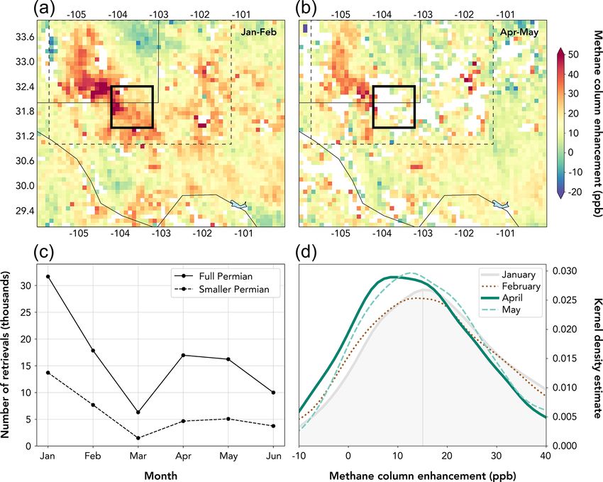
6606                                             D. R. Lyon et al.: Concurrent variation in methane emissions and oil price

top-down atmospheric measurements, primarily due to ab-
normal emissions that are difficult to quantify with bottom-
up approaches (Allen, 2014; Brandt et al., 2014; Zavala-
Araiza et al., 2017).
   The Permian Basin (Fig. 1) is the most productive oil
basin in the USA and rivals the Ghawar Field in Saudi Ara-
bia for the global record (Jacobs, 2019). Although the first
oil well was drilled in the Permian Basin nearly 100 years
ago, the basin has experienced rapid growth in recent years
as directional drilling and hydraulic fracturing allowed for
production from unconventional reservoirs (Enverus, 2021).
In 2019, the Permian Basin had ∼ 600 new wells drilled
per month and produced an average of 4.3 million barrels
(bbl) (6.8 × 10⁸ L) of oil and 15 billion cubic feet (Bcf)
(4.2 × 10⁸ m3 ) of natural gas per day, more than double the
2016 average values (Enverus, 2021). The Permian Basin’s
limited midstream infrastructure for delivering natural gas to
market results in high rates of associated gas flaring relative
to other US basins. In 2019, average daily flared gas volumes
were 0.8 Bcf (2.3 × 10⁷ m3 ), which is 5 % of the basin’s nat-    Figure 1. Regional map with outlines of the Permian Basin (or-
ural gas production (Appendix A). There is limited methane        ange), Delaware and Midland subbasins (dashed green and pur-
emissions data from the Permian Basin beyond two recent           ple), and the 100 km × 100 km study area (black). Locations of
studies (Zhang et al., 2020; Robertson et al., 2020). Zhang       the methane measurement tower sites are shown with red stars. A
et al. (2020) used satellite observations from May 2018–          heatmap displays combined natural gas and oil production from
                                                                  2019 expressed in barrel-of-oil equivalent (BOE) and gridded to
March 2019 in an atmospheric inversion to estimate total
                                                                  0.1◦ × 0.1◦ resolution (Enverus, 2021). Map was generated in Ar-
O&G-related emissions in the Permian Basin of 2.7 Tg CH4          cGIS Pro with imagery provided by Esri, Garmin, FAO, NOAA, and
annually or 3.7 % of regional gas production. Robertson et        USGS.
al. (2020) found higher well pad CH4 emission rates in the
Permian Basin compared to most other US basins based on
over 70 site-level measurements made in 2018. Alvarez et
al. (2018), which predates these studies, had assumed other       commodity prices reduce investment in new well and in-
US basins were representative of the Permian; updating their      frastructure development; in the Permian Basin, the number
estimate with the Permian Basin loss rate from Zhang et           of active drilling rigs, which had averaged over 400 from
al. (2020) results in a roughly 10 % increase in the US supply    April 2019 to March 2020, dropped below 200 by early May
chain estimate to 14.2 Tg CH4 or 2.5 % of total gas produc-       and reached a minimum of 123 in September (Baker-Hughes,
tion.                                                             2020) (Fig. 2).
   In January 2020, oil prices declined as the COVID-19 pan-         We hypothesize that the rapid drop in oil price would be
demic triggered a global slowdown in oil and natural gas          affiliated with a concomitant reduction in methane emissions
consumption; in March 2020, there was a rapid price drop          due to lower rates of well development and a subsequent
when the oil oversupply was exacerbated by both the Orga-         decline in oil and natural gas production. The postulated
nization of the Petroleum Exporting Countries (OPEC) fail-        causal mechanism for this relationship is the effect of asso-
ing to reach a deal to cut production and global oil storage      ciated natural gas production from new wells on midstream
capacity reaching its limit (Reed and Krauss, 2020). Spot         infrastructure throughput. During periods of higher commod-
prices for the US oil benchmark, known as West Texas In-          ity prices, the rapid growth in natural gas production likely
termediate – Cushing (WTI-Cushing), varied dramatically           exceeds the capacity of the midstream pipelines, compres-
during this period; price per barrel was relatively stable at     sor stations, and processing plants that deliver natural gas to
USD 50–60 for most of 2019, declined to USD 20 by late            market, leading to associated gas flaring and anomalous con-
April 2020, briefly dropped below zero on 20 April, and           ditions such as over-pressurization that increase emissions.
then recovered to USD 40 by early July (USEIA, 2020b).            Such trends were observed in an earlier drilling slowdown in
Natural gas spot prices (Henry Hub) were less volatile dur-       the Bakken region, another US unconventional oil formation
ing this period (USD 1.50–2.00 per million British Ther-          (Enverus, 2021) (Fig. F1). However, this effect might have
mal Units), continuing a gradual downward trend since late        been countered in the Permian Basin if lower profit mar-
2018 (USEIA, 2020a). In the Permian Basin, oil price is a         gins led operators to allocate fewer resources to infrastruc-
stronger driver of well development than natural gas price        ture maintenance and emissions mitigation, or similarly, re-
since many operators view oil as the primary product. Lower       strictions due to COVID-19 reduced the number of field staff

Atmos. Chem. Phys., 21, 6605–6626, 2021                                             https://doi.org/10.5194/acp-21-6605-2021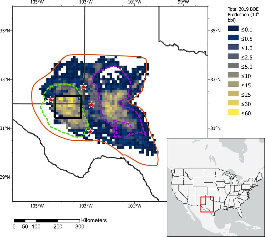
D. R. Lyon et al.: Concurrent variation in methane emissions and oil price                                                       6607

                                                                        atmospheric boundary layer (ABL) methane concentration
                                                                        ([CH4 ]) along the study area perimeter during six daytime
                                                                        flights (22 January, 9 March, 25 March, 4 May, 21 May,
                                                                        and 13 July; Sect. 2.2.2). The second approach continuously
                                                                        quantified [CH4 ] from March through August 2020 using
                                                                        sensors installed at three tall towers and one mountaintop sta-
                                                                        tion located around the perimeter of the study area (Richard-
                                                                        son et al., 2017; Sect. 2.2.1). Both approaches estimated
                                                                        study area methane flux on a daily basis by optimizing a prior
                                                                        emissions inventory to minimize model–data differences be-
                                                                        tween observed and simulated regional atmospheric [CH4 ]
                                                                        (Barkley et al., 2017; Sect. 2.2.1 and 2.2.3).
                                                                           We also evaluated satellite-based remote sensing obser-
                                                                        vations of column methane enhancement (1XCH4 ) for ev-
                                                                        idence of basin-wide trends (Sect. 2.2.4). To provide insights
                                                                        about the contribution of natural gas flares to methane emis-
                                                                        sions, we qualitatively assessed over 300 flares across the
Figure 2. Weekly count of active drilling rigs by type in the Permian   basin in February, March, and June 2020 using helicopter-
Basin between July 2019 and August 2020 (Baker Hughes, 2020).
                                                                        based infrared optical gas imaging (OGI) to visually detect
                                                                        the prevalence of unlit flares and combustion issues (Lyon et
                                                                        al., 2016; Appendix B). We estimated flare-related methane
performing tasks such as leak detection and repair (LDAR)
                                                                        emissions by applying combustion efficiency assumptions
(Gould et al., 2020).
                                                                        based on survey results to flared gas volume estimates based
                                                                        on satellite observations of flare radiant heat by the Visible
                                                                        Infrared Imaging Radiometer Suite (VIIRS) (Elvidge et al.,
2     Study area and methods
                                                                        2016; Appendix A).
2.1    Study area description
                                                                        2.2.1   Regional atmospheric [CH4 ] reanalysis
In January 2020, we began quantifying O&G methane emis-
sions at varying spatiotemporal scales within the Permian               An atmospheric reanalysis similar to the system used in
Basin with a concentrated effort within a 100 km × 100 km               previous studies (Barkley et al., 2019, 2017) was used
area of the Delaware subbasin along the Texas–New Mexico                to create simulated regional atmospheric [CH4 ] estimates.
border (Fig. 1). The 10 000 km2 study area includes ∼ 11 000            The modeling system used the Weather Research and
active wells and accounts for 33 % and 43 % of the Per-                 Forecasting (WRF) model coupled with chemistry (WRF-
mian Basin’s oil and natural gas production in 2019, re-                Chem v3.6) (Skamarock et al., 2008) configured to sim-
spectively (Enverus, 2021). The study area has a high den-              ulate two domains, an outer 2600 km × 2100 km domain
sity of midstream O&G infrastructure including at least 125             with 9 km × 9 km horizontal resolution and 50 vertical lev-
gathering and transmission compressor stations, 44 process-             els, with about 30 of these levels in the lowest 3 km above
ing plants, and ∼ 32 000 km of gathering pipeline (Enverus,             ground level, and an inner 830 km × 830 km domain with
2021). Based on spatially allocated USEPA inventory data,               3 km × 3 km horizontal resolution and the same vertical lay-
O&G sources accounted for > 90 % of methane emissions                   ers. The outer domain is nudged to ERA5 wind, temper-
in the study area in 2012; other sources, dominated by agri-            ature and water vapor reanalyses, and the inner domain
culture and waste, were responsible for ∼ 0.5 Mg CH4 h−1                is nudged to regional observations including ∼ 50 US Na-
(Maasakkers et al., 2016). Since the non-O&G sources ac-                tional Weather Service and World Meteorological Organiza-
count for only a small fraction of total emissions and there            tion (WMO) surface stations, five National Weather Service
have been no major changes in these activities over the past            rawinsonde site soundings launched at 00:00 and 12:00 UTC,
few years, we have assumed all study area emissions are at-             and the meteorological measurements from commercial air-
tributable to O&G sources beyond the 0.5 Mg CH4 h−1 .                   craft. Our choice of parameterization schemes within WRF-
                                                                        Chem matches previous studies (Barkley et al., 2019, 2017).
2.2    Method overview                                                     Only atmospheric [CH4 ] from emissions within the model
                                                                        domain are simulated, using techniques demonstrated previ-
Between January and August 2020, we used two inver-                     ously (Barkley et al., 2019, 2017). Preliminary estimates of
sion approaches to quantify total methane emission flux                 surface fluxes of [CH4 ] within the domain are taken from the
from the study area at a weekly to monthly frequency. The               USEPA 2012 gridded inventory (Maasakkers et al., 2016),
first approach used aircraft-based instruments to measure               save for the Permian Basin where an updated, production-

https://doi.org/10.5194/acp-21-6605-2021                                                 Atmos. Chem. Phys., 21, 6605–6626, 2021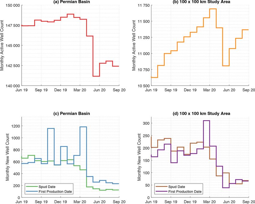
6608                                              D. R. Lyon et al.: Concurrent variation in methane emissions and oil price

based inventory is used. This updated inventory is described       computation of horizontal wind speeds and directions; and a
in detail by Zhang et al. (2020). Briefly, production site CH4     Vaisala probe to measure ambient temperature and relative
emission factors were developed using methods in Zavala-           humidity (RH).
Araiza et al. (2015) and based on measurements by Robert-             On each flight day, two laps consisting of a box enclosing
son et al. (2020), which accounted for complexity of well site     the 100 km × 100 km study area were flown at 335 ± 30 m
infrastructure and their related CH4 emissions. Total basin-       above ground level (a.g.l.), with one complete lap taking
wide CH4 emissions were estimated using activity (Enverus,         ∼ 2 h to complete. Two to three vertical profiles were also
2021) and disaggregated to individual sites based on their gas     flown by the aircraft as pairs of ascents and descents between
production. Additional facility-level CH4 emissions for gath-      the lowest safe flight altitude (typically 61 to 152 m a.g.l.)
ering and boosting stations, gathering pipelines, and process-     and the flight altitude at which significant changes are ob-
ing plants were estimated based on activity data (Enverus,         served in measured species concentrations (e.g., CH4 , water
2021) as well as CH4 emission factors from Marchese et             vapor, relative humidity, and potential temperature) – typi-
al. (2015) and the USEPA GHGI (USEPA, 2020a). For the              cally 914 to 3048 m a.g.l. Plots of a.g.l. altitude versus these
transmission and storage stations, CH4 emissions were taken        species are used to assess the mixing height of surface emis-
from Maasakkers et al. (2016). For the Delaware subbasin,          sions. Both CH4 concentrations along the flight path and the
total CH4 emissions were estimated at 1.2, 0.11, 0.04, and         mixing height determined from the airborne vertical profiles
0.01 Tg for production sites, gathering and boosting stations,     are used in transport modeling to determine emissions from
gas processing plants, and gas transmission and distribution       the entire study area.
stations, respectively. These point-source oil and natural gas        [CH4 ] emissions are computed from each complete cir-
CH4 emissions were then spatially allocated to a 0.1◦ × 0.1◦       cuit of the study area by the aircraft. This is done by com-
grid over the entire basin. This update within the Delaware        paring the observed and simulated [CH4 ] enhancement, the
subbasin is important to account for the rapid development         increase in [CH4 ] downwind of the study area relative to a
within the basin since 2012. Different [CH4 ] sources (e.g., oil   background value, and adjusting emissions within the study
and natural gas production, landfills, agriculture) and sources    area to minimize the absolute error between the simulated
inside and outside the study domain are tagged as indepen-         and observed atmospheric boundary layer [CH4 ]. The 10th
dent tracers in the model. Oil and gas emissions outside of        percentile of [CH4 ] observations in the circuit determines
the study domain are multiplied by 1.6 to match estimates          the background. This mole fraction value is subtracted from
from Alvarez et al. (2018) and to better account for develop-      the observed [CH4 ] observations, resulting in an estimate of
ment in the areas surrounding the study domain. This atmo-         [CH4 ] enhancements. These observed enhancements are then
spheric reanalysis system enables us to create a first estimate    compared to simulated [CH4 ] enhancements by matching ob-
of atmospheric [CH4 ] consistent with the regional meteorol-       servation and model at the nearest grid points in space and
ogy and the preliminary estimate of sources within the outer       time. Simulated enhancements are split into two categories:
model domain.                                                      study domain enhancements and enhancements originating
   Note that the emissions magnitude from the preliminary          from outside the study domain. Enhancements associated
[CH4 ] emissions estimates is not highly important since the       with sources outside the study domain are subtracted from
emissions estimate is not a Bayesian inversion that assigns an     the observed [CH4 ] enhancements, resulting in a set of ob-
uncertainty estimate to this preliminary estimate. The spatial     servations whose enhancements can be directly attributed to
pattern of emissions, however, including the relative change       emissions within the study domain. The simulated study do-
in these spatial patterns, is important for the estimate of        main enhancements are then compared to the observed study
fluxes. Our assumption that emissions are proportional to gas      domain enhancement, and a scalar multiplier is applied to the
production should provide a reasonable estimate of the spa-        simulated enhancements to minimize the absolute error be-
tial pattern of emissions corresponding to the location of oil     tween the two datasets. Because the emissions scale linearly
and natural gas infrastructure (Maasakkers et al., 2016).          with the simulated enhancements, this scalar multiplier, ap-
                                                                   plied to the preliminary emissions estimate within the study
2.2.2   Aircraft-based methane emission estimates                  area, provides a solution to the emissions within the study
                                                                   domain (Barkley et al., 2017). The solution for each circuit
The total CH4 emissions in the Permian Basin study area            is merged into a single daily estimate.
were determined using airborne data in conjunction with               To test the uncertainty of the emission rate solution for
transport modeling. The airborne platform has been deployed        each flight day, a 1000-iteration Monte Carlo uncertainty as-
and described previously (Conley et al., 2017, 2016; Kar-          sessment was performed, adjusting various parameters to test
ion et al., 2015; Smith et al., 2017). In brief, a single-         how they impacted the solution. Through the iterations, we
engine Mooney aircraft is outfitted with a Picarro cavity ring-    examine the impact of various possible sources of error, in-
down spectrometer (CRDS) instrument (G2210-m) to mea-              cluding uncertainty in the background, uncertainty in the as-
sure in situ atmospheric CH4 , CO2 , and H2 O mole frac-           sumed influence from sources outside the domain, and un-
tions; a differential GPS and aircraft data computer to enable     certainty in the atmospheric transport. For uncertainty in the

Atmos. Chem. Phys., 21, 6605–6626, 2021                                              https://doi.org/10.5194/acp-21-6605-2021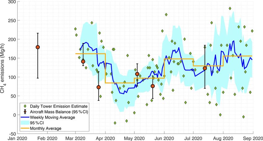
D. R. Lyon et al.: Concurrent variation in methane emissions and oil price 6609
ment uncertainty values (including instrument noise, uncer-
tainty due to water vapor calibration, and tank assignment
uncertainty) for the four tower locations were 0.6 ppb (Carls-
bad), 0.6 ppb (Fort Stockton), 3.4 ppb (Hobbs), and 5.4 ppb
(Notrees), with the differences being attributable to different
instrument types: short Nafion dryer in the case of Hobbs and
laser aging for Notrees.
CH4 emissions in the study domain were calculated for
each day of tower observations using a similar technique as
used with the aircraft observations. Daily afternoon [CH4 ]
at each tower site averaged from 16:00–22:00 UTC (11:00–
17:00 local standard time) was computed from both the ob-
servations and the simulation. A background [CH4 ] value
(both for the observations and the model) is selected based
on the lowest measurement from the available tower sites.
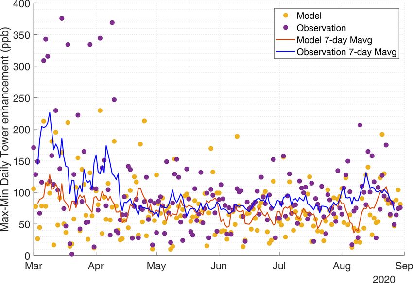
Figure 3. Comparison between modeled and observed differences This background is subtracted from all tower sites to create
in the maximum and minimum daily CH4 enhancement across the an observed [CH4 ] enhancement. Simulated enhancements
tower network. Also shown are the 7 d moving averages (Mavg) of from sources outside of the domain are subtracted from the
each trend.
observed enhancements to produce an observed [CH4 ] en-
hancement associated with sources inside the study domain.
background, we select a random percentile between the 5th A scalar multiplier is then applied to minimize the absolute
and 15th to use as the methane background in a flight lap. For error between the observed and modeled enhancements, and
uncertainty in sources outside of the domain that are sub- a daily emission rate is solved for in the study domain.
tracted from the observations, we multiply the “other” en- Unlike the aircraft mass balance observations, which are
hancement tracer by a random factor between 0.5 and 1.5 to collected on days when meteorological conditions are ideal
account for the possibility that regional emissions may be in- for measuring emissions from the study domain, the tower
correct. For uncertainty in the transport, the time of the obser- dataset is continuous, and many days may not be suitable for
vations is adjusted by ±30 min, creating perturbations to the calculating an emission rate from the study domain. The most
model output timeframe used to compare to the observations. useful tower observations for solving for emissions within
From the 1000 iterations, the 2.5th and 97.5th percentiles of the study domain are those whose enhancements are influ-
solutions are chosen to represent the 95 % confidence inter- enced primarily by sources within the study domain and con-
val. tain minimal enhancements from sources outside of the do-
main. We select for these conditions by retaining days when
2.2.3 Tower-based methane emissions estimates > 50 % of the simulated downwind afternoon tower enhance-
ments come from sources within the study domain. This fil-
Atmospheric mole fraction measurements of CH4 and CO2 tering removes 85 of 184 available days, most of which have
were collected at five locations in the Permian Basin begin- easterly winds and contain air masses heavily influenced by
ning 1 March 2020, using methods similar to those described the Midland subbasin to the east as well as oil and gas basins
in Richardson et al. (2017). A map of the measurement loca- in central and eastern Texas. For the remaining 99 d, we
tions, along with oil and gas facilities in the Permian Basin, is remove 4 d whose solutions are more than 3 median abso-
shown in Fig. 1. Note that only four of the five planned mea- lute deviations away from the median solution, presumably
surement sites are used in this analysis and shown in Fig. 1 caused by issues in the model transport; excluding these out-
due to instrument malfunctions at the northernmost site. Of lier days has a minor impact on overall results. In total, 95 d
these measurement locations, three were on towers at mea- is used to calculate emissions and trends in the tower dataset
surement heights of 91–134 m a.g.l., and the westernmost between 1 March and 30 August 2020.
site was at a mountaintop station on a rooftop 4 m a.g.l. The
measurements were made with wavelength-scanned cavity 2.2.4 TROPOMI-derived column-averaged methane
ring-down spectroscopic instruments (Picarro, Inc., models mixing ratios
G2301, G2401, G2204, and G2132-i). The air samples were
dried using Nafion dryers (Perma Pure, Inc.) in reflux mode, We use column-averaged dry-air methane mixing ratios
with an internal water vapor correction applied for the effects (XCH4 ) from the TROPOspheric Monitoring Instrument
of the remaining water vapor (< 1 %). The instruments were (TROPOMI) from January to June 2020. TROPOMI was
calibrated in the laboratory prior to deployment and using launched in October 2017 aboard the polar sun-synchronous
quasi-daily field tanks traceable to the WMO X2004A scale Sentinel-5 Precursor satellite with an ∼ 13:30 local overpass
(Dlugokencky et al., 2005; NOAA, 2015). The CH4 measure- time. It provides daily global coverage with 7 km × 7 km
https://doi.org/10.5194/acp-21-6605-2021 Atmos. Chem. Phys., 21, 6605–6626, 2021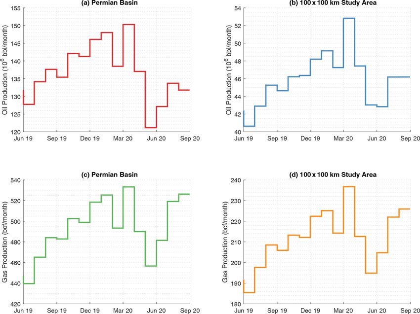
6610                                                 D. R. Lyon et al.: Concurrent variation in methane emissions and oil price

Figure 4. Tower and aerial emission estimates from the 100 km × 100 km study area through 31 August 2020. Individual daily accepted
estimates from the tower observations are shown in green diamonds, while red circles with error bars represent the aerial estimate and 95 %
CI (confidence interval) range. The blue line represents the 7-data-point moving average of the tower estimates and the light blue shading
shows the 95 % CI range expressed as twice the 7-data-point moving standard error. The orange line represents the monthly average estimate
from the combination of aerial and tower-based methods which weights tower and aircraft-based estimates equally.

Table 1. Numerical estimates of CH4 flux from the 100 km × 100 km study area derived from the combination of tower and aerial measure-
ments across several temporal ranges.

   Time range                              Mean emissions       Number of accepted daily     Standard deviation   Standard error            95 % CI
                                                (Mg h−1 )   measurements (tower, aircraft)           (Mg h−1 )        (Mg h−1 )    emission estimate
   Mar 2020                                          162                           (17, 2)                  67               15            131–193
   Apr 2020                                           84                           (14, 0)                  63               17             50–118
   May 2020                                           97                           (22, 2)                  47               10             78–116
   Jun 2020                                          148                           (18, 0)                  73               17            113–182
   Jul 2020                                          129                           (14, 1)                  93               24             82–177
   Aug 2020                                          156                           (16, 0)                  97               24            107–204
   “Pre-Crash Period” 22 Jan–19 Mar 2020             186                           (10, 2)                  59               17            152–220
   “Emissions Minima” 11 Apr–5 May 2020               65                           (13, 1)                  53               14              36–93

pixel resolution at nadir (Hu et al., 2018); the pixel reso-                TROPOMI observations are available per month across this
lution has changed to ∼ 7 km × 5.5 km at nadir since Au-                    domain, neglecting March and June (Fig. 5c). To mitigate the
gust 2019. The XCH4 retrieval uses sunlight backscattered                   impact of reduced spatial coverage on our change analysis
by the Earth’s surface and atmosphere in the shortwave in-                  after February, we manually discard observations from days
frared (SWIR) spectral range and has near-unit sensitiv-                    with little to no coverage of the Delaware and/or Midland
ity down to the surface (Hasekamp et al., 2019). Here we                    subbasins. Data from 20 %–40 % of observation days in Jan-
consider only higher-quality XCH4 measurements based on                     uary, February, April, and May (depending on the month) are
published quality assurance metrics (quality assurance value                discarded in this way, but the total number of observations is
> 0.5; Apituley et al., 2017).                                              reduced by only 5 %.
   We calculate the daily methane enhancements over the                        Repeating our analysis with the background defined at the
Permian Basin from topography-corrected XCH4 , relative to                  25th percentile level (rather than the 10th), we find that trends
a regional background column defined by the 10th percentile                 are insensitive to the percentile value used. Furthermore, the
of XCH4 across the full Permian Basin domain (29–34◦ N                      trends are not explained by seasonal changes in wind speed
and 100–106◦ W). The topography correction is based on                      across the Permian Basin. Higher winds could lead to lower
a linear regression of XCH4 against surface altitude (simi-                 enhancements, but data from the NASA GEOS-FP (Lucch-
lar to the methodology presented in Kort et al., 2014, and                  esi, 2013) meteorological reanalysis product indicate that the
Zhang et al., 2020, performed across the continental United                 daily wind speed averaged over the full Permian Basin do-
States (25–48◦ N and 66–125◦ W)). Roughly 5000–14 000                       main, in the lowest 3 km of the atmosphere, during the 6 h

Atmos. Chem. Phys., 21, 6605–6626, 2021                                                           https://doi.org/10.5194/acp-21-6605-2021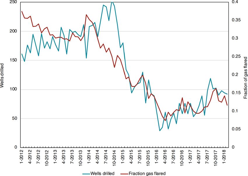
D. R. Lyon et al.: Concurrent variation in methane emissions and oil price                                                             6611

Figure 5. TROPOMI observations of topography-corrected methane column enhancements over the Permian Basin, from January to
June 2020. (a–b) Mean methane column enhancements (ppb) over the Permian Basin for the January–February and April–May 2020
time periods, gridded to 0.1◦ × 0.1◦ resolution. The thin solid lines indicate state and national borders; the thick solid lines describe the
100 km × 100 km tower and aircraft study region; and the dotted lines trace a smaller Permian Basin domain that closely bounds the methane
hotspots seen over the Delaware and Midland subbasins. (c) Number of TROPOMI column retrievals over the full Permian Basin domain
(29–34◦ N and 100–106◦ W) and over the smaller Permian Basin domain (31–34◦ N and 101.4–105.6◦ W; dashed lines in panels a, b) by
month in 2020. (d) Frequency distribution plots of methane column enhancements over the smaller Permian Basin domain by month, after
removal of days without coverage of the Delaware and/or Midland subbasins (see text). The gray vertical line indicates the distribution
maximum for January.

closest to TROPOMI observation time (15:00–21:00 UTC),                   behavior of local emissions. From the tower network, we
decreased from a mean of 7.02 m s−1 in January–February to               frequently observe large enhancements > 200 ppb in March
5.48 m s−1 in April–May.                                                 and mid-April, after which point the enhancement rarely
                                                                         increases above 150 ppb for the remainder of the summer
                                                                         months. It should be noted that a slight decrease in the size of
3     Results                                                            the enhancements would be expected during this period due
                                                                         to increased vertical mixing in a seasonally growing bound-
3.1    Tower and aircraft-based methane emissions
                                                                         ary layer; however, modeled results from this time span ex-
       estimates
                                                                         hibit a much smaller magnitude of change. Therefore, the
                                                                         dramatic decline in CH4 enhancements coincident with the
Figure 3 presents the daily difference between the high-
                                                                         timing of the price crash is likely due to a change in the emis-
est and lowest observed CH4 measurement across the tower
                                                                         sions rather than a change in the meteorology.
network. Although the overall magnitude of the study area
                                                                            Figure 4 presents a time series of CH4 emissions within
plume observed at the tower network can be affected by
                                                                         the 100 km × 100 km study area between 1 March and
various meteorological factors (e.g., wind speed, direction,
                                                                         31 August 2020 from both aircraft and tower-based ap-
boundary layer height), large changes in the typical size of
                                                                         proaches. The 95 % CI (confidence interval) ranges are de-
the observed plumes can be indicative of a sudden shift in

https://doi.org/10.5194/acp-21-6605-2021                                                   Atmos. Chem. Phys., 21, 6605–6626, 2021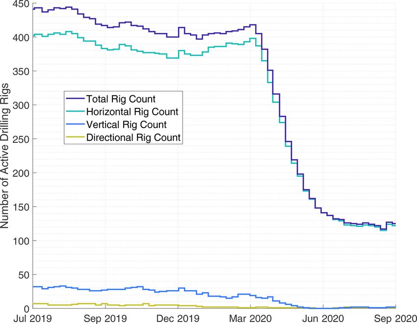
6612                                                   D. R. Lyon et al.: Concurrent variation in methane emissions and oil price

                                                                          Figure 8. VIIRS-derived gas flaring in the study region. (a) Spa-
                                                                          tial distribution of the cumulative adjusted radiant heat over the
Figure 6. Temporal variation in methane emissions and crude oil           period between January 2019 and June 2020 aggregated over a
price. (a) Aerial (red circles with 95 % CI error range) and tower-       0.05◦ × 0.05◦ grid resolution. (b) Histogram of VIIRS-derived
based 7-point moving average and 95 % CI (blue line and shad-             source temperatures. Dotted lines show the temperature regime
ing) atmospheric estimates of 100 km × 100 km study area CH4              characteristic of gas flaring sources (1400—2500 K). (c) Monthly
emissions. (b) 7 d moving average of WTI-Cushing daily oil price.         trend in VIIRS-derived gas flared volumes. The mean estimate is
(c) Orange line and shading presents resulting CH4 loss rate com-         shown with a solid line, and the 95 % CI on the mean is shown in
bined aerial and tower-based measurements utilizing published             the shaded area. 1 billion cubic feet (Bcf) = 2.8 × 10⁷ m3
monthly gas production within the study area (Enverus, 2021). Red
points present the loss rate utilizing only the aircraft-based emission
estimates and the monthly gas production during the month of the
flight.
                                                                          rived from twice the standard error of all accepted daily
                                                                          tower-based estimates in each month. Both aircraft and
                                                                          tower-based methane flux data show consistent trends of de-
                                                                          clining then rebounding methane emissions in our Permian
                                                                          Basin study area. Between 22 January and 19 March 2020,
                                                                          emissions were 186 Mg CH4 h−1 (95 % confidence interval
                                                                          range: 152–220 Mg CH4 h−1 ). Following the rapid decrease
                                                                          in oil price, emissions between 11 April and 5 May 2020
                                                                          reached a minimum of 65 Mg CH4 h−1 (95 % CI range:
                                                                          36–93 Mg CH4 h−1 ). After the oil price partially recov-
                                                                          ered, emissions for the month of June had increased to
                                                                          148 Mg CH4 h−1 (95 % CI range 113–182 Mg CH4 h−1 ).
                                                                          Mean emission estimates for the remainder of the summer
                                                                          months were slightly below those before the crash, although
                                                                          show much higher uncertainty due to increased difficulty in
                                                                          resolving the signal of emissions from within and outside of
                                                                          the study area boundary due to increasing mixing depths and
                                                                          thus a dilution of the signal.
Figure 7. Number of new well pads constructed per month be-                  Combining the monthly tower and aircraft-based estimates
tween 1 August 2019 and 31 July 2020 in the full Permian Basin            with reported gas production (Enverus, 2021), we calculate a
and our 10 000 km2 Delaware subbasin study area based on satellite        March 2020 loss rate of 3.3 % of total gas production (95 %
imagery and machine learning (Appendix C).                                CI range: 2.7 %–4.0 %), which is slightly lower but within
                                                                          the uncertainty of previously reported basin-wide estimates

Atmos. Chem. Phys., 21, 6605–6626, 2021                                                     https://doi.org/10.5194/acp-21-6605-2021
D. R. Lyon et al.: Concurrent variation in methane emissions and oil price                                               6613

from 2018–2019 (3.7 ± 0.7 (1σ ) %) (Zhang et al., 2020). The    3.3    Emission contribution from flaring and well
minimum loss rate calculated for April 2020 was 1.9 % of gas           completions
production (95 % CI range: 1.1 %–2.6 %), increasing gradu-
ally for the summer months to again exceed 3.0 %.               Well pad development in the study area proceeded at an av-
                                                                erage rate of 71 new sites per month between August 2019
3.2   TROPOMI-derived column-averaged methane                   and March 2020 and then dropped to a monthly average of 24
      mixing ratios                                             sites between April and July 2020 (Appendix C, Fig. 7). The
                                                                number of well completions per month declined from 188 to
In the full Permian Basin, orbital observations of XCH4 indi-   115 between January and April 2020 (Enverus, 2021); com-
cate lower methane column enhancements in April–May ver-        pletion counts are higher than well pad development rates
sus January–February 2020, consistent with the aircraft and     due to multiple wells being located on a single pad. After ris-
tower-based flux data (Fig. 5). Figure 5a and b show mean       ing steadily throughout 2019, oil and gas production peaked
methane column enhancements over the Permian Basin, ob-         in March 2020 and then declined 9 % and 8 %, respectively,
served by TROPOMI in (a) January–February 2020 and              in April. Based on adjusted, incomplete production data for
(b) April–May 2020. Enhancements over the Permian Basin         May and June, gas production stayed relatively steady after
appear to be lower in April–May compared to January–            April, while oil production dropped an additional 3 % (Ap-
February, as indicated by an ∼ 18 % reduction in the re-        pendix E). The relative decline in oil and natural gas produc-
gional mean between those two periods. This reduction           tion between March and April 2020 was much greater among
may be due in part to lower spatial coverage after Febru-       wells in the first 2 months of production, decreasing 50 % and
ary 2020, likely caused by the introduction in March of a       45 %, for oil and gas, respectively (Appendix E).
different cloud mask product in the TROPOMI retrieval al-          The three flare surveys between February and June 2020
gorithm (Siddans, 2020). Considering TROPOMI retrievals         consistently found that 11 % of flares had combustion is-
with quality assurance values of 0.5 or greater, we obtain      sues, with 5 % unlit and emitting hydrocarbons. Even when
roughly 6000–32 000 enhancement measurements per month          using conservative assumptions of higher combustion effi-
from January to June 2020 over the full Permian Basin           ciency, we estimate a basin-wide flare combustion efficiency
(Fig. 5c). The limited number of satellite observations over    of 93 %, with the remaining gas (assuming 80 % methane
our 100 km × 100 km study area for tower and aircraft mea-      content) being emitted to the atmosphere (Appendix B).
surements (Fig. 3) precludes direct comparison with the sub-    Satellite observations of radiant heat indicate that flared gas
orbital measurements; therefore, we provide here an analysis    volumes were cut in half from 7.6 to 3.2 Bcf (2.2 × 10⁸ to
of TROPOMI methane enhancement over the broader Per-            9.1 × 10⁷ m3 ) between January and April 2020 (Fig. 8).
mian Basin. Coverage is particularly sparse in March and
June, so we neglect those 2 months in the TROPOMI analy-
sis presented here.                                             4     Discussion
   Figure 5d shows frequency distributions of methane col-
umn enhancements observed by TROPOMI in January,                The pandemic-associated oil price crash provided an unex-
February, April, and May 2020. For these monthly curves, we     pected opportunity to assess temporal variability in methane
restrict our attention to a smaller Permian Basin domain that   emissions during a period of volatile oil prices and associ-
closely bounds the methane hotspots seen over the Delaware      ated operational changes. In support of our hypothesis that
and Midland subbasins (dashed lines in Fig. 5a, b; 31–34◦ N     methane emissions would decline with oil price, we observed
and 101.4–105.6◦ W). Permian Basin methane enhancements         a threefold reduction in Permian Basin study area methane
as observed by TROPOMI appear to decrease in early 2020,        emissions that was strongly correlated to the average daily oil
reaching a minimum in April before beginning to rise again      price. Between Q1 and Q2 2020, Permian Basin oil and natu-
in May. The trends we identify in TROPOMI methane en-           ral gas production dropped about 12 % and 8 % respectively;
hancement analysis across the Permian Basin are broadly         the magnitude of change for oil and gas production was
consistent with our findings from tower and aircraft obser-     similarly about 11 % and 9 % within the 100 km × 100 km
vations of reduced emissions particularly during April in our   study area (Fig. E1). Accordingly, the loss rate temporar-
campaign domain of the Delaware subbasin, but large uncer-      ily decreased from 3.3 % to 1.9 % of gas production be-
tainties remain due to the different spatial domains and the    tween 22 January–19 March and 11 April–5 May 2020 (Ap-
reduced satellite coverage after February 2020. More data       pendix E). It is important to note that even the minimum
and/or more advanced analysis using inverse modeling tech-      observed loss rate of 1.9 % is several times higher than the
niques may be needed to reliably characterize Permian Basin     performance targets committed to by major oil and natu-
methane emission trends using TROPOMI satellite observa-        ral gas production companies accounting for about one-third
tions.                                                          of global oil production, including some with operations in
                                                                the Permian Basin (OGCI, 2020). We hypothesize that to-
                                                                tal methane emissions are positively correlated with oil price

https://doi.org/10.5194/acp-21-6605-2021                                           Atmos. Chem. Phys., 21, 6605–6626, 2021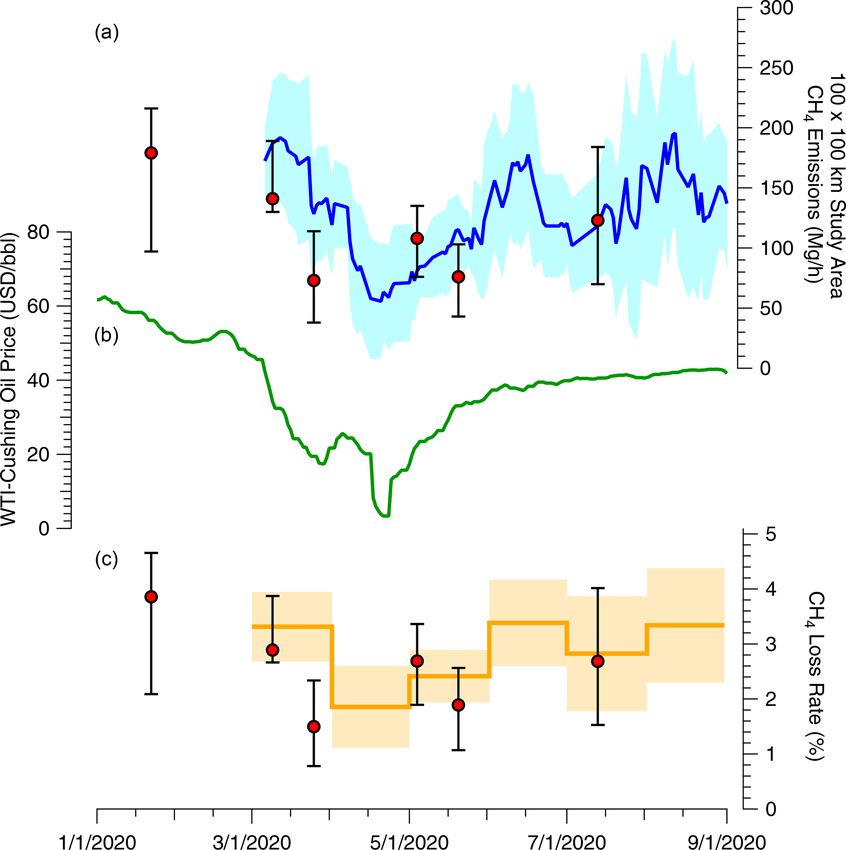
6614                                              D. R. Lyon et al.: Concurrent variation in methane emissions and oil price

due to three interrelated factors associated with well devel-      decrease in drilling and flaring rates (Appendix F). Our study
opment: (1) well completion rates, (2) associated gas flaring      provides the first direct evidence of reduced methane emis-
volumes, and (3) indirect impacts of new associated gas pro-       sions resulting from an apparent abatement of infrastructure
duction on the gathering and processing system.                    capacity limitations.
    Lower oil prices directly led to reduced emissions by de-         The high methane emission rate observed in the Permian
creasing well development activities, as we observed for rig       Basin during periods of higher oil commodity prices is likely
count, new site construction, and well completions follow-         a consequence of associated gas production increasing at a
ing the price crash. Well development activities are an inter-     faster rate than midstream infrastructure capacity for send-
mittent source of methane emissions, particularly completion       ing gas downstream. This leads to both intentional flaring
flowback, the typically multiday period following hydraulic        of stranded gas and fugitive emissions from anomalous con-
fracturing when fluids, excess proppant, and entrained gas         ditions related to excess gas throughput (e.g., pressure re-
are expelled from the wellbore (Allen et al., 2013). We es-        lief venting). Our observations of emissions declining con-
timate that the ∼ 70 fewer well completions in April versus        currently with new well development suggest that methane
January 2020 caused average potential flowback emissions           emissions could be mitigated in the Permian Basin and simi-
in our study area to decline from 45 to 26 Mg CH4 h−1 (Ap-         lar oil-producing fields by better aligning development rates
pendix D). At the time of the study, US federal regulations        of wells and midstream infrastructure. For example, regula-
mandated the use of reduced emission completions to con-           tions could prohibit the drilling of wells in areas without suf-
trol emissions in most situations; operator reported data sug-     ficient capacity to transport newly produced associated gas
gest actual emissions (2–4 Mg CH4 h−1 ) are less than 10 %         to market. Our findings suggest that policies which tie the
of potential emissions (USEPA, 2019, 2020b; Appendix D).           maximum rate of well development to infrastructure capac-
    The observed twofold reduction in flared gas volumes be-       ity, in addition to other approaches such as requiring high-
tween January and April 2020 was likely the result of the          frequency or continuous monitoring to detect large emission
large drop in associated gas production from new wells.            sources (Alvarez et al., 2018), can facilitate lower methane
Unconventional wells tend to have high initial gas produc-         emissions that reduce the climatic impact of oil and gas pro-
tion followed by steep declines. With lower rates of well          duction.
development and new gas production in the area, compe-
tition for limited gas pipeline capacity likely was abated,
leading to less flaring of stranded associated gas. Assuming
a combustion efficiency of 93 %, we estimate flare-related
methane emissions in our study area were approximately 8
and 3 Mg CH4 h−1 in January and April 2020, respectively
(Appendix A). Our combustion efficiency assumption, which
is based on repeat observations of over 300 flares, is conser-
vatively high; therefore, our emission estimate represents a
lower bound. However, even with worst-case assumptions of
flare combustion efficiency, it is unlikely that January and
April flare-related emissions would have exceeded 20 and
7 Mg CH4 h−1 , respectively (Appendix B).
    Our estimates of well completion and flare-related
methane emissions account for less than 20 % of the ob-
served total reduction between pre-crash and minimum price
conditions; therefore, we theorize that the primary driver of
emission reductions is indirect improvements to the perfor-
mance of the midstream gathering and processing system re-
sulting from reduced inputs of gas from new wells. This re-
sult suggests that the high methane emission rate observed in
the Permian Basin in recent years is in large part due to in-
sufficient capacity of midstream infrastructure for handling
and delivering rapidly growing rates of natural gas produc-
tion (Zhang et al., 2020). The drastic decline in flared associ-
ated gas volumes during the oil price crash suggests that the
reduction in new gas production relieved midstream capacity
issues. A similar pattern was observed in the Bakken forma-
tion during the oil price decline of 2015–2016: price drops
caused only a small decrease in total production but a large

Atmos. Chem. Phys., 21, 6605–6626, 2021                                              https://doi.org/10.5194/acp-21-6605-2021
D. R. Lyon et al.: Concurrent variation in methane emissions and oil price 6615
Appendix A: VIIRS-derived flared natural gas volumes were a factor of 2.6 and 2.8 times lower than the monthly
mean observed in 2019 for the 100 km × 100 km study re-
We assess the monthly trends in the volumes of natural gion and full Permian Basin, respectively.
gas flared in the study region using nighttime fire and flare
data observed by the Visible Infrared Imaging Radiometer
Suite (VIIRS) instrument aboard the Suomi National Polar- Appendix B: Aerial flare performance survey
orbiting Partnership satellite. Specifically, we use the VIIRS
NightFire V3.0 data product to support our analysis (Elvidge We compiled a list of potential locations of recently active
et al., 2013) For the study region and for the period be- flares in the Permian Basin (Delaware and Midland sub-
tween January 2019 and June 2020, we retrieved 49 885 in- basins) based on a geospatial analysis of the SkyTruth Global
dividual VIIRS detections for which it was possible to esti- Flaring Dataset, which is derived from heat sources detected
mate flaring source temperatures based on Planck curve fit- by the Visible Infrared Imaging Radiometer Suite (VIIRS)
ting of the source radiances (Elvidge et al., 2013). During instrument on the NOAA Suomi NPP satellite; SkyTruth
this period, the mean VIIRS-derived source temperature was has applied several filters to the VIIRS data including re-
1869 K. The histogram of source temperatures is shown in moving heat sources < 1500 ◦ C and with < 3 detections per
Fig. 8b, indicating a strong gas flaring signal in the char- month (Skytruth, 2020). To account for spatial uncertainty of
acteristic temperature regime of between 1400 and 2500 K. SkyTruth flare locations, we spatially joined their individual
Elvidge et al. (2015) developed a correlation between the flare detections between 1 October 2019 and 31 January 2020
VIIRS-derived radiant heat and reported gas flared volumes using a 100 m buffer distance; the centroid latitude and lon-
and derived the relationship: gitude of the 1014 joined detections were defined as likely
locations of recently active flares. Leak Surveys, Inc. (LSI),
Va = 0.0274 RH0 (R 2 = 0.86), (A1) a leak detection company specializing in aerial optical gas
where Va is the annual volume of gas flared (in billion cu- imaging, was provided a list of 573 potential active flare loca-
bic meters) and RH0 is the modified radiant heat for each tions from the original set of 1014. The site selection method-
individual flare, adjusted to account for the observed nonlin- ology balanced representativeness and survey efficiency by
ear relationship between flared gas volume and radiant heat defining one contiguous, high flare density area in each sub-
and was computed as RH0 = σ T 4 S 0.7 , where σ is the Stefan- basin that could be surveyed over the course of approxi-
Boltzmann constant (5.67 × 10⁻⁸ W m−2 K−1 ), T and S are mately 5 d. For the Delaware subbasin, we selected 323 lo-
the source temperature and area, respectively, and the expo- cations located within our main study area (NW and SE cor-
nent (0.7) was empirically developed by Elvidge et al. (2015) ners are 32.325◦ N, 103.822◦ W and 31.417◦ N, 103.202◦ W,
to address nonlinearity. Figure 8a shows the spatial distribu- respectively). For the Midland subbasin, we selected 250 lo-
tion of the cumulative RH0 in the study region over the period cations from the two counties (Midland and Martin) with the
between January 2019 and June 2020, as aggregated over a highest flare counts from the analysis of VIIRS data. LSI
0.05◦ × 0.05◦ grid resolution. To estimate monthly gas flared surveyed these locations with a custom infrared camera (IR)
volumes (Vm in billion cubic feet) for the study area, we mod- deployed in a R44 helicopter. Potential flare locations were
ify the equation above, assuming the relationship holds over identified with spatial coordinates and a unique flare ID.
monthly intervals: LSI performed three surveys of the potential flare lo-
cations during the weeks of 17 February, 23 March, and
Vm = 0.0274RH0 × f/12 (A2) 22 June 2020 (EDF, 2020). At each potential flare location,
LSI determined if one or more flares was present at the spa-
where f is the conversion between cubic meters and cubic tial coordinates, and if so, it observed the flare(s) for oper-
feet (1 m3 = 35.315 ft3 ). We use the equation above to com- ational status. For flares with apparent combustion issues,
pute the mean monthly gas flared volumes (and 95 % CI on LSI recorded 30–60 s of infrared and visual video footage
the mean) in the study area based on the daily RH0 aggregated of the flare plume to provide visual evidence of flare status.
from individual detected flares. The trend in the monthly gas For each flare, LSI assigned a qualitative assessment of the
flared volumes is shown in Fig. 8c. The average flaring rate apparent flare status at the time of survey from four cate-
in 2019 was 8.2±2.2 Bcf month−1 (2.3×10⁸ ±6.2×10⁷ m3 ). gories: inactive and unlit with no emissions (inactive); ac-
From February 2020, a sharp decline in the mean gas flaring tive, lit, and operating properly (operational); active and lit
rate was observed, with the lowest estimated flaring rate of but with operational issues such as incomplete combustion
3.2 ± 0.4 Bcf (9.1 × 10⁷ ± 1.1 × 10⁷ m3 ) in April. Following or excessive smoke (malfunction); or active, unlit, and vent-
a similar procedure for the entire Permian Basin region, the ing methane (unlit). For survey 1, LSI observed 337 flares
estimated mean monthly flaring rate declined from a mean from the random selection of potential locations. For surveys
of 23 ± 5 Bcf month−1 (6.5 × 10⁸ ± 1.4 × 10⁸ m3 ) in 2019 to 2 and 3, a random subset of the 337 flares was selected for
8.1 ± 1.7 Bcf (2.3 × 10⁸ ± 4.8 × 10⁷ m3 ) in May 2020. Thus, resurvey, prioritizing locations that had previously observed
the lowest estimated monthly gas flared volumes in 2020 issues. We observed similar flare performance in each of the
https://doi.org/10.5194/acp-21-6605-2021 Atmos. Chem. Phys., 21, 6605–6626, 20216616 D. R. Lyon et al.: Concurrent variation in methane emissions and oil price
three surveys: 11 % of active flares had observed malfunc- Table B1. The operational performance of Permian Basin flares as
tions, including 5 % that were unlit and venting (Table B1). observed during three helicopter-based infrared optical gas imaging
To estimate methane emissions from flaring, we used our surveys.
qualitative flare performance data and conservatively high
assumptions about the combustion efficiency of operational, Surveyed flares Survey 1 Survey 2 Survey 3 Average
malfunctioning, and unlit flares to estimate overall combus- Operational 276 147 237
tion efficiency, and then we applied combustion efficiency Inactive 25 0 62
Combustion issue 23 9 18
to estimated flared volumes in 2019 based on an analysis of
Unlit and venting 13 10 12
VIIRS data (Appendix B). We assume that operational flares
perform at the EPA default combustion efficiency of 98 % Total 337 166 329
(USCFR, 2016). The 5 % of flares that were unlit and vent- Malfunctioning 11.5 % 11.4 % 11.2 % 11.4 %
ing were assumed to have a combustion efficiency of 0 %. (% of active)
The 6 % of flares that were lit with apparent combustion is- Unlit and venting 4.2 % 6.0 % 4.5 % 4.9 %
(% of active)
sues were assumed to have 90 % combustion efficiency. If
we assume flared gas volumes are proportional to the ob-
served fraction of flares by performance, then the overall
combustion efficiency of active flares in the Permian Basin is
93 %, which means 7 % of flared methane is emitted. Apply-
ing 93 % combustion efficiency to the 280 Bcf (7.9×10⁹ m3 )
of gas flared in the Permian Basin in 2019 (assuming 80 %
CH4 content) results in annual methane emissions of approx-
imately 300 000 Mg CH4 from flaring in the Permian Basin;
unlit flares account for about 65 % of these emissions, while
operational and poorly combusting flares account for about
15 and 10 %, respectively. As a sensitivity analysis, we use
alternative combustion efficiency assumptions of 90 %, 50 %,
and 0 % for operational, malfunctioning, and unlit flares, re-
spectively; this leads to an overall combustion efficiency of
83 % and 2.3× more flare-related methane emissions that our
conservatively low assumptions.
EPA publishes two separate estimates of Permian Basin
flaring methane emissions, which incorporates the 98 %
combustion efficiency but different gas flared data. The 2020
greenhouse gas inventory (USEPA, 2020a) reports 2018
Permian Basin methane emissions of 12 100 Mg CH4 from
associated gas flaring, plus 8500 and 4600 Mg CH4 from
associated gas venting and miscellaneous production flar-
ing, respectively. The Greenhouse Gas Reporting Program
(USEPA, 2020b) reports 18 800 Mg CH4 from Permian Basin
onshore production facilities.
Atmos. Chem. Phys., 21, 6605–6626, 2021 https://doi.org/10.5194/acp-21-6605-2021D. R. Lyon et al.: Concurrent variation in methane emissions and oil price 6617
Appendix C: Satellite imagery and New well pads were detected by comparing model out-
machine-learning-based estimates of well pad put heat maps between the beginning and end of sequen-
development tial monthly time periods (Fig. C2). Intuitively, pixel values
in satellite imagery change frequently in irrelevant ways, so
We mapped new well pad construction in the Permian Basin it is more effective to identify change in the model output.
using a two-step machine learning and remote sensing ap- The heatmap from the earlier time was subtracted from the
proach. First, well pad candidates were identified in satellite later time. A threshold operator followed by a morphologi-
imagery with a convolutional neural network (CNN) model cal opening operation were applied to these difference maps.
in individual scenes. The model predictions were then com- New well pad detections were identified in the resulting bi-
pared between the beginning and end of each month to iden- nary map as shown in Fig. C3.
tify the locations of newly constructed well pads. Second, To further remove false positives, we require that new well
by differencing before and after model outputs, persistent pad candidates should not have existed in multiple months
false-positives in the model were removed. The resulting leading up to the construction date and should continue to
model was deployed on imagery over the Permian Basin on exist for several months after. We thus used the 3 months be-
a monthly cadence between 1 August 2019 and 1 July 2020. fore and the 2 months after to remove candidates that fail this
We assessed the monthly trends in new well pad construc- condition. While the 10 m resolution of the imagery makes
tion in the Permian Basin using a combination of satellite im- it difficult to confirm with certainty that candidates contain
agery from the European Space Agency Sentinel-2 satellite oil and gas infrastructure, we suspect that the Permian Basin
(ESA, 2020) and the National Aeronautics and Space Ad- region is unlikely to experience a high volume of unrelated
ministration (NASA) Landsat-8 satellite (USGS, 2020). Im- ground clearing for development. We confirm this with man-
agery from Sentinel-2 has a pixel resolution of 10 m, suffi- ual inspection; see details below.
cient to clearly identify well pads, and is collected approx- The CNN and change detection pipeline was run over
imately once every 5 d for any location, providing an aver- the Permian Basin on monthly imagery composites between
age of six collects per month. While this is generally suf- 1 August 2019 to 1 July 2020. The deployment was done us-
ficient for monthly monitoring, some areas experience high ing the Descartes Labs platform. Tiled imagery was drawn
cloud cover in all the scenes, causing well pads to be missed. on the fly, model inference was performed in a cloud-native
Imagery from Landsat-8 was used to fill in for such cloudy Kubernetes infrastructure, and results were stored in the
scenes. Despite the slower 16 d revisit rate and coarser (30 m) commercial cloud. Finally, the authors manually verified the
pixel resolution of Landsat-8, well pads are still easily de- candidates for each month.
tectable. The combined use of these two satellites provided The change detection analysis has a precision of ∼ 100 %,
at least one cloud-free scene for all of the Permian Basin for since the final results have been manually verified. It is in-
each month within the time period we monitored. We use six feasible to measure the model accuracy or recall directly,
spectral bands from both Sentinel-2 and Landsat-8: “red”, as these would require identifying a substantial number of
“green”, “blue”, “NIR”, “SWIR1”, and “SWIR2”. newly constructed well pads as well as false negatives (newly
New well pad construction was detected in a two-step ap- constructed well pads that were missed by the model), which
proach. Well pad candidates were first identified with a con- would require extensive manual labeling; additionally, the
volutional neural network (CNN) model in individual scenes. model performance may vary across geographies, making a
The model predictions were compared between the begin- single metric less useful. Instead, we estimated the recall us-
ning and end of each month, and new well pads were identi- ing a dataset of well pads identified with a separate machine
fied. Well pads were detected using a semantic segmentation learning model in high-resolution imagery; we measured the
approach. We used a UNet architecture with a six-band input fraction of these well pads that are detected as well pads by
layer with shape (height, width, 12) and output predicting the UNet in single mosaics. Any well pads missed in this
the presence or absence of well pads in each pixel. Landsat- step will not be identified as new well pads. We measured
8 imagery was resampled to 10 m to match the resolution of this recall on four separate monthly mosaics, and found a
Sentinel-2 imagery. recall of 90.0 %, with a statistical uncertainty of less than a
The model was trained on a ground-truth dataset taken percent. Finally, the number of newly constructed well pads
from well pads detected with a separate machine learning per month are shown in Fig. 7 with examples presented in
model run on high-resolution (1.5 m) imagery. We generated Figs. C4 and C5.
∼ 7000 training tiles, each of size 512 × 512 pixels and con-
taining 0 to 400 well pads each. The dataset was split into
sets with 70 % for training, 10 % for validation, and 20 % for
testing. Examples of image–target pairs are shown in Fig. C1.
https://doi.org/10.5194/acp-21-6605-2021 Atmos. Chem. Phys., 21, 6605–6626, 2021You can also read