Predicting gas-particle partitioning coefficients of atmospheric molecules with machine learning
←
→
Page content transcription
If your browser does not render page correctly, please read the page content below
Atmos. Chem. Phys., 21, 13227–13246, 2021
https://doi.org/10.5194/acp-21-13227-2021
© Author(s) 2021. This work is distributed under
the Creative Commons Attribution 4.0 License.

Predicting gas–particle partitioning coefficients of
atmospheric molecules with machine learning
Emma Lumiaro1 , Milica Todorović2 , Theo Kurten3 , Hanna Vehkamäki4 , and Patrick Rinke1
1 Department    of Applied Physics, Aalto University, P.O. Box 11100, 00076 Aalto, Espoo, Finland
2 Department    of Mechanical and Materials Engineering, University of Turku, 20014, Turku, Finland
3 Department of Chemistry, Faculty of Science, P.O. Box 55, 00014 University of Helsinki, Helsinki, Finland
4 Institute for Atmospheric and Earth System Research/Physics, Faculty of Science,

P.O. Box 64, 00014 University of Helsinki, Helsinki, Finland

Correspondence: Patrick Rinke (patrick.rinke@aalto.fi)

Received: 10 December 2020 – Discussion started: 26 January 2021
Revised: 26 May 2021 – Accepted: 12 July 2021 – Published: 6 September 2021

Abstract. The formation, properties, and lifetime of sec-         based on a carbon-10 backbone functionalized with zero to
ondary organic aerosols in the atmosphere are largely de-         six carboxyl, carbonyl, or hydroxyl groups to evaluate its per-
termined by gas–particle partitioning coefficients of the par-    formance for polyfunctional compounds with potentially low
ticipating organic vapours. Since these coefficients are often    Psat . The resulting saturation vapour pressure and partition-
difficult to measure and to compute, we developed a machine       ing coefficient distributions were physico-chemically reason-
learning model to predict them given molecular structure as       able, for example, in terms of the average effects of the ad-
input. Our data-driven approach is based on the dataset by        dition of single functional groups. The volatility predictions
Wang et al. (2017), who computed the partitioning coeffi-         for the most highly oxidized compounds were in qualitative
cients and saturation vapour pressures of 3414 atmospheric        agreement with experimentally inferred volatilities of, for
oxidation products from the Master Chemical Mechanism             example, α-pinene oxidation products with as yet unknown
using the COSMOtherm programme. We trained a kernel               structures but similar elemental compositions.
ridge regression (KRR) machine learning model on the sat-
uration vapour pressure (Psat ) and on two equilibrium parti-
tioning coefficients: between a water-insoluble organic mat-
ter phase and the gas phase (KWIOM/G ) and between an in-         1   Introduction
finitely dilute solution with pure water and the gas phase
(KW/G ). For the input representation of the atomic structure     Aerosols in the atmosphere are fine solid or liquid parti-
of each organic molecule to the machine, we tested different      cles (or droplets) suspended in air. They scatter and absorb
descriptors. We find that the many-body tensor representa-        solar radiation, form cloud droplets in the atmosphere, af-
tion (MBTR) works best for our application, but the topo-         fect visibility and human health, and are responsible for
logical fingerprint (TopFP) approach is almost as good and        large uncertainties in the study of climate change (IPCC,
computationally cheaper to evaluate. Our best machine learn-      2013). Most aerosol particles are secondary organic aerosols
ing model (KRR with a Gaussian kernel + MBTR) predicts            (SOAs) that are formed by oxidation of volatile organic com-
Psat and KWIOM/G to within 0.3 logarithmic units and KW/G         pounds (VOCs), which are in turn emitted into the atmo-
to within 0.4 logarithmic units of the original COSMOtherm        sphere, for example, from plants or traffic (Shrivastava et al.,
calculations. This is equal to or better than the typical accu-   2017). Some of the oxidation products have volatilities low
racy of COSMOtherm predictions compared to experimental           enough to condense. The formation, growth, and lifetime
data (where available). We then applied our machine learn-        of SOAs are governed largely by the concentrations, sat-
ing model to a dataset of 35 383 molecules that we generated      uration vapour pressures (Psat ), and equilibrium partition-
                                                                  ing coefficients of the participating vapours. While real at-

Published by Copernicus Publications on behalf of the European Geosciences Union.
13228                            E. Lumiaro et al.: Predicting gas–particle partitioning coefficients of atmospheric molecules

mospheric aerosol particles are extremely complex mixtures                pounds included in the original COSMOtherm parameter-
of many different organic and inorganic compounds (Elm                    ization dataset is only a factor of 3.7 (Eckert and Klamt,
et al., 2020), partitioning of organic vapours is by necessity            2002), the error margins increase rapidly, especially with the
usually modelled in terms of a few representative parame-                 number of intramolecular hydrogen bonds. In a very recent
ters. These include the (liquid or solid) saturation vapour               study, Hyttinen et al. estimated that the COSMOtherm pre-
pressure and various partitioning coefficients (K) in repre-              diction uncertainty for the saturation vapour pressure and the
sentative solvents such as water or octanol. The saturation               partitioning coefficient increases by a factor of 5 for each
vapour pressure is a pure compound property, which es-                    intra-molecular hydrogen bond (Hyttinen et al., 2021). How-
sentially describes how efficiently a molecule interacts with             ever, for many applications even this level of accuracy is ex-
other molecules of the same type. In contrast, partitioning co-           tremely useful. For example, in the context of new particle
efficients depend on activity coefficients, which encompass               formation (often called nucleation) it is beneficial to know
the interaction of the compound with representative solvents.             if the saturation vapour pressure of an organic compound
Typical partitioning coefficients in chemistry include KW/G               is lower than about 10−12 kPa because then it could con-
for the partitioning between the gas phase and pure water                 dense irreversibly onto a pre-existing nanometre-sized clus-
(i.e. an infinitely dilute solution of the compound) and KO/W             ter (Bianchi et al., 2019). An even lower Psat would be re-
for the partitioning between octanol and water solutions1 .               quired for the vapour to form completely new particles. This
For organic aerosols, the partitioning coefficient between the            illustrates the challenge in performing experiments on SOA-
gas phase and a model water-insoluble organic matter phase                relevant species: a compound with a saturation vapour pres-
(WIOM; KWIOM/G ) is more appropriate than KO/G .                          sure of e.g. 10−8 kPa at room temperature would be con-
    Unfortunately, experimental measurements of these par-                sidered non-volatile in terms of most available measurement
titioning coefficients are challenging, especially for multi-             methods – yet its volatility is far too high to allow nucleation
functional low-volatility compounds most relevant to SOA                  in the atmosphere. For a review of experimental saturation
formation. Little experimental data are thus available for                vapour pressure measurement techniques relevant to atmo-
the atmospherically most interesting organic vapour species.              spheric science we refer to Bilde et al. (2015).
For relatively simple organic compounds, typically with                      COSMO-RS/COSMOtherm calculations are based on
up to three or four functional groups, efficient empiri-                  density functional theory (DFT). In the context of quan-
cal parameterizations have been developed to predict their                tum chemistry they are therefore considered computationally
condensation-relevant properties, for example saturation                  tractable compared to high-level methods such as coupled
vapour pressures. Such parameterizations include poly-                    cluster theory. Nevertheless, the application of COSMO-RS
parameter linear free-energy relationships (ppLFERs) (Goss                to complex polyfunctional organic molecules still entails sig-
and Schwarzenbach, 2001; Goss, 2004, 2006), the GROup                     nificant computational effort, especially due to the confor-
contribution Method for Henry’s law Estimate (GROMHE)                     mational complexity of these species that need to be taken
(Raventos-Duran et al., 2010), SPARC Performs Automated                   into account appropriately. Overall, there could be up to 104 –
Reasoning in Chemistry (SPARC) (Hilal et al., 2008), SIM-                 107 different organic compounds in the atmosphere (not even
POL (Pankow and Asher, 2008), EVAPORATION (Comper-                        counting most oxidation intermediates), which makes the
nolle et al., 2011), and Nannoolal (Nannoolal et al., 2008).              computation of saturation vapour pressures and partitioning
Many of these parameterizations are available in a user-                  coefficients a daunting task (Shrivastava et al., 2019; Ye et al.,
friendly format on the UManSysProp website (Topping et al.,               2016).
2016). However, due to the limitations in the available ex-                  Here, we take a different approach compared to previous
perimental datasets on which they are based, the accuracy                 parameterization studies and consider a data science perspec-
of such approaches typically degrades significantly once the              tive (Himanen et al., 2019). Instead of assuming chemical or
compound contains more than three or four functional groups               physical relations, we let the data speak for themselves. We
(Valorso et al., 2011).                                                   develop and train a machine learning model to extract pat-
    Approaches based on quantum chemistry such as                         terns from available data and predict saturation vapour pres-
COSMO-RS (COnductor-like Screening MOdel for Real                         sures as well as partitioning coefficients.
Solvents; Klamt and Eckert, 2000, 2003; Eckert and Klamt,                    Machine learning has only recently spread into atmo-
2002), implemented, for example, in the COSMOtherm pro-                   spheric science (Cervone et al., 2008; Toms et al., 2018;
gramme, can also calculate (liquid or subcooled liquid) satu-             Barnes et al., 2019; Nourani et al., 2019; Huntingford et al.,
ration vapour pressures and partitioning coefficients for com-            2019; Masuda et al., 2019). Prominent applications include
plex polyfunctional compounds, albeit only with order-of-                 the identification of forced climate patterns (Barnes et al.,
magnitude accuracy at best. While the maximum deviation                   2019), precipitation prediction (Nourani et al., 2019), cli-
for the saturation vapour pressure predicted for the 310 com-             mate analysis (Huntingford et al., 2019), pattern discovery
                                                                          (Toms et al., 2018), risk assessment of atmospheric emis-
    1 The gas–octanol partitioning coefficient (K                         sions (Cervone et al., 2008), and the estimation of cloud opti-
                                                  O/G ) can then be ob-
tained to good approximation from these by division.                      cal thicknesses (Masuda et al., 2019). In molecular and mate-

Atmos. Chem. Phys., 21, 13227–13246, 2021                                                  https://doi.org/10.5194/acp-21-13227-2021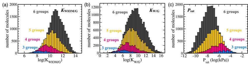
E. Lumiaro et al.: Predicting gas–particle partitioning coefficients of atmospheric molecules                               13229

rials science, machine learning is more established and now      Cumby, 2020; Himanen et al., 2020). We test several descrip-
frequently complements theoretical or experimental methods       tor choices here: the many-body tensor representation (Huo
(Müller et al., 2016; Ma et al., 2015; Shandiz and Gauvin,       and Rupp, 2017), the Coulomb matrix (Rupp et al., 2012), the
2016; Gómez-Bombarelli et al., 2016; Bartók et al., 2017;        Molecular ACCess System (MACCS) structural key (Durant
Rupp et al., 2018; Goldsmith et al., 2018; Meyer et al., 2018;   et al., 2002), a topological fingerprint developed by RDKit
Zunger, 2018; Gu et al., 2019; Schmidt et al., 2019; Coley et    (Landrum, 2006) based on the daylight fingerprint (James
al., 2020a; Coley et al., 2020b). Here we build on our experi-   et al., 1995), and the Morgan fingerprint (Morgan, 1965).
ence in atomistic, molecular machine learning (Ghosh et al.,        Our work addresses the following objectives: (1) with a
2019; Todorović et al., 2019; Stuke et al., 2019; Himanen       view to future machine learning applications in atmospheric
et al., 2020; Fang et al., 2021) to train a regression model     science, we assess the predictive capability of different struc-
that maps molecular structures onto saturation vapour pres-      tural descriptors for machine learning the chosen target prop-
sures and partitioning coefficients. Once trained, the machine   erties. (2) We quantify the predictive power of our machine
learning model can make saturation vapour pressure and par-      learning model for Wang’s dataset to ascertain if the dataset
titioning predictions at COSMOtherm accuracy for hundreds        size is sufficient for accurate machine learning predictions.
of thousands of new molecules at no further computational        (3) We then apply our validated machine learning model to
cost. When experimental training data become available, the      a new molecular dataset to gain chemical insight into SOA
machine learning model could easily be extended to encom-        condensation processes.
pass predictions for experimental pressures and coefficients.       The paper is organized as follows. We describe our ma-
    Due to the above-mentioned lack of comprehensive exper-      chine learning methodology in Sect. 2, then present the ma-
imental databases for saturation vapour pressures and gas–       chine learning results in Sect. 3. Section 4 demonstrates how
liquid partitioning coefficients of polyfunctional atmospher-    we employed the trained model for fast prediction of molec-
ically relevant molecules, our machine learning model is         ular properties. We discuss our findings and present a sum-
based on the computational data by Wang et al. (2017). They      mary in Sect. 5.
computed the partitioning coefficients and saturation vapour
pressures for 3414 atmospheric secondary oxidation prod-
ucts obtained from the Master Chemical Mechanism (Jenkin         2     Methods
et al., 1997; Saunders et al., 2003) using a combination of
quantum chemistry and statistical thermodynamics as im-          Our machine learning approach has six components as illus-
plemented in the COSMOtherm approach (Klamt and Eck-             trated in Fig. 1. We start off with the raw data, which we
ert, 2000). The parent VOCs for the MCM dataset include          present and analyse in Sect. 2.1. The raw data are then trans-
most of the atmospherically relevant small alkanes (methane,     formed into a suitable representation2 for machine learn-
ethane, propane, etc.), alcohols, aldehydes, alkenes, ketones,   ing (step 2). We introduce five different representations in
and aromatics, as well as chloro- and hydrochlorocarbons,        Sect. 2.2, which we test in our machine learning model (see
esters, ethers, and a few representative larger VOCs such as     Sect. 3). Next we choose our machine learning method. Here
three monoterpenes and one sesquiterpene. Some inorganics        we use kernel ridge regression (KRR), which is introduced in
are also included. For technical details on the COSMOtherm       Sect. 2.3. After the machine learning model is trained in step
calculations performed by Wang et al., we refer to the COS-      4, we analyse its learning success in step 5. The results of
MOtherm documentation (Klamt and Eckert, 2000; Klamt,            this process are shown in Sect. 3. In this step we also make
2011) and a recent study by Hyttinen et al. (2020) in which      adjustments to the representation and the parameters of the
the conventions, definitions, and notations used in COS-         model to improve the learning (see the arrow from “Checks”
MOtherm are connected to those more commonly employed            to “Features” in Fig. 1). Finally, we use the best machine
in atmospheric physical chemistry. We especially note that       learning model to make predictions as shown in Sect. 4.
the saturation vapour pressures computed by COSMOtherm
correspond to the subcooled liquid state and that the parti-     2.1    Dataset
tioning coefficients correspond to partitioning between two
                                                                 In this work we are interested in the equilibrium partitioning
flat bulk surfaces in contact with each other. Actual parti-
                                                                 coefficients of a molecule between a water-insoluble organic
tioning between e.g. aerosol particles and the gas phase will
                                                                 matter (WIOM) phase and its gas phase (KWIOM/G ) as well
depend on further thermodynamic and kinetic parameters,
                                                                 as between the gas phase and an infinitely diluted water so-
which are not included here.
                                                                 lution. These coefficients are defined as
    We transform the molecular structures in Wang’s dataset
into atomistic descriptors more suitable for machine learning                  CWIOM
than the atomic coordinates or the commonly used simplified      KWIOM/G =           ,                                         (1)
                                                                                CG
molecular-input line-entry system (SMILES) strings. Opti-
mal descriptor choices have been the subject of increased           2 We use the words “representation” and “features” interchange-
research in recent years (Langer et al., 2020; Rossi and         ably.

https://doi.org/10.5194/acp-21-13227-2021                                         Atmos. Chem. Phys., 21, 13227–13246, 2021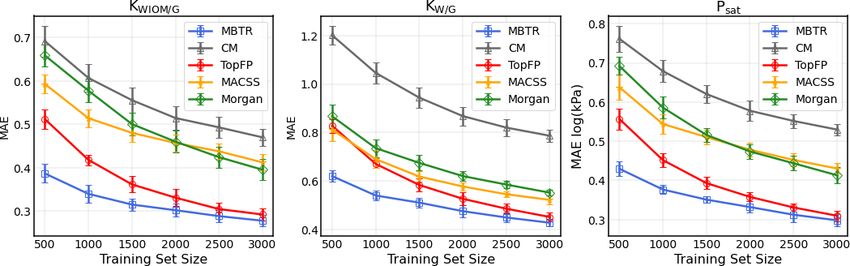
13230                          E. Lumiaro et al.: Predicting gas–particle partitioning coefficients of atmospheric molecules

Figure 1. Schematic of our machine learning workflow: the raw input data are converted into molecular representations (referred to as
features in this figure). We then set up and train a machine learning method. After evaluating its performance in step 5, we may adjust the
features. Once the machine learning model is calibrated and trained, we make predictions on new data.

Figure 2. Dataset statistics: panel (a) shows the size distribution (in terms of the number of non-hydrogen atoms) of all 3414 molecules
in the dataset. Panel (b) illustrates how many molecules contain each of the chemical species, and panel (c) depicts the functional group
distribution.

          CW
KW/G =       ,                                                 (2)      KW/G for 3414 molecules. These molecules were generated
          CG                                                            from 143 parent volatile organic compounds with the Master
where CWIOM , CW , and CG are the equilibrium concentra-                Chemical Mechanism (MCM) (Jenkin et al., 1997; Saunders
tions of the molecule in the WIOM, water, and gas phase, re-            et al., 2003) through photolysis and reactions with ozone, hy-
spectively, at the limit of infinite dilution. In the framework         droxide radicals, and nitrate radicals.
of COSMOtherm calculations, gas–liquid partitioning coef-                  Here, we analyse the composition of the publicly available
ficients can be converted into saturation vapour pressures, or          dataset by Wang et al. in preparation for machine learning.
vice versa, using the activity coefficients γW or γWIOM in the          Figure 2 illustrates key dataset statistics. Panel (a) shows the
corresponding liquid (which can also be computed by COS-                size distribution of molecules as measured in the number of
MOtherm). Specifically, if, for example, KW/G is expressed              non-hydrogen atoms. The 3414 non-radical species obtained
in units of m3 g−1 , then KW = MγRT          , where R is the gas       from the MCM range in size from 4 to 48 atoms, which trans-
                                      W Psat
constant, T the temperature, M the molar mass of the com-               lates into 2 to 24 non-hydrogen atoms per molecule. The
pound, and KW and γW the partitioning and activity coef-                distribution peaks at 10 non-hydrogen atoms and is skewed
ficients in water (Arp and Goss, 2009). This illustrates that           towards larger molecules. Panel (b) illustrates how many
unlike the saturation vapour pressure Psat , which is a pure            molecules contain at least one atom of the indicated element.
compound property, the partitioning coefficient also depends            All molecules contain carbon (100 % C); 3410 contain hy-
on the activity of the molecule in the chosen liquid solvent,           drogen (H; 99.88 %) and 3333 also oxygen (O; 97.63 %).
in this case water. We caution, however, that many different            Nitrogen (N) is the next most abundant element (30.17 %)
conventions exist e.g. for the dimensions of the partitioning           followed by chlorine (Cl; 3.05 %), sulfur (S; 0.44 %), and
coefficients and the reference states for activity coefficients         bromine (Br; 0.32 %). Lastly, panel (c) presents the distri-
– the relation given above applies only to the particular con-          bution of functional groups. It peaks at two (34 %) to three
ventions used by COSMOtherm. We refer to Hyttinen et al.                (31 %) functional groups per molecule, with relatively few
(2020) for a discussion on the connection between different             molecules having zero (2 %), five (3 %), or six (2 %) func-
conventions and the notation used by COSMOtherm, as well                tional groups. The percentages for one and four functional
as those commonly employed in atmospheric physical chem-                groups are 11 % and 17 %, respectively.
istry.                                                                     Figure 3 shows the distribution of the target properties
   Wang et al. (2017) used the conductor-like screening                 KWIOM/G , KW/G , and Psat in Wang’s dataset on a logarith-
model for real solvents (COSMO-RS) theory (Klamt and                    mic scale. The equilibrium partitioning coefficient KWIOM/G
Eckert, 2000; Klamt, 2011) implemented in COSMOtherm
to calculate the two partitioning coefficients KWIOM/G 3 and            tative secondary organic aerosol constituent. The IUPAC name
                                                                        for the compound in question, with elemental composition
   3 As a model WIOM phase Wang et al. used a compound                  C14 H16 O5 , is 1-(5-(3,5-dimethylphenyl)dihydro-[1,3]dioxolo[4,5-
originally suggested by Kalberer et al. (2004) as a represen-           d][1,3]dioxol-2-yl)ethan-1-one.

Atmos. Chem. Phys., 21, 13227–13246, 2021                                                https://doi.org/10.5194/acp-21-13227-2021
E. Lumiaro et al.: Predicting gas–particle partitioning coefficients of atmospheric molecules                                       13231

Figure 3. Dataset statistics: distributions of equilibrium partitioning coefficients (a) KWIOM/G , (b) KW/G , and (c) the saturation vapour
pressure Psat for all 3414 molecules in the dataset.

distribution is skewed slightly towards larger coefficients, in         2015; Huo and Rupp, 2017; Langer et al., 2020; Himanen
contrast to the saturation vapour pressure Psat distribution            et al., 2020).
that exhibits an asymmetry towards molecules with lower                    In this work we employ two classes of representations for
pressures. All three target properties cover approximately              the molecular structure, also known as descriptors: physi-
15 logarithmic units and are approximately Gaussian dis-                cal and cheminformatics descriptors. Physical descriptors en-
tributed. Such peaked distributions are often not ideal for             code physical distances and angles between atoms in the ma-
machine learning since they overrepresent molecules near the            terial or molecule. Meanwhile, decades of research in chem-
peak of the distribution and underrepresent molecules at their          informatics have produced topological descriptors that en-
edges. The data peak does supply enough similarity to ensure            code the qualitative aspects of molecules in a compact rep-
good-quality learning, but properties of the underrepresented           resentation. These descriptors are typically bit vectors, in
molecular types might be harder to learn.                               which molecular features are encoded (hashed) into binary
   We found 11 duplicate entries in Wang’s dataset. These               fingerprints, which are joined into long binary vectors. In
are documented in Sect. A in Table A1. The entries have                 this work, we use two physical descriptors, the Coulomb ma-
the same SMILES strings and chemical formula but differ in              trix and the many-body tensor, and three cheminformatics
their Master Chemical Mechanism ID. Also, the three target              descriptors: the MACCS structural key, the topological fin-
properties differ slightly. These duplicates did not affect the         gerprint, and the Morgan fingerprint.
learning quality, so we did not remove them from the dataset.              In Wang’s dataset the molecular structure is encoded
   Wang’s dataset of 3414 molecules is relatively small for             in SMILES (simplified molecular-input line-entry system)
machine learning, which often requires hundreds of thou-                strings. We convert these SMILES strings into structural de-
sands to millions of training samples (Pyzer-Knapp et al.,              scriptors using Open Babel (O’Boyle et al., 2011) and the
2015; Smith et al., 2017; Stuke et al., 2019; Ghosh et al.,             DScribe library (Himanen et al., 2020) or into cheminfor-
2019). A slightly larger set of Henry’s law constants, which            matics descriptors using RDKit (Landrum, 2006).
are related to KW/G , was reported by Sander (2015) for 4632
organic species. Sander’s database is a collection of 17 350            2.2.1   Coulomb matrix
Henry’s law constant values collected from 689 references
and therefore not as internally consistent as Wang’s dataset.           The Coulomb matrix (CM) descriptor is inspired by an elec-
For example, the Sander dataset contains several molecules              trostatic representation of a molecule (Rupp et al., 2012). It
with multiple entries for the same property, sometimes span-            encodes the Cartesian coordinates of a molecule in a simple
ning many orders of magnitude. We are not aware of a larger             matrix of the form
dataset that reports partitioning coefficients. For this reason,               (
we rely exclusively on Wang’s dataset and show that we can                       0.5Zi2.4 if i = j
                                                                        Cij =       Zi Zj                ,                        (3)
develop machine learning methods that are just as accurate as                     kR i −R j k if i 6 = j
the underlying calculations and thus suitable for predictions.
                                                                        where R i is the coordinate of atom i with atomic charge Zi .
                                                                        The diagonal provides element-specific information. The co-
2.2   Representations
                                                                        efficient and the exponent have been fitted to the total ener-
                                                                        gies of isolated atoms (Rupp et al., 2012). Off-diagonal el-
The molecular representation for machine learning should                ements encode inverse distances between the atoms of the
fulfil certain requirements. It should be invariant with re-            molecule by means of a Coulomb-repulsion-like term.
spect to translation and rotation of the molecule and permu-               The dimension of the Coulomb matrix is chosen to fit the
tations of atomic indices. Furthermore, it should be continu-           largest molecule in the dataset; i.e. it corresponds to the num-
ous, unique, compact, and efficient to compute (Faber et al.,           ber of atoms of the largest molecule. The “empty” rows of

https://doi.org/10.5194/acp-21-13227-2021                                              Atmos. Chem. Phys., 21, 13227–13246, 2021
13232 E. Lumiaro et al.: Predicting gas–particle partitioning coefficients of atmospheric molecules
Figure 4. Pictorial overview of descriptors used in this work: (a) ball-and-stick model of 2-hydroxy-2-methylpropanoic acid, (b) corre-
sponding Coulomb matrix (CM), (c) the O–H, O–O, and O–C inverse distance entries of the many-body tensor representation (MBTR), (d)
topological fingerprint (TopFP) depiction of a path with length 3, and (e) Morgan circular fingerprint with radius 0 (black), radius 1 (blue),
and radius 2 (orange).
Coulomb matrices for smaller molecules are padded with ze- 2.2.3 MACCS structural key
roes. Invariance with respect to the permutation of atoms in
the molecule is enforced by simultaneously sorting rows and The Molecular ACCess System (MACCS) structural key is a
columns of each Coulomb matrix in descending order ac- dictionary-based descriptor (Durant et al., 2002). It is repre-
cording to their `2 norms. An example of a Coulomb matrix sented as a bit vector of Boolean values that encode answers
for 2-hydroxy-2-methylpropanoic acid is shown in Fig. 4b. to a set of predefined questions. The MACCS structural key
The CM is easily understandable, simple, and relatively we used is a 166 bit long set of answers to 166 questions such
small as a descriptor. However, it performs best with Lapla- as “is there an S–S bond?” or “does it contain iodine?” (Lan-
cian kernels in the machine learning model (see Sect. 2.3), drum, 2006; James et al., 1995).
while other descriptors work better with the more standard MACCS is the smallest of the five descriptors and ex-
choice of a Gaussian kernel. tremely fast to use. Its accuracy critically depends on how
well the 166 questions encapsulate the chemical detail of the
2.2.2 Many-body tensor representation molecules. Is it likely to reach moderate accuracy with low
computational cost and memory usage, and it could be bene-
The many-body tensor representation (MBTR) follows the ficial for fast testing of a machine learning model.
Coulomb matrix philosophy of encoding the internal coordi-
nates of a molecule. We will describe the MBTR only quali- 2.2.4 Topological fingerprint
tatively here. Detailed equations can be found in the original
publication (Huo and Rupp, 2017), our previous work (Hi- The topological fingerprint (TopFP) is RDKit’s original fin-
manen et al., 2020; Stuke et al., 2020), and Appendix B. gerprint (Landrum, 2006) inspired by the Daylight finger-
Unlike the Coulomb matrix, the many-body tensor is con- print (James et al., 1995). TopFP first extracts all topologi-
tinuous and it distinguishes between different types of inter- cal paths of certain lengths. The paths start from one atom
nal coordinates. At many-body level 1, the MBTR records in a molecule and travel along bonds until k bond lengths
the presence of all atomic species in a molecule by plac- have been traversed as illustrated in Fig. 4d. The path de-
ing a Gaussian at the atomic number on an axis from 1 to picted in the figure would be OCCO. The list of patterns pro-
the number of elements in the periodic table. The weight of duced is exhaustive: every pattern in the molecule, up to the
the Gaussian is equal to the number of times the species is path length limit, is generated. Each pattern then serves as a
present in the molecule. At many-body level 2, inverse dis- seed to a pseudo-random number generator (it is “hashed”),
tances between every pair of atoms (bonded and non-bonded) the output of which is a set of bits (typically 4 or 5 bits per
are recorded in the same fashion. Many-body level 3 adds pattern). The set of bits is added (with a logical OR) to the
angular information between any triple of atoms. Higher lev- fingerprint. The length of the bit vector, maximum and min-
els (e.g. dihedral angles) would in principle be straightfor- imum possible path lengths kmax and kmin , and the length of
ward to add but are not implemented in the current MBTR one hash can be optimized.
versions (Huo and Rupp, 2017; Himanen et al., 2020). Fig- Topology is an informative molecular feature. We there-
ure 4c shows selected MBTR elements for 2-hydroxy-2- fore expect TopFP to balance good accuracy with reasonable
methylpropanoic acid. computational cost. However, this binary fingerprint is diffi-
The MBTR is a continuous descriptor, which is advanta- cult to visualize and analyse for chemical insight.
geous for machine learning. However, MBTR is by far the
largest descriptor of the five we tested, and this can pose re-
strictions on memory and computational cost. Furthermore,
the MBTR is more difficult to interpret than the CM.
Atmos. Chem. Phys., 21, 13227–13246, 2021 https://doi.org/10.5194/acp-21-13227-2021E. Lumiaro et al.: Predicting gas–particle partitioning coefficients of atmospheric molecules 13233
2.2.5 Morgan fingerprint The regression coefficients αi can be solved by minimiz-
ing the error:
The Morgan fingerprint is also a bit vector constructed by
hashing the molecular structure. In contrast to the topologi- n
X
cal fingerprint, the Morgan fingerprint is hashed along circu- min (f (x i ) − yi )2 + λα T Kα, (7)
α
lar or spherical paths around the central atom as illustrated i=1
in Fig. 4e. Each substructure for a hash is constructed by
where yi represents reference target values for molecules in
first numbering the atoms in a molecule with unique inte-
the training data. The second term is the regularization term,
gers by applying the Morgan algorithm. Each uniquely num-
whose size is controlled by the hyperparameter λ. K is the
bered atom then becomes a cluster centre, around which we
kernel matrix of training inputs k(x i , x j ).
iteratively increase a spherical radius to include the neigh-
This minimization problem can be solved analytically for
bouring bonded atoms (Rogers and Hahn, 2010). Each radius
the expansion coefficients αi .
increment extends the neighbour list by another molecular
bond. The “circular” substructures found by the algorithm α = (K − λI)−1 y (8)
described above, excluding duplicates, are then hashed into a
fingerprint (James et al., 1995; Landrum, 2006). The length The hyperparameters γ and λ need to be optimized sepa-
of the fingerprint and the maximum radius can be optimized. rately.
The Morgan fingerprint is quite similar to the TopFP in We implemented KRR in Python using scikit-learn (Pe-
size and type of information encoded, so we expect similar dregosa et al., 2011). Our implementation has been described
performance. It also does not lend itself to easy chemical in- in Stuke et al. (2019, 2020).
terpretation.
2.3.2 Computational execution
2.3 Machine learning method
Data used for supervised machine learning are typically di-
2.3.1 Kernel ridge regression
vided into two sets: a large training set and a small test set.
In this work, we apply the kernel ridge regression (KRR) Both sets consists of input vectors and corresponding target
machine learning method. KRR is an example of supervised properties. The KRR model is trained on the training set, and
learning, in which the machine learning model is trained on its performance is quantified on the test set. At the outset,
pairs of input (x) and target (f ) data. The trained model then we separate a test set of 414 molecules. From the remaining
predicts target values for previously unseen inputs. In this molecules, we choose six different training sets of size 500,
work, the input x represents the molecular descriptors CM 1000, 1500, 2000, 2500, and 3000 so that a smaller training
and MBTR as well as the MACCS, TopFP, and Morgan fin- size is always a subset of the larger one. Training the model
gerprints. The targets are scalar values for the equilibrium on a sequence of such training sets allows us to compute a
partitioning coefficients and saturation vapour pressures. learning curve, which facilitates the assessment of learning
KRR is based on ridge regression, in which a penalty for success with increasing training data size. We quantify the
overfitting is added to an ordinary least squares fit (Friedman accuracy of our KRR model by computing the mean abso-
et al., 2001). In KRR, unlike ridge regression, a nonlinear lute error (MAE) for the test set. To get statistically mean-
kernel is applied. This maps the molecular structure to our ingful results, we repeat the training procedure 10 times. In
target properties in a high-dimensional space (Stuke et al., each run, we shuffle the dataset before selecting the training
2019; Rupp, 2015). and test sets so that the KRR model is trained and tested on
The target values f are a linear expansion in kernel ele- different data each time. Each point on the learning curves
ments: is computed as the average over 10 results, and the spread
serves as the standard deviation of the data point.
n
X Model training proceeds by computing the KRR regres-
f (x) = αi k(x i , x), (4)
sion coefficients αi , obtained by minimizing Eq. (7). KRR
i=1
hyperparameters γ and λ are typically optimized via grid
where the sum runs over all training molecules. In this work, search, and average optimal solutions are obtained by cross-
we use two different kernels, the Gaussian kernel, validating the procedure. In cross-validation we split off a
0 2 validation set from the training data before training the KRR
kG (x, x 0 ) = e−γ kx−x k2 , (5) model. KRR is then trained for all possible combinations
of discretized hyperparameters (grid search) and evaluated
and the Laplacian kernel,
on the validation set. This is done several times so that
0
kL (x, x 0 ) = e−γ kx−x k1 . (6) the molecules in the validation set are changed each time.
Then the hyperparameter combination with minimum aver-
The kernel width γ is a hyperparameter of the KRR model. age cross-validation error is chosen. Our implementation of
https://doi.org/10.5194/acp-21-13227-2021 Atmos. Chem. Phys., 21, 13227–13246, 202113234 E. Lumiaro et al.: Predicting gas–particle partitioning coefficients of atmospheric molecules
a cross-validated grid search is also based on scikit-learn (Pe- Fig. 3, so this amounts to only 2.7 % of the entire range of
dregosa et al., 2011). The optimized values for γ and λ are values. Our best machine learning MAEs are of the order of
listed in Table B2. the COSMOtherm prediction accuracy, which lies at around a
Table 1 summarizes all the hyperparameters optimized in few tenths of log values (Stenzel et al., 2014; Schröder et al.,
this study, those for KRR and the molecular descriptors, and 2016; van der Spoel et al., 2019).
their optimal values. In the grid search, we varied both γ Figure 6 shows the results for the best-performing descrip-
and λ by 10 values between 10−1 and 1010 . In addition, we tors MBTR and TopFP in more detail. The scatter plots il-
used two different kernels, Laplacian and Gaussian. We com- lustrate how well the KRR predictions match the reference
pared the performance of the two kernels for the average of values. The match is further quantified by R 2 values. For
five runs for each training size, and the most optimal ker- all three target values, the predictions hug the diagonal quite
nel was chosen. In cases in which both kernels performed closely, and we observe only a few outliers that are further
equally well, e.g. for the fingerprints, we chose the Gaussian away from the diagonal. The predictions of the partitioning
kernel for its lower computational cost. coefficient KWIOM/G are most accurate. This is expected be-
To compute the MBTR and CM descriptors we employed cause the MAE in Table 2 is lowest for this property. The
the Open Babel software to convert the SMILES strings largest scatter is observed for partitioning coefficient KW/G ,
provided in the Wang et al. dataset into three-dimensional which has the highest MAE in Table 2.
molecular structures. We did not perform any conformer
search. MBTR hyperparameters and TopFP hyperparameters
were optimized by grid search for several training set sizes 4 Predictions
(MBTR for sizes 500, 1500, and 3000 and TopFP for sizes
1000 and 1500), and the average of two runs for each train- In the previous section we showed that our KRR model
ing size was taken. We did not extend the descriptor hyperpa- trained on the Wang et al. dataset produces low prediction
rameter search to larger training set sizes, since we found that errors for molecular partitioning coefficients and saturation
the hyperparameters were insensitive to the training set size. vapour pressures and can now be employed as a fast predic-
The MBTR weighting parameters were optimized in eighty tor. When shown further molecular structures, it can make in-
steps between 0 (no weighting) and 1.4 and the broadening stant predictions for the molecular properties of interest. We
parameters in six steps between 10−1 and 10−6 . The length demonstrate this application potential on an example dataset
of TopFP was varied between 1024 and 8192 (size can be var- generated to imitate organic molecules typically found in the
ied by 2n ). The range for the maximum path length extended atmosphere.
from 5 to 11, and the bits per hash were varied between 3 and Atmospheric oxidation reaction mechanisms can be gener-
16. ally classified into two main types: fragmentation and func-
tionalization (Kroll et al., 2009; Seinfeld and Pandis, 2016).
For SOA formation, functionalization is more relevant, as it
3 Results leads to products with intact carbon backbones and added
polar (and volatility-lowering) functional groups. Many of
In Fig. 5 we present the learning curves for our objectives the most interesting molecules from an SOA-forming point
KWIOM/G , KW/G , and Psat . Shown is the mean average er- of view, e.g. monoterpenes, have around 10 carbon atoms
ror (MAE) as a function of the training set size for all three (Zhang et al., 2018). These compounds simultaneously have
target properties and for all five molecular descriptors. As high enough emissions or concentrations to produce appre-
expected, the MAE decreases as the training size increases. ciable amounts of condensable products, while being large
For all target properties, the lowest errors are achieved with enough for those products to have low volatility.
MBTR, and the worst-performing descriptor is CM. TopFP We thus generated a dataset of molecules with a backbone
approaches the accuracy of MBTR as the training size in- of 10 carbon (C10) atoms. For simplicity, we used a linear
creases and appears likely to outperform MBTR beyond the alkane chain. In analogy to Wang’s dataset, we then deco-
largest training size of 3000 molecules. rated this backbone with zero to six functional groups at dif-
Table 2 summarizes the average MAEs and their standard ferent locations. We limited ourselves to the typical groups
deviations for the best-trained KRR model (training size of formed in “functionalizing” oxidation of VOCs by both of
3000 with MBTR descriptor). The highest accuracy is ob- the main daytime oxidants OH and O3 : carboxyl (-COOH),
tained for partitioning coefficient KWIOM/G , with a mean av- carbonyl (=O), and hydroxyl (-OH) (Seinfeld and Pandis,
erage error of 0.278, i.e. only 1.9 % of the entire KWIOM/G 2016). The (-COOH) group can only be added to the ends
range. The second-best accuracy is obtained for saturation of the C10 molecule, while (=O) and (-OH) can be added to
vapour pressure Psat with an MAE of 0.298 (or 2.0 % of the any carbon atom in the chain. We then generated all pos-
range of pressure values). The lowest accuracy is obtained sible arrangements combinatorially and filtered out dupli-
for KW/G with an MAE of 0.428. However, the range for cates resulting from symmetric combinations of functional
partitioning coefficient KW/G is also the largest, as seen in groups. In total we obtained 35 383 unique molecules. Ex-
Atmos. Chem. Phys., 21, 13227–13246, 2021 https://doi.org/10.5194/acp-21-13227-2021E. Lumiaro et al.: Predicting gas–particle partitioning coefficients of atmospheric molecules 13235
Table 1. All the hyperparameters that were optimized.
Hyperparameters Optimized values
KRR width of the kernel γ , regularization parameter λ descriptor-dependent
MBTR broadening parameters σ2 , σ3 ; weighting parameters w2 , w3 0.0075, 0.1; 1.2, 0.8
TopFP vector length; maximum path length kmax ; bits per hash 8192; 8; 16
Morgan vector length; radius 2048; 2
Figure 5. The learning curves for equilibrium partitioning coefficients KWIOM/G , KW/G , and saturation vapour pressure Psat for predictions
made with all five descriptors.
ample molecules are depicted in Fig. 9. While the functional are on average larger4 than those contained in Wang’s dataset
group composition of our C10 dataset is atmospherically rel- (Fig. 2). However, as seen from Fig. 8, the averages of all
evant, the particular molecules are not. The purpose of this three quantities (for a given number of functional groups)
dataset is to perform a relatively simple sanity check of the are not substantially different, illustrating the similarity of
machine learning predictions on a set of compounds struc- the two datasets. A certain degree of similarity is required
turally different from those in the training dataset. We note to ensure predictive power, since machine learning models
that using e.g. more atmospherically relevant compounds do not extrapolate well to data that lie outside the training
such as α-pinene oxidation products for this purpose might range.
be counterproductive, since Wang et al.’s dataset used for The variation in the studied parameters is larger in Wang’s
training contains several such compounds. dataset for molecules with four or fewer functional groups
For each of the 35 383 molecules, we generated a SMILES but similar or smaller for molecules with five or six func-
string that serves as input for the TopFP fingerprint. We did tional groups. This is likely the case because Wang’s dataset
not relax the geometry of the molecules with force fields or contains relatively few compounds with more than four func-
density functional theory. We chose TopFP as a descriptor tional groups. The variation in the studied parameters (for
because its accuracy is close to that of the best-performing each number of functional groups) predicted for the C10
MBTR KRR model, but it is significantly cheaper to evalu- dataset is in line with the individual group contributions pre-
ate. TopFP is also invariant to conformer choices, since the dicted based on fits to experimental data, for example by
fingerprint is the same for all conformers of a molecule. We the SIMPOL model (Pankow and Asher, 2008) for satura-
then predicted Psat , KWIOM/G , and KW/G with the TopFP– tion vapour pressures. According to SIMPOL, a carboxylic
KRR model. acid group decreases the saturation vapour pressure at room
Figures 7 and 8 show the predictions of our TopFP–KRR temperature by almost a factor of 4000, while a ketone group
model for the C10 dataset. For comparison with Wang’s reduces it by less than a factor of 9. Accordingly, if interac-
dataset, we broke the histograms and analysis down by tions between functional groups are ignored, a dicarboxylic
the number of functional groups. For a given number of acid, for example, should have a saturation vapour pressure
functional groups, the partitioning coefficients for our C10 more than 100 000 times lower than a diketone with the same
dataset are somewhat higher, and the saturation vapour carbon backbone. This is remarkably consistent with Fig. 8,
pressures correspondingly somewhat lower, than in Wang’s where the variation of saturation vapour pressures for com-
dataset. This follows from the fact that our C10 molecules
4 Our C10 molecules range in size from 10 to 18 non-hydrogen
atoms since the largest of our molecules contains two carboxylic
acid and four ketone and/or hydroxyl groups.
https://doi.org/10.5194/acp-21-13227-2021 Atmos. Chem. Phys., 21, 13227–13246, 202113236 E. Lumiaro et al.: Predicting gas–particle partitioning coefficients of atmospheric molecules
Table 2. The mean average errors (MAEs) and the standard deviations for all the descriptors and target properties (equilibrium partitioning
coefficients KWIOM/G , KW/G , and saturation vapour pressure Psat ) with the largest possible training size of 3000.
KWIOM/G KW/G Psat
Descriptor MAE 1 MAE 1 MAE log(kPa) 1 log(kPa)
CM 0.470 ±0.020 0.787 ±0.028 0.530 ±0.016
MBTR 0.278 ±0.013 0.427 ±0.015 0.298 ±0.016
MACCS 0.412 ±0.020 0.522 ±0.020 0.431 ±0.014
Morgan 0.396 ±0.026 0.552 ±0.014 0.413 ±0.022
TopFP 0.292 ±0.014 0.451 ±0.021 0.310 ±0.014
Figure 6. Scatter plots for predictions of the partitioning coefficients of a molecule between water-insoluble organic matter and the gas phase
KWIOM/G , water and the gas phase KW/G , and the saturation vapour pressure Psat for the test set of 414 molecules using MBTR (top) and
TopFP (bottom). The prediction with the lowest mean average error was chosen for each scatter plot.
pounds with two functional groups in our C10 dataset is turn is a subset of “all molecules”, the lengths of the bars in
slightly more than 5 orders of magnitude. a given bin reflect the percentages of molecules with 7 or 8
Figure 7 illustrates the fact that the saturation vapour pres- O atoms. We observe that below 10−10 kPa, almost all C10
sure Psat decreases with increasing number of functional molecules contain 7 or 8 O atoms, as there is little grey visi-
groups as expected, whereas KWIOM/G and KW/G increase. ble in that part of the histogram. In the context of atmospheric
This is consistent with Wang’s dataset as shown in Fig. 8, chemistry, the least-volatile fraction of our C10 dataset corre-
where we compare averages between the two datasets. The sponds to LVOCs (low-volatility organic compounds), which
magnitude of the decrease (increase) amounts to approxi- are capable of condensing onto small aerosol particles but
mately 1 or 2 orders of magnitude per functional group and not actually forming them. Our results are thus in qualitative
is, again, consistent with existing structure–activity relation- agreement with recent experimental results by Peräkylä et al.
ships based on experimental data (e.g. Pankow and Asher, (2020), who concluded that the highly oxidized C10 products
2008; Compernolle et al., 2011; Nannoolal et al., 2008). of α-pinene oxidation are mostly LVOCs. However, we note
The region of low Psat is most relevant for atmospheric that the compounds measured by Peräkylä et al. are likely to
SOA formation. However, we caution that COSMOtherm contain functional groups not included in our C10 dataset, as
predictions have not yet been properly validated against ex- well as structural features such as branching and rings.
periments for this pressure regime. As discussed above, we Figure 9a and c show the molecular structures of the
can hope for order-of-magnitude accuracy at best. Figure 9b lowest-volatility compounds and the highest-volatility com-
shows histograms of only molecules with 7 or 8 oxygen pounds with 7 or 8 O atoms, respectively. The six shown
atoms. These are compared to the full dataset. Since the “8 highest-volatility compounds inevitably contain at least one
O atom set” is a subset of the “7 or 8 O atoms” set, which in carboxylic acid group, as we have restricted the number of
Atmos. Chem. Phys., 21, 13227–13246, 2021 https://doi.org/10.5194/acp-21-13227-2021E. Lumiaro et al.: Predicting gas–particle partitioning coefficients of atmospheric molecules 13237 Figure 7. Histograms of C10 TopFP–KRR predictions for (a) KWIOM/G , (b) KW/G , and (c) Psat . The histograms are divided into different numbers of functional groups. Molecules with two or fewer functional groups have been omitted from these histograms because their total number is very low in the C10 dataset. Figure 8. Box plot comparing C10 (in blue) with Wang’s dataset (in red) for KWIOM/G , KW/G , and Psat for different numbers of functional groups. Shown are the minimum, maximum, median, and first and third quartile. functional groups to six or fewer, and only the acid groups to obtain identical descriptors for different molecule struc- contain two oxygen atoms. Comparing the two sets, we see tures, even for this relatively small pool of molecules. The that the lowest-volatility compounds contain more hydroxyl MACCS fingerprint in particular produced over 500 dupli- groups and fewer ketone groups, while the highest-volatility cates (about 15 % of the dataset) because its query list is not compounds with 7 or 8 oxygen atoms contain almost no sufficiently descriptive of this molecule class. Some dupli- hydroxyl groups. This is expected, since e.g. a hydroxyl cates were also observed for TopFP (< 1.5 %), whereas phys- group lowers the saturation vapour pressure by over a fac- ical descriptors were both entirely unique, as expected. The tor of 100 at 298 K, while the effect of a ketone group is, original dataset itself contained 11 identical molecular struc- as previously noted, less than a factor of 9 according to the tures labelled with different SMILES strings, as mentioned SIMPOL model (Pankow and Asher, 2008). However, even in Sect. 2.1. Machine learning model checks revealed that the the lowest-volatility compounds (Fig. 9a) contain a few ke- number of duplicates in this study was small enough to have tone groups such that the numbers of hydrogen-bond donor a negligible effect on predictions (apart from the MACCS and acceptor groups are roughly similar. This result demon- key models), so we did not purge them. strates that unlike the simplest group contribution models such as SIMPOL, which would invariably predict that the lowest-volatility compounds in our C10 dataset should be 5 Conclusions the tetrahydroxydicarboxylic acids, both the original COS- MOtherm predictions and the machine learning model based In this study, we set out to evaluate the potential of the on them are capable of accounting for hydrogen-bonding in- KRR machine learning method to map molecular structures teractions between functional groups. As we did not include to its atmospheric partitioning behaviour and establish which conformational information for our C10 molecules in the ma- molecular descriptor has the best predictive capability. chine learning predictions, this is most likely due to struc- KRR is a relatively simple kernel-based machine learn- tural similarities between the C10 compounds and hydrogen- ing technique that is straightforward to implement and fast to bonding molecules in the training dataset. train. Given model simplicity, the quality of learning depends Lastly, we consider the issue of non-unique descriptors. strongly on the information content of the molecular descrip- Although the cheminformatics descriptors are fast to com- tor. More specifically, it hinges on how well each format en- pute and use, a duplicate check revealed that it is possible capsulates the structural features relevant to the atmospheric https://doi.org/10.5194/acp-21-13227-2021 Atmos. Chem. Phys., 21, 13227–13246, 2021
13238                          E. Lumiaro et al.: Predicting gas–particle partitioning coefficients of atmospheric molecules

Figure 9. (a) Atomic structure of the six molecules with the lowest predicted saturation vapour pressure Psat . (b) Psat histograms for
molecules containing 7 or 8 O atoms (orange) or only 8 O atoms (green). For reference, the histogram of all molecules (grey) is also shown.
(c) Atomic structure of the six molecules with 7 and 8 O atoms and the highest saturation vapour pressure Psat .

behaviour. The exhaustive approach of the MBTR descriptor                  Our results show that KRR can be used to train a model
to documenting molecular features has led to very good pre-             to predict COSMOtherm saturation vapour pressures, with
dictive accuracy in machine learning of molecular properties            error margins smaller than those of the original COSMOth-
(Stuke et al., 2019; Langer et al., 2020; Rossi and Cumby,              erm predictions. In the future, we will extend our training
2020; Himanen et al., 2020), and this work is no exception.             set to especially encompass atmospheric autoxidation prod-
The lightweight CM descriptor does not perform nearly as                ucts (Bianchi et al., 2019), which are not included in exist-
well, but these two representations from physical sciences              ing saturation vapour pressure datasets and for which exist-
provide us with an upper and lower limit on predictive accu-            ing prediction methods are highly uncertain. We also intend
racy.                                                                   to extend the machine learning model to predict a larger set
   Descriptors from cheminformatics that were developed                 of parameters computed by COSMOtherm, such as vapor-
specifically for molecules have variable performance. Be-               ization enthalpies, internal energies of phase transfer, and
tween them, the topological fingerprint leads to the best               activity coefficients in representative phases. While COS-
learning quality that approaches MBTR accuracy in the limit             MOtherm predictions for complex molecules such as autox-
of larger training set sizes. This is a notable finding, not            idation products also have large uncertainties, a fast and ef-
least because the relatively small TopFP data structures in             ficient “COSMOtherm-level” KRR predictor would still be
comparison to MBTR reduce the computational time and                    immensely useful, for example, for assessing whether a given
memory required for machine learning. MBTR encoding re-                 compound is likely to have extremely low volatility or not.
quires knowledge of the three-dimensional molecular struc-              Experimental volatility data for such compounds are also
ture, which raises the issue of conformer search. It is unclear         gradually becoming available, either through indirect infer-
which molecular conformers are relevant for atmospheric                 ence methods such as Peräkylä et al. (2020) or, for exam-
condensation behaviour, and COSMOtherm calculations on                  ple, from thermal desorption measurements (Li et al., 2020).
different conformers can produce values that are orders of              These can then be used to constrain and anchor the model and
magnitude apart. TopFP requires only connectivity informa-              also ultimately yield quantitatively reliable volatility predic-
tion and can be built from SMILES strings, eliminating any              tions.
conformer considerations (albeit at the cost of possibly losing
some information on e.g. intramolecular hydrogen bonds).
All this makes TopFP the most promising descriptor for fu-
ture machine learning studies in atmospheric science that we
have identified in this work.

Atmos. Chem. Phys., 21, 13227–13246, 2021                                                https://doi.org/10.5194/acp-21-13227-2021
E. Lumiaro et al.: Predicting gas–particle partitioning coefficients of atmospheric molecules                                       13239

Appendix A: Dataset duplicates

Table A1. Duplicates found in Wang et al.’s dataset: listed are the index in the dataset, the ID in the Master Chemical Mechanism (MCM_ID),
the corresponding SMILES string, the chemical formula, and the three target properties (KWIOM/G , KW/G , and Psat ).

         No.    Index    MCM_ID               SMILES                              Formula       KWIOM/G       KW/G           Psat
         1         83    MACRNB               CC(C=O)(CON(=O)=O)O                 C4H7NO5             5.51      3.42    4.33E-02
                  716    MACROHNO3            CC(C=O)(CON(=O)=O)O                 C4H7NO5             5.59       3.5    3.44E-02
         2       1943    CHOMOHCO3H           CC(C=O)(C(=O)OO)O                   C4H6O5              5.93      5.32    2.26E-02
                   84    COHM2CO3H            CC(C=O)(C(=O)OO)O                   C4H6O5              5.89      4.83    2.55E-02
         3        439    IEB1OOH              CC(C=O)(C(CO)O)OO                   C5H10O5             7.22      8.02    1.64E-04
                 2624    C57OOH               CC(C=O)(C(CO)O)OO                   C5H10O5             7.24      7.47    1.90E-04
         4        730    MACRNBCO3H           CC(CON(=O)=O)(C(=O)O)O              C4H7NO6             8.06      6.85    2.86E-04
                 2469    MACRNBCO2H           CC(CON(=O)=O)(C(=O)O)O              C4H7NO6             8.12      6.93    2.34E-04
         5        817    TDICLETH             C(=CCl)Cl                           C2H2Cl2             2.54      0.41   4.15E+01
                 3141    CDICLETH             C(=CCl)Cl                           C2H2Cl2             2.54      0.41   4.15E+01
         6        819    CHOMOHPAN            CC(C=O)(C(=O)OON(=O)=O)O            C4H5NO7             5.49      2.31    1.43E-01
                 1221    COHM2PAN             CC(C=O)(C(=O)OON(=O)=O)O            C4H5NO7             5.37      2.08    1.99E-01
         7        900    THEX2ENE             CC=CCCC                             C6H12                2.4    −0.92    1.95E+01
                 3372    CHEX2ENE             CC=CCCC                             C6H12                2.4    −0.92    1.94E+01
         8       1443    CPENT2ENE            CC=CCC                              C5H10                1.9    −0.86    7.84E+01
                 3119    TPENT2ENE            CC=CCC                              C5H10               1.91    −0.85    7.71E+01
         9       1649    CBUT2ENE             CC=CC                               C4H8                 1.5    −0.84    2.56E+02
                 1665    TBUT2ENE             CC=CC                               C4H8                1.49    −0.84    2.58E+02
         10      2188    CO2N3CHO             CC(=O)C(C=O)ON(=O)=O                C4H5NO5             5.16      2.62    1.22E-01
                 3040    C4CONO3CO            CC(=O)C(C=O)ON(=O)=O                C4H5NO5             5.21      2.72    1.05E-01
         11      2127    C59OOH               CC(CO)(C(=O)CO)OO                   C5H10O5             7.59      7.86    6.75E-05
                 2636    IEC1OOH              CC(CO)(C(=O)CO)OO                   C5H10O5             7.53      7.76    8.09E-05

https://doi.org/10.5194/acp-21-13227-2021                                              Atmos. Chem. Phys., 21, 13227–13246, 2021
You can also read