Longevity of small-scale ('baby') plumes and their role in lithospheric break-up
←
→
Page content transcription
If your browser does not render page correctly, please read the page content below
Geophys. J. Int. (2021) 227, 439–471                                                                                    https://doi.org/10.1093/gji/ggab223
Advance Access publication 2021 June 09
GJI Geodynamics and tectonics

Longevity of small-scale (‘baby’) plumes and their role in lithospheric
break-up

Alexander Koptev ,1 Sierd Cloetingh                                   2
                                                                          and Todd A. Ehlers                1
1 Department    of Geosciences, University of Tübingen, Tübingen 72074, Germany. E-mail: alexander.koptev@ifg.uni-tuebingen.de
2 Tectonics   Research Group, Utrecht University, Utrecht 3584 CS, Netherlands

Accepted 2021 June 7. Received 2021 May 20; in original form 2021 February 3

                                                                                                                                                              Downloaded from https://academic.oup.com/gji/article/227/1/439/6295312 by guest on 11 September 2021
                                          SUMMARY
                                          Controversy between advocates of ‘active’ (plume-activated) versus ‘passive’ (driven by exter-
                                          nal tectonic stresses) modes of continental rifting and break-up has persisted for decades. To
                                          a large extent, inconsistencies between observations and models are rooted in the conceptual
                                          model of plumes as voluminous upwellings of hot material sourced from the deep mantle.
                                          Such large-scale plumes are expected to induce intensive magmatism and topographic uplift,
                                          thereby triggering rifting. In this case of an ‘active’ rifting-to-break-up system, emplacement
                                          of plume-related magmatism should precede the onset of rifting that is not observed in many
                                          rifted continental margins, thus providing a primary argument in favour of an antiplume origin
                                          for continental break-up and supercontinent fragmentation. However, mantle plumes are not
                                          restricted to whole-mantle (‘primary’) plumes emanating from the mantle-core boundary but
                                          also include ‘secondary’ plumes originating from the upper mantle transition zone or shal-
                                          lower. Over the last decades a number of such ‘secondary’ plumes with horizontal diameters
                                          of only ∼100–200 km (therefore, sometimes also called ‘baby’ plumes) have been imaged in
                                          the upper mantle below Europe and China. The longevity of such small-scale plumes and their
                                          impact on geodynamics of continental break-up have so far not been explored. We present
                                          results of a systematic parametrical analysis of relatively small thermal anomalies seeded at
                                          the base of the lithosphere. In particular, we explore the effects of variations in initial plume
                                          temperature (T = 1500–1700 ◦ C) and size (diameter of 80–116 km), characteristics of the over-
                                          lying lithosphere (e.g. ‘Cratonic’, ‘Variscan’, ‘Mesozoic’ and oceanic) and intraplate tectonic
                                          regimes (neutral or far-field extension of 2–10 mm yr–1 ). In tectonically neutral regimes, the
                                          expected decay time of a seismically detectable ‘baby’-plume varies from ∼20 to >200 Myr
                                          and is mainly controlled by its initial size and temperature, whereas the effect of variations
                                          in the thermotectonic age of the overlying lithosphere is modest. These small but enduring
                                          plumes are able to trigger localized rifting and subsequent continental break-up occurring from
                                          ∼10 to >300 Myr after the onset of far-field extension. Regardless of the thermomechanical
                                          structure of the lithosphere, relatively rapid (tens of Myr) break-up (observed in models with
                                          a hot plume and fast extension) favours partial melting of plume material. In contrast, in the
                                          case of a long-lasting (a few hundreds of Myr) pre-break-up phase (relatively cold plume, low
                                          extension rate), rifting is accompanied by modest decompressional melting of only ‘normal’
                                          sublithospheric mantle. On the basis of the models presented, we distinguish two additional
                                          modes of continental rifting and break-up: (1) ‘semi-active’ when syn-break-up magmatism
                                          is carrying geochemical signatures of the deep mantle with deformation localized above the
                                          plume head not anymore connected by its tail to the original source of hot material and (2)
                                          ‘semi-passive’ when the site of final lithospheric rupture is controlled by a thermal anomaly of
                                          plume origin but without invoking its syn-break-up melting. These intermediate mechanisms
                                          are applicable to several segments of the passive continental margins formed during Pangea
                                          fragmentation.
                                          Key words: Continental tectonics: extensional; Dynamics of lithosphere and mantle;
                                          Hotspots; Intra-plate processes; Large igneous provinces; Rheology: crust and lithosphere.


C The Author(s) 2021. Published by Oxford University Press on behalf of The Royal Astronomical Society. This is an Open Access

article distributed under the terms of the Creative Commons Attribution License (http://creativecommons.org/licenses/by/4.0/), which
permits unrestricted reuse, distribution, and reproduction in any medium, provided the original work is properly cited.
                                                                                                                                                       439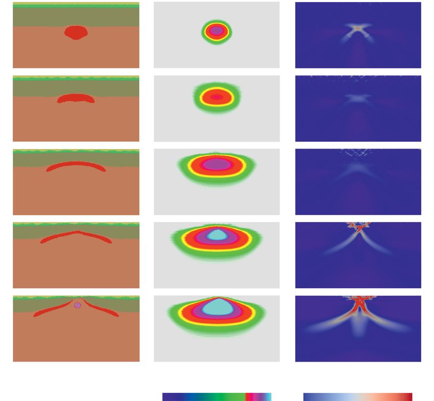
440      A. Koptev, S. Cloetingh and T.A. Ehlers

                                                                         mechanisms for the formation of several modern continental rifted
1 I N T RO D U C T I O N
                                                                         margins.
Most studies devoted to the interaction of the Earth’s lithosphere
with mantle hotspots are traditionally focused on classic Morgan-
type plumes originating from the lower mantle (Morgan 1971).
                                                                         2 B A C KG R O U N D
However, such ‘primary’ superplumes can stagnate beneath the
660 km phase change boundary and create numerous thermal pertur-         The origin of stresses in the lithosphere plays a key role in our
bations in the upper mantle corresponding to so-called ‘secondary’       understanding of geodynamic and geologic processes. Since the
plumes (Courtillot et al. 2003). According to predictions by Grif-       acceptance of continental drift (Holmes 1965) and plate tectonics
fiths & Campbell (1990) and Campbell & Griffiths (1990), mantle          (Wilson 1966) in the 1960s, three main sources have been recog-
upwelling from the core–mantle boundary should develop plume             nized for plate motions and stresses in the lithosphere, including:
heads of up to ∼2000 km in width after it flattens into a ‘pan-          (1) horizontal tractions at the base of the lithosphere arising from
cake’ shape beneath the lithosphere (Stern et al. 2020), whereas the     mantle convective flow (‘basal drag’), (2) forces exerted by cold,
heads of plumes originating within the upper mantle would have a         dense oceanic plates sinking into the mantle at a subduction zone
characteristic diameter of ∼600 km. Over the last decades a num-         due to its own weight (‘slab pull’) and (3) lateral variations in

                                                                                                                                                   Downloaded from https://academic.oup.com/gji/article/227/1/439/6295312 by guest on 11 September 2021
ber of much smaller plumes with horizontal size of only ∼100–            the lithosphere’s gravitational potential energy (topographic driv-
200 km (‘baby’ plumes) have been detected in the upper mantle            ing forces; e.g. ‘ridge push’). These mechanisms have been thor-
below Europe (Granet et al. 1995; Ritter et al. 2001; Babuška et al.    oughly explored by global (Forsyth & Uyeda 1975; Harper 1975;
2008) and China (Tang et al. 2014; Xia et al. 2016; Kuritani et al.      Richardson et al. 1979; Coblentz et al. 1994; Conrad & Lithgow-
2017).                                                                   Bertelloni 2002; Lithgow-Bertelloni & Guynn 2004; Bird et al.
   Despite the detected presence of these ‘baby’ plumes in various       2008; Koptev & Ershov 2010; Naliboff et al. 2012; Yang & Gurnis
areas around the globe (Ritter 2007; Xia et al. 2016) and their po-      2016) and regional (Wortel & Cloetingh 1985; Cloetingh & Wor-
tential importance for lithosphere break-up (Gac & Geoffroy 2009),       tel 1986; Richardson & Reding 1991; Coblentz & Sandiford 1994;
a systematic and comprehensive quantitative analysis of their prop-      Coblentz & Richardson 1996; Flesch et al. 2001; Liu & Bird 2002;
erties and impact on the overlying lithosphere has been lacking so       Reynolds et al. 2002; Burbidge 2004; Rajabi et al. 2017; Tunini
far. The bulk of previous numerical and analogue modelling stud-         et al. 2017) numerical modelling. Nevertheless, the driving mecha-
ies has explored consequences of plume-lithosphere interactions in       nism of plate tectonics still remains controversial. In particular, the
very different tectonic settings, including rifting/continental break-   role of upwelling mantle flow in the dynamics of continental rifting
up (Brune et al. 2013; Burov & Gerya 2014; Koptev et al. 2015,           and break-up systems (namely, ‘active’ versus ‘passive’ rifting) is
2016; Beniest et al. 2017a, 2017b), subduction initiation (Burov         a long-debated topic (e.g. Fitton 1983; Foulger et al. 2000; Foul-
& Cloetingh 2010; Gerya et al. 2015; Baes et al. 2020a, b, 2021;         ger & Hamilton 2014). In the ‘active’ or plume-assisted scenario
Cloetingh et al. 2021) and microcontinental separation (Dubinin          (Morgan 1971; Hill 1991), rifting occurs as a result of active mantle
et al. 2018; Koptev et al. 2019; Neuharth et al. 2021). However, all     diapirs rising through the mantle when extension is imparted by (1)
these studies have till now focused on relatively large (>>100 km in     horizontal viscous forces caused by radial flow of the plume head
the resulting horizontal size of the ‘pancake’-shaped head) mantle       below the lithosphere and (2) buoyancy forces associated with topo-
plume anomalies.                                                         graphic uplift over a plume (Westaway 1993). On the contrary, the
   Here we provide the first systematic analysis of small thermal        ‘passive’ scenario (McKenzie 1978) calls for the processes origi-
anomalies (‘baby’ plumes). In our experiments ‘baby’ plumes are          nating far away from the rifting zone when tensional far-field forces
initially seeded just below the bottom of the lithosphere. In this re-   (e.g. remote pull of the subducting slab) are transmitted through
spect, it is important to note that the source and emplacement mech-     the lithospheric plate causing its extension and thinning within a
anism of these small-scale thermal anomalies remains beyond the          localized area, while upwelling of underlying mantle and associ-
scope of our study. We intentionally focus on the consequences of        ated decompressional melting are both a passive consequence of
the implementation of the ‘baby’ plumes rather than on the scenarios     rifting-related stretching of the lithosphere.
for their origin, thus enabling a broad interpretation and applica-         This controversy between ‘active’ and ‘passive’ modes of rift-
tion of obtained modelling results. First, we explore the longevity      ing becomes even more critical when considering mechanisms of
of ‘baby’ plumes of different temperatures and sizes seeded un-          supercontinent break-up, a key component of the Earth’s tectonic
derneath different types of overlying lithosphere (i.e. lithospheres     and geodynamic evolution (Wilson 1966; Bradley 2011; Yoshida
of different thicknesses and different thermorheological structure).     & Santosh 2011). On the one hand, slab rollback is proven as a
Subsequently, we investigate the impact of ‘baby’ plumes on lo-          viable mechanism to induce extension in the overriding plate (e.g.
cation, timing and style (magmatic/amagmatic) of the break-up            Schellart & Moresi 2013; Holt et al. 2015; Yoshida 2017), whereby
when the overlying lithosphere is subjected to external tectonic ex-     the dragging force from slab retreat in oceanic subduction zones
tension. In our study, we pay particular attention to the temporal       surrounding a supercontinent (Collins 2003; Zhong et al. 2007)
evolution of the width of the thermal anomaly that permits us to test    has been proposed as the main driving mechanism for its dispersal
seismic detectability of the ‘baby’ plumes over the modelled time        (Bercovici & Long 2014). On the other hand, extension caused by
period.                                                                  subduction retreat has been shown to be focused along the marginal
   Our results are not only relevant for small plume anomalies           zones only while having far less impact on the interior of the su-
presently detected in Europe and China, but also important for pos-      percontinent (Zhang et al. 2018). According to this (Zhang et al.
sible scenarios for Pangea fragmentation complementing existing          2018) and other recent numerical models of global mantle convec-
end-member views on ‘active’ and ‘passive’ rifting and break-up.         tion (Huang et al. 2019; Dang et al. 2020), the main reason for
In particular, we resolve apparent contradictions and disputes on        supercontinent break-up resides in the push by the rise of mantle
non-plume and plume-driven break-up by introducing intermedi-            plumes from the subcontinental mantle (Li et al. 1999, 2008). Thick
ate (‘semi-active’ and ‘semi-passive’) modes which could be viable       mid-Jurassic oceanic crust in the Atlantic and Indian oceans is also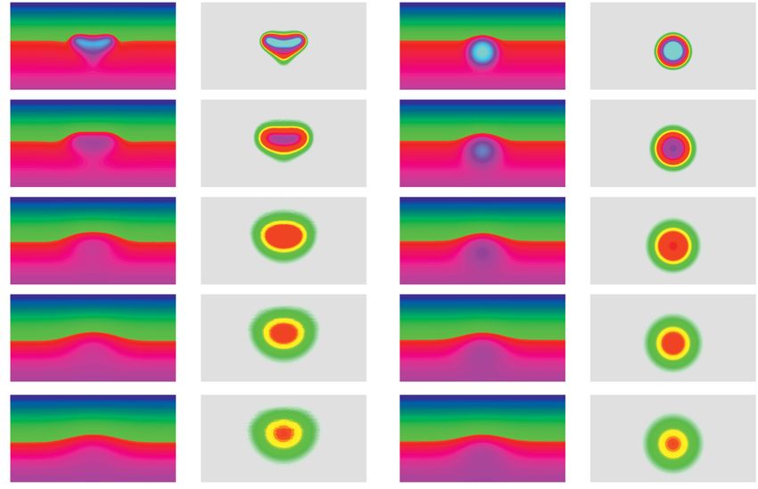
‘Baby’ plumes and break-up           441

indicative of hotter upper mantle underneath Pangea before the dis-      Romanowicz 2015; Davaille & Romanowicz 2020). In the prox-
integration of this supercontinent (Lenardic 2017; Van Avendonk          imity of these plumes mid-ocean ridges exhibit a greater overall
et al. 2017). As a step to reconcile these end-member views on the       content of volatiles and excess bathymetry (Gibson & Richards
dominant force responsible for supercontinent dispersal it has been      2018). Moreover, the geochemistry of LIPs has demonstrated a
demonstrated that deeply subducting slabs might penetrate into the       major contribution of undepleted material derived from primitive,
lower mantle and trigger upwelling and return flow that results in       undegassed reservoirs located in the lowermost mantle (Jackson
mantle superplumes (Zhang et al. 2010; Heron et al. 2015; Dal Zilio      et al. 2010, 2017). Finally, the fact that LIPs occur close to fi-
et al. 2018).                                                            nal break-up (Buiter & Torsvik 2014), and are frequently preceded
   The timing and volume of rift-related magmatism are tradition-        by long-lasting amagmatic phases of ‘passive’ rifting (Ziegler &
ally considered as a primary proxy for identification of the ‘ac-        Cloetingh 2004), cannot disprove a plume-triggered scenario when
tive’ component associated with mantle plume upwelling (Şengör         a mantle plume is emplaced below a lithosphere already extended
& Burke 1978). As has been noted for almost five decades (Scrut-         over a wide area (Reemst & Cloetingh 2000) localizing distributed
ton 1973), continental break-up in different parts of the Pangea         deformation in a narrow zone of break-up. By means of ultra-high
supercontinent was shortly preceded by intensive and massive mag-        resolution 3-D thermomechanical modelling, it has been shown that
matic events leading to the formation of so-called Large Igneous         in the case of a combined ‘active-passive’ scenario initial impinge-

                                                                                                                                                 Downloaded from https://academic.oup.com/gji/article/227/1/439/6295312 by guest on 11 September 2021
Provinces (LIPs). LIPs are large volumes of predominantly mafic          ment of a mantle plume can precede final break-up of the overlying
rocks that distinguish themselves from magma generated by pro-           lithosphere by up to 100 Myr under the condition of ultra-slow (half-
cesses at plate boundaries (Coffin & Eldholm 1994; Bryan & Ernst         rate of 2
offshore topographic uplift (Rohrman et al. 1995; Rohrman & van          Ga) Earth history (Dziewonski et al. 2010; Burke 2011; Torsvik
der Beek 1996; Japsen & Chalmers 2000; Koptev et al. 2017) along         et al. 2016).
the adjacent North Atlantic passive margins. The aforementioned             However, apart from this ‘Burke Earth’ end-member model
contradictions to an idealized plume-impingement model inspire a         (Torsvik et al. 2016) which is focused on first-order (or ‘primary’)
fundamental reappraisal of the causes for (super)continental break-      hotspots originating from the deep mantle (Fig. 1a1), other types
up and, in particular, their link to LIPs (Peace et al. 2020). This      of plumes have been proposed (Courtillot et al. 2003). In particu-
has fueled ‘antiplume’ conceptions and brought several authors to        lar, a ‘primary’ superplume stagnated at the base of, or within, the
argue in favour of shallow tectonics (i.e. ‘passive’) mechanisms         upper-lower mantle transition zone (MTZ: 410–660 km; Helffrich &
during break-up of different Pangea segments including those as-         Wood 2001) can create numerous thermal perturbations extending
sociated with LIPs and traditionally attributed to ‘active’ rifting      throughout the upper mantle, forming so-called ‘secondary’ plumes
mechanisms: break-up in North, Central and South Atlantic and in         which can further generate or contribute to the shallow ‘tertiary’
East and West Gondwana (Lundin & Doré 2005; Peace et al. 2020,          hotspots (Fig. 1a2). In contrast to the ‘primary’ and ‘secondary’
and references herein).                                                  plumes continuously fed from below (whether from LLSVPs at the
   However, all these ‘antiplume’/‘shallow tectonics’ scenarios and      core–mantle boundary or from bunched plume material at 660 km
views are in general at odds with findings from modern seismic to-       depth), ‘tertiary’ hotspots are traditionally thought to have an ex-
mography showing evidence for the widespread presence of low             clusively superficial origin being linked to tensile stresses and
velocity anomalies extending down to the core–mantle bound-              cracking in the lithosphere and decompressional melting (Courtillot
ary (Romanowicz & Gung 2002; Montelli et al. 2006; French &              et al. 2003; Torsvik et al. 2016). In another end-member scenario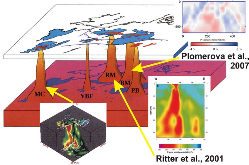
442 A. Koptev, S. Cloetingh and T.A. Ehlers
(a)
(b) (c) (d)
Downloaded from https://academic.oup.com/gji/article/227/1/439/6295312 by guest on 11 September 2021
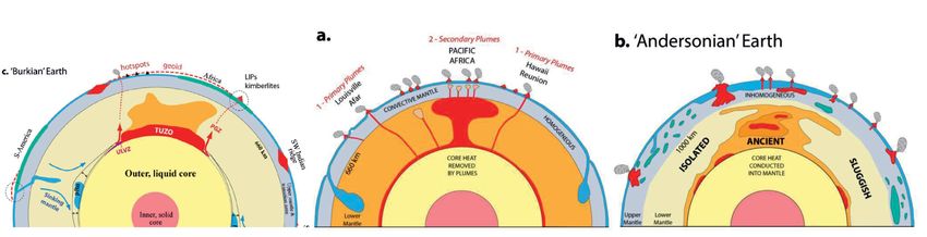
Figure 1. (a) Different models of internal Earth structure (from Torsvik et al. 2016): (a1) ‘Burke Earth’ with only ‘primary’ plumes derived from margins
of thermochemical piles (LLSVPs) at core–mantle boundary (Burke 2011); (a2) ‘Courtillot Earth’ with three types of ‘primary’, ‘secondary’ and ‘tertiary’
plumes (Courtillot et al. 2003); and (a3) ‘Andersonian Earth’ with only superficial ‘tertiary’ hotspots (Anderson 2000). Abbreviations: pBn, post-Bridgmentite;
PGZ, plume generation zone; ULVZ, ultra-low velocity zone. (b) Upwelling of small-scale mantle plumes (‘baby’ plumes) below European lithosphere (from
Granet et al. 1995). Insets are images from seismic tomography for French Massif Central (from Granet et al. 1995), Rhenish Massif/Eifel volcanic area
(from Ritter et al. 2001) and Bohemian Massif/Eger rift (from Plomerova et al. 2007). Abbreviations: MC, Massif Central; VBF, Vosges-Black Forest; RM,
Rhenish Massif; BM, Bohemian Massif; PB, Pannonian Basin. Areas in blue and red are Variscan basement massifs and Tertiary–Quaternary volcanic fields,
respectively. (c) Scenario illustrating hotspot organization in the Earth’s mantle beneath southernmost China (from Xia et al. 2016); (d) Structure and models
of volcanic passive margins: (d1) schematic cross-section along a volcanic passive margin: tectonic and magmatic segmentation controlled by asthenospheric
diapirs (from Geoffroy 2001). Abbreviations: M.C., magma chamber; SDV, seaward-dipping volcanic formations; (d2) initial geometry (left-hand panel) and
results (right-hand panel) of numerical modelling of the strain distribution in the lithosphere containing six aligned soft points corresponding to thermal
instabilities related to small-scale mantle diapirs (from Gac & Geoffroy 2009).
corresponding to the so-called ‘Andersonian Earth’ (Anderson 2006; Campbell 2007). Note that a symmetrical configuration might
2000) where any communication between the upper and lower man- be complicated by preexisting zones of lithospheric thinning acting
tle is excluded, these ‘tertiary’ hotspots become the only source of as sinks for a buoyant mantle plume (Sleep 1996, 1997). The result-
intraplate magmatism (Fig. 1a3). ing long-distance (>1000 km) propagation of hot plume material
Numerous examples can be given for each category of mantle up- along the elevated lithosphere–asthenosphere boundary is reflected
welling and associated thermal perturbations in the mantle (Cour- in alkaline volcanism (Ebinger & Sleep 1998) and regional uplift
tillot et al. 2003). Interaction of ‘primary’ plumes with oceanic (Koptev et al. 2017) in the areas remote from the point of initial
lithosphere is known to generate hotspot tracks characterized by the plume impingement. Given this strong filter of mantle plume activity
time progression of magmatism as a result of tectonic plates motion by thick continental lithosphere, evidence for hotspot chains within
over large-scale columnar upwelling in the mantle (Wilson 1963; continents is seldom. The commonly cited example of the Yellow-
Morgan 1972; Steinberger et al. 2004; Doubrovine et al. 2012; stone hotspot (Smith et al. 2009) demonstrates a time-progressive
Torsvik et al. 2017). Within continents, the sudden onset of conti- track in a direction that is not consistent with North American
nental flood volcanism over a large area of up to 106 km2 attributed plate motion (Jordan et al. 2004; Meigs et al. 2009; Wagner et al.
to melting of hot material from plume sources (Campbell & Griffiths 2010). The first confirmed example of a continental hotspot track
1990) is usually manifested in tens of Myr after initial plume-related aligned with plate motion has been recently detected in the eastern
surface uplift (Rainbird & Ernst 2001) of ∼0.5–2 km (Griffiths et al. United States, where a linear (∼200–250 km wide) seismic anomaly
1989; Farnetani & Richards 1994; Şengör 2001). This rapid, tran- with reduced P-wave velocity in the lower lithosphere (Chu et al.
sient domal uplift above the plume axis is followed by subsidence 2013) has been formed as a result of the westward passage of the
(Burov & Cloetingh 2009; Friedrich et al. 2018; Göğüş 2020) due to North American Plate (Cox & Arsdale 2002) over a ‘primary’,
flattening of the plume head below the base of the lithosphere (White deep-sourced thermal mantle plume presently located beneath the
& McKenzie 1989). The radial flow away from a plume’s axis leads Bermuda-Sargasso Sea region (Li et al. 2020). Based on combined
to a mushroom-like shape of the plume: a large disk-shaped head analysis of seismic tomography, uplift, volcanism and heat-flow
(∼1000 km in diameter) with a narrow long tail (Campbell & Davies data, three trajectories of separate hotspots have been also detected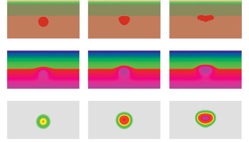
‘Baby’ plumes and break-up            443

below Arabia and the Horn of Africa (Vicente de Gouveia et al.           There, the ascent of the mantle plumes has been presumably caused
2018). In this case, however, these tracks correspond to distinct        by decompressional melting of nearly water-saturated material (so-
‘secondary’ plumes (Afar, East-Africa and Lake-Victoria) origi-          called ‘hydrous plumes’; Kuritani et al. 2017, 2019) in the MTZ
nated from the same deep-sourced (super)plume which raised from          (Fei et al. 2017; Fomin & Schiffer 2019; Long et al. 2019) where
LLSVPs but subsequently stagnated below the upper mantle tran-           an excess of fluids is commonly attributed to subduction of oceanic
sition zone at 660 km (Vicente de Gouveia et al. 2018). Similar          fluid-rich plates and their subsequent accumulation at the 660 km
‘secondary’ structures have been detected in the upper mantle be-        discontinuity boundary (Hetényi et al. 2009; Kovács et al. 2020).
neath Europe by seismologists during the last decades (Granet et al.     Alternatively, widespread intraplate volcanism in northeast China
1995; Ritter et al. 2000, 2001; Plomerova et al. 2007; Babuška et al.   above a stagnated Pacific slab has been explained by a return flow
2008; Fig. 1b). Given that they are characterized by extremely small     of sublithospheric mantle material entrained beneath the subduct-
horizontal sizes of ∼100 km, these structures have been dubbed           ing plate and then escaped through a gap in the slab resulting in
‘baby’ plumes (Cloetingh & Ziegler 2009). Apart from their small         focused ‘baby’-plume-like upwelling in the upper mantle (Tang
size, the ‘baby’ plumes also have a relatively small seismic velocity    et al. 2014). It is important to note that European ‘baby’ plumes are
contrast (< 3 per cent) with respect to the surrounding mantle and,      developed in conjunction with the Cenozoic rift system (Bourgeois
therefore, their detection requires specifically designed seismolog-     et al. 2007) formed within a continental foreland on the subducting

                                                                                                                                                  Downloaded from https://academic.oup.com/gji/article/227/1/439/6295312 by guest on 11 September 2021
ical experiments on a regional and local scale (Ritter 2005). The        plate (Ziegler & Dèzes 2007). This indicates, therefore, that em-
origin of these small-scale thermal anomalies characterized by a         placement of small-scale mantle anomalies might occur in a broad
modest excess of potential temperature of ∼150–200 ◦ C remains           spectrum of possible geodynamic settings across the subduction
controversial. Based on a global tomographic model, a deep magma         zone from foreland (Europe) to hinterland (China).
source in the lower mantle has been proposed (Goes et al. 1999,             Another observation that is known since almost two decades, but
2000). In contrast, the regional studies in the French Massif Central    so far not taken into consideration in the ‘baby’ plumes context, is
(Granet et al. 1995, Sobolev et al. 1997) and the Eifel volcanic         that volcanic passive margins are frequently punctuated every 50–
fields of northwestern Germany (Ritter et al. 2000, 2001) provide        150 km by long-lived igneous centers (Geoffroy 2001; Fig. 1d1).
evidence for the tail of a mantle plume extending only to a depth of     These are related to large crustal magma chambers developed over
300–400 km, thus indicating their shallower origin from the MTZ.         mantle diapirs which have been interpreted as a consequence of
It should be noted, however, that the plume tails in the MTZ and         small-scale convection cells at the level of the shallowest astheno-
deeper may not be visible in seismic tomography data because of          sphere (Geoffroy 2005). In view of their small (∼100 km) char-
their narrow width. The likely presence of plume conduits is indi-       acteristic size and moderate (∼150–200 K) temperature contrast it
rectly confirmed by volcanic rocks and gases in these regions which      seem to be reasonable to consider the mantle diapirs described by
often have the geochemical signatures of a deep source in the lower      Geoffroy (2001) as the equivalent of the ‘baby’ plumes discussed
mantle (Hoernle et al. 1995; Buikin et al. 2005; Caracausi et al.        above. It is also noteworthy that despite the relatively shallow depth
2016), although the interpretation of data is ambiguous (Lustrino &      extent of these mantle diapirs, the question on the origin of such
Carminati 2007). For the western Bohemian Massif, a low-velocity         ‘baby’ plumes of ‘tertiary’ class remains open and a potential role
anomaly beneath the Tertiary Eger Rift system is confined to a           of a deep mantle source in their establishment is feasible.
depth of 250 km (Plomerová et al. 2007, 2016; Babuška et al. 2008;        Despite their modest dimension and magnitude and regardless
Koulakov et al. 2009). This anomaly and associated magmatism (Ul-        of the mechanism of their emplacement, thermal instabilities re-
rych et al. 2011), therefore, could be attributed to the category of     lated to ‘baby’ plumes are known to have a pronounced expres-
‘tertiary’ hotspots which are presumably related to shallow tectonic     sion not only in magmatism (Wilson & Downes 1992) and verti-
processes and upwelling of the lithosphere–asthenosphere bound-          cal surface motions (Guillou-Frottier et al. 2007; Fauquette et al.
ary. However, a possible link to deeper sources (and thus belonging      2020; Kreemer et al. 2020) but also in the rheological structure of
to the category of ‘secondary’ plumes) is not to be excluded: the        the overlying lithosphere (Garcia-Castellanos et al. 2000; Tesauro
isolated bodies of thermal anomalies presently residing at shallow       et al. 2009a, b). This appears to be also the case for asthenospheric
depths might only have lost their initial connection with the deep       diapiric instabilities emplaced in volcanic rifted margin settings
source of hot material either due to exhaustion of this source or just   (Geoffroy 2001). There, the thermal consequences of mantle di-
because of plate movement. In the latter case, the head of such ‘sec-    apirs (or ‘baby’ plumes as we call them here) lead to the devel-
ondary’ plume has been attached to the bottom of the lithosphere         opment of the rheological soft-points which expectedly concen-
and subjected to lateral shift with respect to the feeding channel in    trate the regional extension around them. As shown by analogue
the sublithospheric mantle (i.e. plume tail).                            (Callot et al. 2002) and numerical (Gac & Geoffroy 2009) mod-
   More recently, seismological evidence for ‘baby’-plume-like           elling, initially isolated mantle soft points produce not only simul-
structures has been also obtained in the Western Pacific and ad-         taneous localized extension over them but also, given their narrow
jacent areas of mainland China (Tang et al. 2014; Xia et al. 2016;       spacing, interconnect zones of localized stretching ultimately lead-
Kuritani et al. 2017). In particular, a ‘primary’ plume with an ex-      ing to continental break-up and volcanic passive margin formation
tending columnar tail beneath southernmost China (Hainan Island          (Fig. 1d2).
area) appears to spread laterally within the MTZ, thus ponding at           Below two fundamental aspects are central. The first principal
the level of the lower part of the upper mantle. This ‘plume head’       question concerns the preservation in time of the plumes of differ-
is seated deeper than ‘normal’ ‘primary’ plumes (which are usually       ent scales after their emplacement. Because of long-term stability
flattened below the lithospheric bottom), and is further decomposed      of LLSVPs (from 200 Myr to >2 Gyr; see Burke 2011; Torsvik
into smaller separate patches (Xia et al. 2016), identical to ‘sec-      et al. 2016), ‘primary’ large-scale plumes can be preserved and re-
ondary’ ‘baby’ plumes proposed by Granet et al. (1995) for the           main seismologically detectable during hundreds of Myr. ‘Primary’
European region (compare Figs 1b and c). Similar finger-like upper       plumes of intermediate size potentially resulting in ‘hidden’ hotspot
mantle structures have been also detected below northeast China          tracks (as, for example, detected in the eastern USA by a few hun-
near the border between China and North Korea (Tang et al. 2014).        dred km wide corridor of low seismic velocities in the lithospheric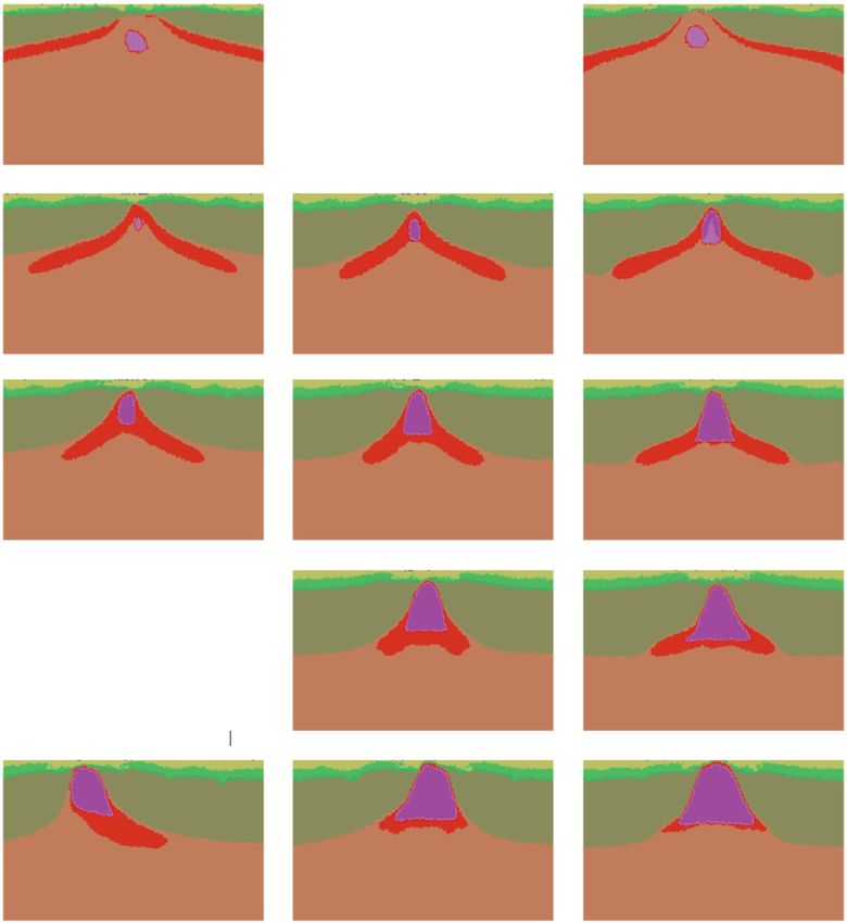
444 A. Koptev, S. Cloetingh and T.A. Ehlers
[μW × m−3 ]
Mantle density and heat capacity are computed as function of pressure and temperature using the Perple X algorithm (Connolly 2005) with the thermodynamic database taken from Holland & Powell (1998,
revised 2002) and the LOSIMAG composition by Hart & Zindler (1986). For the crustal rocks, heat capacity c p = 1000 J × kg−1 K−1 , whereas density is calculated from Boussinesq approximation:
ρ = ρ0 [1 − α(T − T0 )][1 + β(P − P0 )], where α = 3 × 10⁻⁵ K−1 is thermal expansion coefficient, β = 1 × 10⁻⁵ MPa−1 is adiabatic compressibility, and ρ0 is reference density (at P0 = 0.1 MPa and T0 =
mantle, see Chu et al. 2013) can survive more than 100 Myr accord-
0.022
0.024
ing to thermochemical numerical models by Yang & Leng (2014).
2.00
1.00
0.25
Hr
In contrast, small-scale mantle anomalies of ‘secondary’/‘tertiary’
Thermal parameters
category are known to produce no hotspot tracks associated with
the volcanism (e.g. Ritter et al. 2000, 2001) and the life span of
[W × m−1 × K−1 ]
these ‘baby’ plumes is still an open question. Although seismo-
T +77
T +77
T +77
T +77
T +77
1293
1293
807
807
474
298 K) which is taken as 2700 and 3000 kg × m−3 for upper and lower crust, respectively. Basaltic oceanic crust is modelled with the same material properties as mafic lower continental crust.
logical evidence apparently underpins their existence, it remains
unclear whether these tomographic snapshots are related to very re-
k
0.64 +
0.64 +
1.18 +
0.73 +
0.73 +
cent emplacement or whether these ‘baby’ plumes have a life span
long enough to still allow their detection for tens of million years or
even longer after impingement. The second key question concerns
the consequences of the small and isolated thermal anomalies for
0.25
0.25
0.25
0.25
0.25
ε1
break-up tectonics (Gac & Geoffroy 2009). Important is in this con-
text also their potential link to large-scale tectonic processes related
ε
to supercontinental fragmentation.
0.0
0.0
0.0
0.0
0.0
ε0
Downloaded from https://academic.oup.com/gji/article/227/1/439/6295312 by guest on 11 September 2021
3 METHODS
0.3
0.3
0.3
0.3
0.0
b1
Brittle
sin(ϕ)
3.1 Code description
0.6
0.6
0.6
0.6
0.1
b0
The numerical experiments presented here were conducted with a
2-D version of the thermomechanical viscous-plastic code I3ELVIS
(Gerya & Yuen 2007; Gerya 2010) that solves Stokes flow and heat
C1
3
3
3
3
3
C [MPa]
conservation equations using finite-differences combined with a
marker-in-cell technique. In this numerical scheme, physical prop-
C0
10
10
10
10
3
erties are transported by Lagrangian markers that move according
to the velocity field interpolated from the fixed fully staggered Eu-
lerian grid.
2.3
2.3
3.2
3.5
4.0
[J × MPa−1 × mol−1 ] n
The Stokes flow approximation is given by conservation of mo-
Rheological parameters
mentum:
∇ · η∇ν = ∇ P − ρg, (1)
and conservation of mass which is ensured by the incompressible
1.6
1.6
V
0
0
0
continuity equation:
∇ · ν = 0, (2)
Ductile
where η is the material viscosity, ν is the velocity field, P is the pres-
[kJ × mol−1 ]
sure, ρ is the density and g is the gravity acceleration (9.8 m × s−2 ).
154
154
238
532
470
E
The mechanical equations are coupled to the heat conservation
equation that takes the following form:
∂T
ρc p = ∇ · k∇T + ρ Hr , (3)
∂t
1.97 × 10¹⁷
1.97 × 10¹⁷
4.80 × 10²²
3.98 × 10¹⁶
5.01 × 10²⁰
[Pan × s]
AD
where T is the temperature, c p is the heat capacity, k is the thermal
conductivity and Hr is the radiogenic heat production (Table 1).
The code uses non-Newtonian viscoplastic rheologies (Burov
2011) where the viscosity for dislocation creep (ηcr eep ) is defined
Plagioclase (An75)
as follow (Karato & Wu 1993; Ranalli 1995; Ershov & Stephenson
Wet quartzite
Wet quartzite
Table 1. Rheological and thermal parameters.
Dry olivine
Wet olivine
Flow law
2006):
n1
1 E + PV 1−n
ηcreep = 2 A D exp ε̇II n , (4)
RT
where ε̇II = 1/2ε̇i j ε̇i j is the second invariant of the strain rate
tensor and A D , E, V , n and R are the pre-exponential constant, the
sublithospheric mantle
activation energy, the activation volume, the stress exponent, and
Felsic
Mafic
the gas constant (8.314 J × K−1 × mol−1 ), respectively (see also
Table 1). Different ductile flow law mechanisms such as diffusion
Mantle plume
Lithospheric/
Lower Crust
(Karato 1986), grain boundary sliding (Précigout et al. 2007) and
Upper crust
Peierls (Karato 2008) creep are neglected.
Material
In order to combine the ductile rheology with a brittle rheology,
the Mohr–Coulomb yield criterion (Ranalli 1995) is implemented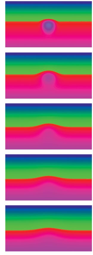
‘Baby’ plumes and break-up              445

by limiting creep viscosity (ηcreep ) as follows:                                Regardless the type and thickness of the overlying lithosphere,
           σyield                                                             the mantle plume is always seeded by a circular-shaped tempera-
ηcreep ≤    .       ,                                                  (5)    ture anomaly within the asthenospheric mantle maintaining 10 km
           2εII                                                               distance between the LAB and the uppermost point of this anomaly
with the plastic strength (σyield ) determined as:                            (Figs 2a–d). Together with the applied velocity of far-field exten-
                                                                              sion (Vext ) and lithospheric type, the initial diameter (dinit : 80, 100
σyield = C + P sin (ϕ) ,                                               (6)
                                                                              or 116 km) and initial temperature (Tinit : 1500, 1600 or 1700 ◦ C) of
where C and ϕ are the residual rock strength and the internal fric-           the mantle plume represent the key variable parameters of our study
tional angle that decrease with increasing values of total strain due         (see Section 3.3 and Table 2). The range of tested initial temper-
to linear strain softening (Huismans & Beaumont 2002; Brune &                 atures is adopted following previous studies indicating that plume
Autin 2013):                                                                  excess temperatures in the upper mantle vary between 200 and
                    ε − ε0                                                    350 ◦ C (e.g. Schilling 1991; White & McKenzie 1995; Thompson
C = C0 + (C1 − C0 )         ,                                          (7)    & Gibson 2000; Herzberg & Gazel 2009). Note that modelled man-
                   ε1 − ε0
                        ε − ε0                                                tle plumes are assumed to be purely thermal, that is without com-
∈ (ϕ) = b0 + (b1 − b0 )         ,                                      (8)    positional buoyancy component commonly attributed to so-called
                        ε1 − ε0

                                                                                                                                                          Downloaded from https://academic.oup.com/gji/article/227/1/439/6295312 by guest on 11 September 2021
                                                                              ‘thermal–chemical’ plumes (e.g. Dobretsov et al. 2008; Sobolev
   where ε is the second invariant of strain and C0 , C1 , b0 , b1 , ε0 and   et al. 2011; Baes et al. 2016).
ε1 are softening parameters (maximal and minimal cohesion, sines                 We use a felsic composition described by a wet quartzite rhe-
of frictional angle and strains, respectively) provided in Table 1.           ology for the upper crust in all ‘continental’ models (Figs 2a–c)
   Partial melting is introduced using the most common                        and for the lower crust of ‘Variscan’ and ‘Mesozoic’ lithospheres
parametrization (Katz et al. 2003; Gerya 2013a) applied for dry               (Figs 2b and c). In contrast, a mafic composition and rheology (pla-
peridotite at mantle conditions. Thermomechanical effects of mag-             gioclase flow law) is adopted for the lower crust of the ‘Cratonic’
matic weakening due to upward migration of extracted melts (Ueda              lithosphere (Fig. 2a). The basaltic crust of the oceanic lithosphere
et al. 2008; Gerya & Meilick 2011; Gerya et al. 2015; Bahadori &              (Fig. 2d) is assumed to have the same properties as mafic lower
Holt 2019) are neglected.                                                     continental crust. Both lithospheric and sublithospheric mantle are
   For a detailed description of the code we refer to Gerya & Yuen            approximated by an ultra-mafic composition with the rheology of
(2007) and Gerya (2010).                                                      dry olivine, whereas the mantle plume is supposed to be slightly
                                                                              ‘moist’ with a wet olivine rheology (Table 1).
                                                                                 The initial temperature distribution within the continental litho-
3.2 Model design
                                                                              sphere is approximated by a nonlinear steady-state geotherm de-
The model setup encompasses an area of 1500 km in length and                  fined by temperatures of 0 and 1300 ◦ C at the top of the upper
400 km in depth. The regular rectangular grid contains 430 × 115              crust (depth of 0 km) and the bottom of the lithosphere (depth of
nodes, resulting in a spatial resolution of ∼3.5 km in each direction.        125, 150 or 250 km depending on the type of lithosphere—see
   This study incorporates two groups of kinematic boundary                   above) while taking into account heat production in the upper and
conditions: (1) a tectonically neutral regime with free slip com-             lower crust and lithospheric mantle (Table 1; Figs 2a–c). For the
monly adopted for all border elements and (2) a regime of tectonic            oceanic lithosphere, the initial temperatures are computed using a
extension when a constant, time-independent extensional tectonic              semi-infinite half-space cooling model (Turcotte & Schubert 2002)
forcing is applied along the entire length of the vertical sides of the       for the adopted age of ∼40 Myr (Fig. 2d). In all experiments, the
model domain with a half-rate (Vext ) varying from 2 mm × yr−1 to             sublithosphere geotherm is defined by an adiabatic thermal gradi-
10 mm × yr−1 . In the latter group of experiments, compensating               ent of 0.3 ◦ C km−1 (Sleep 2003). As thermal boundary conditions,
vertical velocities are introduced along the upper and lower model            we apply a constant temperature at the upper surface of the model
boundaries in order to ensure mass conservation within the model              domain, a constant conductive heat flux at the model bottom, and
box.                                                                          thermally insulating (zero conductive heat flux) vertical sides.
   In all simulations, the uppermost part of the model consists of a
30-km-thick layer of low-viscosity (1018 Pa × s) and low-density
(1.0 kg × m−3 ) ‘sticky air’ (Fig. 2) allowing to approximate the
                                                                              3.3 Modelling procedure
upper surface of the crust as a free surface (Duretz et al. 2011;
Crameri et al. 2012).                                                         In total, we performed numerical calculations for a set of 42 models
   The internal model structure corresponds to a laterally homoge-            by varying four controlling parameters (Table 2): (1) initial temper-
nous crust and mantle lithosphere overlying the sublithospheric               ature (Tinit ) and (2) diameter (dinit ) of the mantle plume; (3) type of
(asthenospheric) mantle. We test four types of lithosphere: three             lithosphere and (4) half-rate of applied tectonic extension (Vext ).
continental of different thermotectonic ages (‘Cratonic’, ‘Variscan’             The first group of the experiments (models 1–18) is characterized
and ‘Mesozoic’) and one oceanic (∼40 Myr old). For this purpose,              by a tectonically neutral regime (Vext : 0 mm × yr−1 ; see Section 4.1).
we vary the thickness and composition of the crustal layers, and              Here we start with a series of models where the mantle plume of dif-
the depth of the lithosphere–asthenosphere boundary (LAB). In the             ferent initial temperatures (Tinit : 1500, 1600 or 1700 ◦ C) and sizes
‘continental’ experiments, the crustal thickness has a constant value         (dinit : 80, 100 or 116 km) is seeded below ‘Variscan’ continental
of 36 km (equally divided into upper and lower crust), whereas the            lithosphere (models 1–9; Section 4.1.1). Subsequently, we test vari-
LAB depth changes from 250 km (‘Cratonic’ lithosphere; Fig. 2a)               ous types of overlying lithosphere (models 10–18; Section 4.1.2)—
through 150 km (‘Variscan’ lithosphere; Fig. 2b) to 125 km (‘Meso-            ‘Cratonic’ (models 10–12), ‘Mesozoic’ (models 13–15) and oceanic
zoic’ lithosphere; Fig. 2c). The oceanic lithosphere with an age of           (models 16–18)—with the plume of different temperatures (Tinit :
∼40 Myr has a thickness of 80 km including 8 km of one-layered                1500, 1600 or 1700 ◦ C) but of constant diameter (dinit : 100 km).
crust (Fig. 2d).                                                              For the tectonically neutral thermomechanical simulations, we have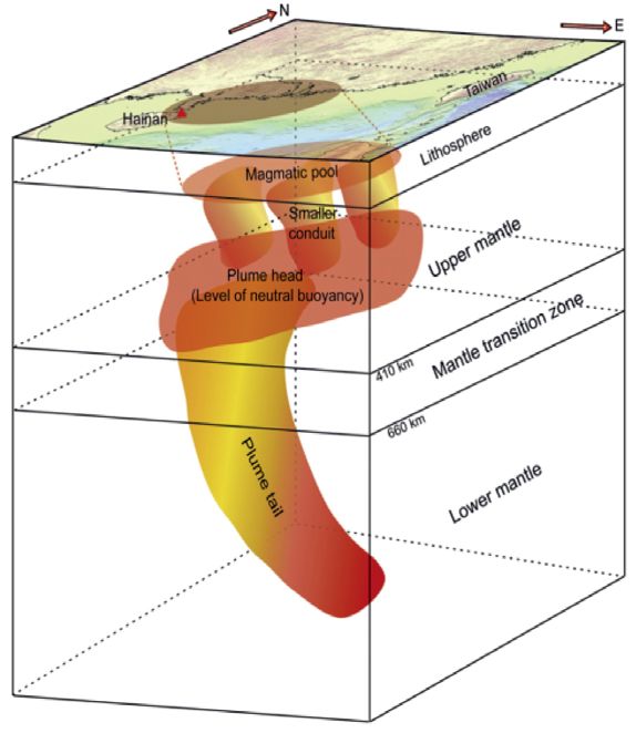
446       A. Koptev, S. Cloetingh and T.A. Ehlers

         (a)                                                                    (b)

         (c)                                                                    (d)

                                                                                                                                                                  Downloaded from https://academic.oup.com/gji/article/227/1/439/6295312 by guest on 11 September 2021
Figure 2. Design of 2-D model setup for four tested types of lithosphere: (a–c) Continental lithosphere: (a) ‘Cratonic’, (b) ‘Variscan’, (c) ‘Mesozoic’ and (d)
oceanic lithosphere (∼40 Ma old). Insets show the initial temperature distributions. A circular-shaped mantle plume anomaly is seeded just below the bottom
of the lithosphere. Lateral velocities (Vext ) are applied at vertical sides of the model.

additionally performed their thermal model analogues that exclude                  (Tinit ) and size (dinit ) of the circular thermal anomaly (mantle plume)
a kinematic component aiming to determine the purely thermal ef-                   seeded underneath unstressed (Vext : 0 mm × yr−1 ) ‘Variscan’ con-
fect of the seeded anomaly. The time span of all models with a                     tinental lithosphere.
tectonically neutral regime is 300 Myr.                                               In the first three experiments (models 1–3), the mantle plume
   In the second group of models (models 19–42), we study the                      anomaly has the same initial diameter (dinit : 100 km) whereas its
impact of external tectonic extension (Vext : 2–10 mm × yr−1 ; see                 initial temperature (Tinit ) varies from 1500 ◦ C (model 1: ‘cold’
Section 4.2). Similarly to tectonically neutral models, we first in-               plume) through 1600 ◦ C (model 2: ‘warm’ plume) to 1700 ◦ C
vestigate the case of ‘Variscan’ lithosphere (models 19–33; Section                (model 3: ‘hot’ plume), that corresponds to maximum temperature
4.2.1) which is subjected to far-field extension with a broad range                contrasts with surrounding sublithospheric mantle ( Tinit ) of ∼200,
of applied half-rates (Vext : 2, 3, 4, 5 or 10 mm × yr−1 ) also in                 ∼300 and ∼400 ◦ C, respectively.
combination with various plume temperatures (Tinit : 1500, 1600 or                    In the case of an intermediate plume temperature (model 2; Tinit :
1700 ◦ C). Finally, we explore (see Section 4.2.2) other lithospheric              1600 ◦ C), vertical and horizontal movement of the plume body
types—‘Cratonic’ (models 34–36), ‘Mesozoic’ (models 37–39) and                     results in the configuration dubbed an ‘inverted pear’ (Figs 3a
oceanic (models 40–42)—in the context of relatively slow extension                 and 4b1). Limited buoyancy contrasts in the experiment with the
(Vext : 2, 3 or 4 mm × yr−1 ) and a non-changing initial temperature of            lowest plume temperature (model 1; Tinit : 1500 ◦ C) prohibit almost
the plume (Tinit : 1600 ◦ C). Simulations of the second group models               any motion in the compositional field making indistinguishable the
have been terminated when lithospheric break-up was reached.                       modifications in the circular shape of the original mantle plume
                                                                                   which keeps its initial configuration throughout the entire mod-
                                                                                   elling time interval (Figs 4a1 and A1a). The plume material of the
4 R E S U LT S                                                                     hottest thermal anomaly (model 3; Tinit : 1700 ◦ C) first flows upwards
                                                                                   and then spreads laterally below the LAB (Figs 4c1 and A2a). As
4.1 Tectonically neutral regime (Models 1–18)                                      a result, the plume body changes its shape from an original circu-
                                                                                   lar (Fig. 2b) into a heart-like configuration (Fig. A2a; time slice
4.1.1 Effect of initial plume temperature and diameter (models                     of 15 Myr). Subsequently, the latter evolves into a quasi-elliptical
1–9)                                                                               form with an aspect ratio of vertical height (dver ) to horizontal length
As mentioned above, we start our modelling with a series of ex-                    (dhor ) of ∼1:2 (Figs 4c1 and A2a; time slices of ≥60 Myr). Note that
periments aimed to explore the variations in initial temperature                   in both models 2 and 3, the final figure of the plume is established at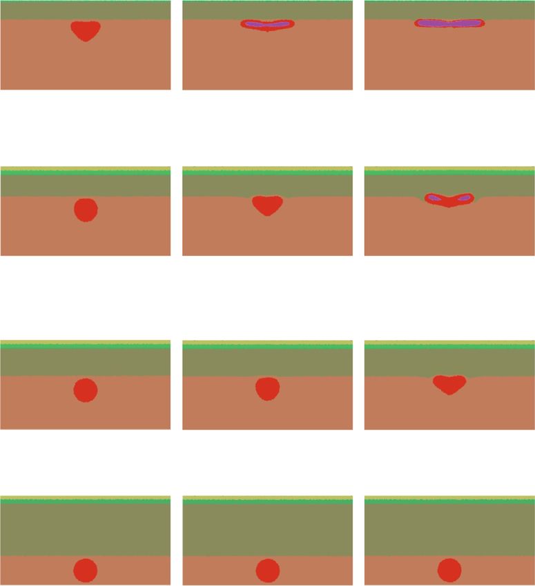
‘Baby’ plumes and break-up            447

Table 2. Controlling parameters of the numerical experiments.
                                            Controlling parameters
                        Plume properties
             Temperature, Tinit    Diameter, dinit      Type of lithosphere     Extension half-rate,
                 [◦ C]                  [km]                                   Vext [mm × yr−1 ]                  Figure                Section
1                  1500                   100                    ‘Variscan’             0               A1, 4, 5, A3, 9, 11, 12, A10       4.1.1
2                  1600                   100                    ‘Variscan’              0              3, 4, 5, 6, 9, 10, 11, 12, A11
3                  1700                   100                    ‘Variscan’              0              A2, 4, 5, A4, 9, 11, 12, A12
4                  1500                   80                     ‘Variscan’             0                            A3, 9
5                  1600                   80                     ‘Variscan’             0                             6, 9
6                  1700                   80                     ‘Variscan’             0                            A4, 9
7                  1500                   116                    ‘Variscan’             0                            A3, 9
8                  1600                   116                    ‘Variscan’              0                            6, 9
9                  1700                   116                    ‘Variscan’             0                         A4, 7, 8, 9
10                 1500                   100                    ‘Cratonic’             0                         A5, 11, 12               4.1.2

                                                                                                                                                       Downloaded from https://academic.oup.com/gji/article/227/1/439/6295312 by guest on 11 September 2021
11                 1600                   100                    ‘Cratonic’             0                       A5, 10, 11, 12
12                 1700                   100                    ‘Cratonic’             0                         A5, 11, 12
13                 1500                   100                   ‘Mesozoic’               0                        A6, 11, 12
14                 1600                   100                   ‘Mesozoic’               0                      A6, 10, 11, 12
15                 1700                   100                   ‘Mesozoic’               0                        A6, 11, 12
16                 1500                   100                     oceanic               0                         A7, 11, 12
17                 1600                   100                     oceanic               0                       A7, 10, 11, 12
18                 1700                   100                     oceanic               0                         A7, 11, 12
19                 1500                   100                    ‘Variscan’             2                        A8, A10, 14               4.2.1
20                 1600                   100                    ‘Variscan’              2                   13, A11, 14, 15, 16
21                 1700                   100                    ‘Variscan’              2                       A9, A12, 14
22                 1500                   100                    ‘Variscan’              3                          A10, 14
23                 1600                   100                    ‘Variscan’              3                        A11, 14, 16
24                 1700                   100                    ‘Variscan’              3                          A12, 14
25                 1500                   100                    ‘Variscan’              4                             14
26                 1600                   100                    ‘Variscan’              4                           14, 16
27                 1700                   100                    ‘Variscan’              4                             14
28                 1500                   100                    ‘Variscan’              5                             14
29                 1600                   100                    ‘Variscan’              5                           14, 16
30                 1700                   100                    ‘Variscan’              5                             14
31                 1500                   100                    ‘Variscan’             10                             14
32                 1600                   100                    ‘Variscan’             10                           14, 16
33                 1700                   100                    ‘Variscan’             10                             14
34                 1600                   100                    ‘Cratonic’             2                            15, 16                4.2.2
35                 1600                   100                    ‘Cratonic’             3                              16
36                 1600                   100                    ‘Cratonic’             4                              16
37                 1600                   100                   ‘Mesozoic’               2                           15, 16
38                 1600                   100                   ‘Mesozoic’              3                              16
39                 1600                   100                   ‘Mesozoic’              4                              16
40                 1600                   100                     oceanic               2                            15, 16
41                 1600                   100                     oceanic               3                              16
42                 1600                   100                     oceanic               4                              16
Note: The depths of Moho and LAB for different types of lithosphere: ‘Cratonic’ (Moho: 36 km, LAB: 250 km); ‘Variscan’ (Moho: 36 km, LAB: 150 km);
‘Mesozoic’ (Moho: 36 km, LAB: 125 km); oceanic (Moho: 8 km, LAB: 80 km). See Section 3 for more detail.

∼50–60 Myr after model onset without subsequent changes (Figs 3a              fields (T ) after several tens to 100 Myr (see Figs 3b, A1b and A2b).
and A2a).                                                                     In order to illustrate in more detail the evolution of explored plume-
   The presence of the thermal anomaly seeded just below the litho-           related thermal anomalies, we compute the temperature contrast
spheric bottom leads to upward deflection of the 1300 ◦ C isotherm            ( T ) defined as the difference between the current temperature in
by several tens of km (e.g. model 2; Fig. 3b) This deflection not             the corresponding grid node and the temperature from the near-
only remains discernible over the whole time span of all models (in-          edge column taken at the same vertical level. Distributions of the
cluding the experiment with the ‘cold’ mantle plume—see model 1               temperature contrast ( T ) are calculated for each time step (see
in Figs 4a2 and A1b) but also appears to be more pronounced (in               Figs 3c and 4, lower row; Figs A1c and A2c) allowing to explore
terms of both width and amplitude; Figs 4c2 and A2b) when the                 the evolution of plume-induced thermal disturbances in space and
plume is ‘hot’ (model 3; Tinit : 1700 ◦ C). In the latter case a stronger     time with the following parameters (Fig. 5):
thermal impact is accompanied by a mechanical component of the
vertical uplift combined with horizontal propagation of the plume
material underneath the lithosphere (Figs 4c1 and A2a).
   However, regardless the adopted initial temperature Tinit the man-            1) Maximum temperature contrast detected over the entire mod-
tle plumes themselves become almost invisible in the temperature              elling area at the current time step ( Tmax );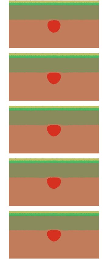
448       A. Koptev, S. Cloetingh and T.A. Ehlers

             (a)                                         (b)                                           (c)

                                                                                                                                                                    Downloaded from https://academic.oup.com/gji/article/227/1/439/6295312 by guest on 11 September 2021
Figure 3. Temporal evolution of model 2 (Tinit : 1600 ◦ C; dinit : 100 km; type of lithosphere: ‘Variscan’; Vext : 0 mm × yr−1 ): (a) material phase field. Since
60 Myr the plume has an inverted pear (or a light bulb) shape; (b) distribution of the temperatures (T ) and (c) temperature contrasts ( T ). The areas A x and
corresponding wx are shown in the panel ‘c’ for the following T thresholds: x = 200, 100, 75 and 50 ◦ C.

   2) Maximum horizontal extent or width (wx ) of the area (A x )                   below the reference temperature values (e.g. 200, 100 or 75 ◦ C)
characterized by a temperature contrast ( T ) higher than a prede-                  appear to vary over a wide range from one experiment to another.
fined threshold value (x). We present here wx estimated for A x                     In particular, the difference in the timing of cooling below 100 ◦ C
corresponding to x = 300, 200, 100, 75 and 50 ◦ C (i.e. w300 ,                      between ‘cold’ plume model 1 (Tinit : 1500 ◦ C) and ‘hot’ plume
w200 , w100 , w75 and w50 , respectively). Examples of areas A x de-                model 3 (Tinit : 1700 ◦ C) is exceeding 100 Myr.
fined for various x as well as corresponding wx are illustrated in                     The temporal evolution of w100 (horizontal width of the plume
Fig. 3c;                                                                            segment where Tmax remains higher than 100 ◦ C) also significantly
                                            int
   3) Temperature contrast integral  ( Tx ) taken over the area A x                differs within these models (Fig. 5, middle row). The ‘cold’ model
(see above) as follow: Tx = Ax T d A x . Similar to wx , we
                              int
                                                                                    1 shows a quick decrease of w100 in a quasi-parabolic manner from
estimate five values of Txint : T300   int      int
                                           , T200       int
                                                    , T100  , T75int and            initial 100 km (at 0 Myr) to 0 km at ∼55 Myr. On the contrary, w100
     int
   T50 .                                                                            of the ‘warm’ experiment (model 2) remains close to the original
                                                                                    value of 100 km over the first ∼60 Myr before its parabolic drop to
  As mentioned above, the initial maximum temperature contrast                      zero during the following ∼65 Myr. As mentioned above, the ‘hot’
( Tmax at 0 Myr or Tinit ) varies from of ∼200 to ∼400 ◦ C de-                      plume anomaly (model 3; Tinit : 1700 ◦ C) flattens below the LAB
pending on the initial plume temperature (Tinit ). In all experiments,              thus subjecting the originally circular plume to significant horizontal
  Tmax decreases quickly during the first ∼50–100 Myr after that                    stretching (Fig. 4c1). As a result, at the early stage of evolution w100
cooling slows down (Fig. 5, upper row). Although all curves of                      becomes wider than its initial value of 100 km reaching ∼150 km at
  Tmax look at first sight similar, the time points when they descent               ∼20–60 Myr whereas its subsequent quasi-parabolic descent lasts
‘Baby’ plumes and break-up 449
(a) (b) (c)
Downloaded from https://academic.oup.com/gji/article/227/1/439/6295312 by guest on 11 September 2021
Figure 4. (a) Model 1 (Tinit : 1500 ◦ C; ∗ ); (b) model 2 (Tinit : 1600 ◦ C; ∗ ) and (c) model 3 (Tinit : 1700 ◦ C; ∗ ) represented by (1) material phase field (upper row);
(2) distribution of the temperatures (T ; middle row); (3) temperature contrasts ( T ; lower row) at the time slice of 60 Myr. ∗ Other experimental parameters:
dinit : 100 km; type of lithosphere: ‘Variscan’; Vext : 0 mm × yr−1 .
more than a hundred Myr (∼130 Myr, i.e. >2 time longer than in star in Fig. 5a3). This initial Txint corresponds to an integrated
models 1 and 2) ending at ∼190 Myr. value of plume buoyancy of ∼1.2 × 10¹¹ kg × m−1 . In the models
Given that a temperature contrast of 100 ◦ C is close to the min- 2 (Tinit : 1600 ◦ C) and 3 (Tinit : 1700 ◦ C), Txint for x = 100 ◦ C
imum T value detectable by seismic tomography imaging (e.g. (i.e. T100 int
) decreases to the same value (∼1.2 × 10¹² ◦ C × m2 ) at
Cammarano et al. 2003), we exploit w100 to identify quantitatively ∼35 and ∼95 Myr, respectively (see grey stars in Figs 5b3 and c3).
the moment in time when the plume evolution enters into the termi- Note also that the values of w100 corresponding to these time points
nal phase. For this purpose, we introduce a new parameter t(w100 50
) (∼35 and ∼95 Myr) in these experiments (models 2 and 3) are close
which refers to the time point when w100 subsides below 50 km to or even slightly exceed the initial dinit of 100 km. Therefore, it
(i.e. half of original w100 ; Fig. 5b2), thus approaching the resolution appears that the evolution of ‘warm’ (model 2; Tinit : 1600 ◦ C) and
limit of modern seismic tomography (e.g. Rickers et al. 2013; Plom- ‘hot’ (model 3; Tinit : 1700 ◦ C) mantle plumes is characterized by
50
erová et al. 2016). While t(w100 ) characterizes a ‘decay time’ of the time intervals of tens to 100 Myr when the sum temperature excess
thermal anomaly, a plume ‘lifespan’ corresponds to the time period concentrated within the area of a seismically detectable thermal
between model onset (0 Myr) and t(w100 50
). Despite the extremely anomaly ( T >100 ◦ C; w100 ≥100 km) remains higher or roughly
small size (dinit : 100 km) of the ‘baby’ plumes explored here, their equal to the original (i.e. at 0 Myr) temperature contrast integrated
lifespan appears to cover long time intervals varying from ∼40 Myr over the surface of a ‘cold’ mantle plume (model 1; Tinit : 1500 ◦ C).
(model 1; Tinit : 1500 ◦ C) through ∼110 Myr (model 2; Tinit : 1600 In order to investigate the role of initial plume size we performed
◦
C) to ∼170 Myr (model 3; Tinit : 1700 ◦ C). the models with different dinit : 80 km (models 4–6) and 116 km
Graphs of integrated temperature contrasts ( Txint ) for the mod- (models 7–9). The values of 80 and 116 km are chosen to ensure
els 1–3 are summarized in the lower row of Fig. 5. The quasi- that variations in the initial plume area are by a factor of ∼2 between
parabolic reduction of each Txint during the first ∼20–30 Myr is the smallest and largest end-members: given that A = π4d , A(Tinit
2
faster than their subsequent quasi-linear decrease. Expectedly, the = 116 km) ≈ 2×A(Tinit = 80 km) because 1162 ≈ 2 × 802 .
steepness of both non-linear and linear trends of Txint evolution is For intermediate temperature (Tinit : 1600 ◦ C), variations in the
mainly controlled by the T threshold limit (i.e. x) which defines initial diameter (dinit : 80, 100 or 116 km) of the plume anomaly
integrating area A x for each Txint (see above): higher x values re- appear to have a similar effect to that of initial temperature changes
sult in a steeper decrease of Txint . On the contrary, the initial value (Tinit : 1500, 1600 or 1700 ◦ C) in the ‘standard’ diameter (dinit :
of Txint (i.e. Txint at 0 Myr) is independent from x because an 100 km) models (compare Figs 5 and 6). A plume with a reduced
original A x coincides with the circular area of the imposed thermal initial diameter (dinit : 80 km) starts to decay ∼55 Myr earlier (at
anomaly for all tested T threshold limits (i.e. x) that are lower than ∼55 Myr) than in the standard (dinit : 100 km) case (∼110 Myr)—
Tinit (i.e. Tmax at 0 Myr). Thus, the initial Txint in the model 1 see decay time t(w100 50
) indicated in Figs 6a2 and b2, respectively.
(Tinit : 1500 ◦ C) is ∼1.2 × 10¹² ◦ C × m2 for all x ≤ 100 ◦ C (see grey On the contrary, an increased diameter (dinit : 116 km) extends theYou can also read


