Autotuning Hamiltonian Monte Carlo for efficient generalized nullspace exploration
←
→
Page content transcription
If your browser does not render page correctly, please read the page content below
Geophys. J. Int. (2021) 227, 941–968                                                                                  https://doi.org/10.1093/gji/ggab270
Advance Access publication 2021 July 15
GJI Seismology

Autotuning Hamiltonian Monte Carlo for efficient generalized
nullspace exploration

Andreas Fichtner , Andrea Zunino, Lars Gebraad and Christian Boehm
Department of Earth Sciences, ETH Zurich, Sonneggstrasse 5, 8092 Zurich, Switzerland. E-mail: andreas.fichtner@erdw.ethz.ch

Accepted 2021 July 13. Received 2021 May 7; in original form 2020 December 14

                                                                                                                                                            Downloaded from https://academic.oup.com/gji/article/227/2/941/6321848 by guest on 28 August 2021
                                       SUMMARY
                                       We propose methods to efficiently explore the generalized nullspace of (non-linear) inverse
                                       problems, defined as the set of plausible models that explain observations within some misfit
                                       tolerance. Owing to the random nature of observational errors, the generalized nullspace is
                                       an inherently probabilistic entity, described by a joint probability density of tolerance val-
                                       ues and model parameters. Our exploration methods rest on the construction of artificial
                                       Hamiltonian systems, where models are treated as high-dimensional particles moving along a
                                       trajectory through model space. In the special case where the distribution of misfit tolerances
                                       is Gaussian, the methods are identical to standard Hamiltonian Monte Carlo, revealing that its
                                       apparently meaningless momentum variable plays the intuitive role of a directional tolerance.
                                       Its direction points from the current towards a new acceptable model, and its magnitude is
                                       the corresponding misfit increase. We address the fundamental problem of producing inde-
                                       pendent plausible models within a high-dimensional generalized nullspace by autotuning the
                                       mass matrix of the Hamiltonian system. The approach rests on a factorized and sequentially
                                       preconditioned version of the L-BFGS method, which produces local Hessian approximations
                                       for use as a near-optimal mass matrix. An adaptive time stepping algorithm for the numerical
                                       solution of Hamilton’s equations ensures both stability and reasonable acceptance rates of
                                       the generalized nullspace sampler. In addition to the basic method, we propose variations of
                                       it, where autotuning focuses either on the diagonal elements of the mass matrix or on the
                                       macroscopic (long-range) properties of the generalized nullspace distribution. We quantify
                                       the performance of our methods in a series of numerical experiments, involving analytical,
                                       high-dimensional, multimodal test functions. These are designed to mimic realistic inverse
                                       problems, where sensitivity to different model parameters varies widely, and where parameters
                                       tend to be correlated. The tests indicate that the effective sample size may increase by orders
                                       of magnitude when autotuning is used. Finally, we present a proof of principle of generalized
                                       nullspace exploration in viscoelastic full-waveform inversion. In this context, we demonstrate
                                       (1) the quantification of inter- and intraparameter trade-offs, (2) the flexibility to change model
                                       parametrization a posteriori, for instance, to adapt averaging length scales, (3) the ability to
                                       perform dehomogenization to retrieve plausible subwavelength models and (4) the extraction
                                       of a manageable number of alternative models, potentially located in distinct local minima of
                                       the misfit functional.
                                       Key words: Inverse theory; Numerical solutions; Probability distributions; Statistical meth-
                                       ods; Seismic tomography.

                                                                                Imperfections of these data combined with inherent (physical) non-
1 I N T RO D U C T I O N
                                                                                uniqueness and unavoidable simplifications of the equations render
Our knowledge about the internal structure of bodies that are inac-             the solution of any inverse problem ambiguous. Actually solving an
cessible to direct observation, such as the Earth or the human body,            inverse problem therefore requires us to describe the ‘very infinite-
derives from the solution of inverse problems, which assimilate data            dimensional’ manifold of ‘acceptable models’ (Backus & Gilbert
to constrain the parameters m of some forward modelling equations.              1968), that is, models with a misfit χ (m) below some threshold.


C The Author(s) 2021. Published by Oxford University Press on behalf of The Royal Astronomical Society. This is an Open Access

article distributed under the terms of the Creative Commons Attribution License (http://creativecommons.org/licenses/by/4.0/), which
permits unrestricted reuse, distribution, and reproduction in any medium, provided the original work is properly cited.
                                                                                                                                                     941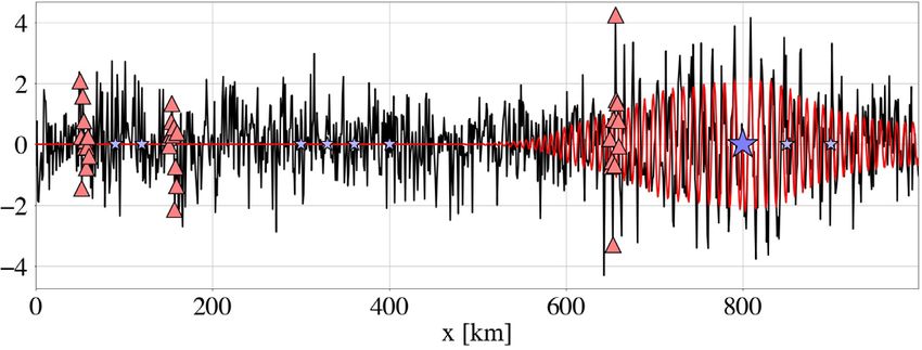
942      A. Fichtner et al.

1.1 Characterizing acceptable solution- and nullspace                      In addition to providing independent models at minimal cost, a
                                                                        generalized nullspace sampler should be adaptable to the needs
Trying to tame the intimidating infinite-dimensionality of the so-
                                                                        of a specific application. In particular, taking a data-oriented
lution space, Backus & Gilbert themselves formalized a series of
                                                                        perspective, it should enable a flexible notion of what makes a
approaches that were to be used for decades to come. These include
                                                                        model acceptable. If, for instance, a currently available model
the linearization of the forward modelling equations, an expansion
                                                                        m0 produces a rather large misfit χ (m0 ), other models may be
of plausible solutions into a finite number of orthogonal basis func-
                                                                        required to have a generally lower misfit in order to be accept-
tions, the computation of parameter averages using optimally δ-like
                                                                        able. Alternatively, models may be acceptable when their associ-
averaging kernels and the solution of constrained least-squares prob-
                                                                        ated misfits fall within a range controlled by the observational error
lems (Backus & Gilbert 1967, 1968, 1970). For the special case of
                                                                        statistics.
linear problems, Wiggins (1972) analysed that part of model space
                                                                           From a model-oriented perspective, a generalized nullspace sam-
for which error-contaminated data provide only weak constraints.
                                                                        pler should have the flexibility to preferentially explore models
He then proposed to construct what would today be called the gener-
                                                                        with predefined and application-specific characteristics. We may,
alized nullspace using singular-value decomposition. Modern vari-
                                                                        for example, be interested in alternative models that contain more
ants of Wiggins’ concept, adapted to higher-dimensional model-
                                                                        small-scale structure or are smoother than our current model m0 .
and nullspaces, can be found in Deal & Nolet (1996) and de Wit
                                                                        Similarly, in the context of quantitative hypothesis testing, we may

                                                                                                                                                  Downloaded from https://academic.oup.com/gji/article/227/2/941/6321848 by guest on 28 August 2021
et al. (2012) for linear problems, and in Liu & Peter (2020) for
                                                                        want to find alternative models that contain specific new features to
problems that can be linearized reasonably well.
                                                                        an extent that is compatible with previously assimilated data.
   Efforts, such as the one of Kennett (1978), to characterize the
space of acceptable solutions (or, equivalently, the generalized
nullspace) for non-linear inverse problems have remained few in
number. Instead, increasing computational power enabled Monte           1.3 Outline
Carlo methods, adapted from statistical physics (Metropolis et al.
                                                                        Based on these challenges and desiderata, this manuscript is orga-
1953; Metropolis 1987), to provide finite sets of acceptable mod-
                                                                        nized as follows. In Section 2, we define the generalized nullspace
els by brute-force forward modelling and testing against data (e.g.
                                                                        in terms of a misfit tolerance, which, by virtue of random observa-
Keilis-Borok & Yanovskaya 1967; Press 1968, 1970).
                                                                        tional errors, is a probabilistic quantity. Subsequently, we demon-
   Concerns how to quantitatively digest the potentially large en-
                                                                        strate that the generalized nullspace can be explored using a me-
semble of acceptable models produced by Monte Carlo sampling
                                                                        chanical analogue, whereby model is treated as a particle on a
(e.g. Anderssen & Seneta 1971; Kennett & Nolet 1978) dispersed
                                                                        trajectory controlled by Hamilton’s equations. The classical HMC
with the realization that they may be used to properly sample the
                                                                        algorithm (e.g. Duane et al. 1987; Neal 2011) emerges from this
posterior probability density ρ(m) ∝ e−χ (m) , which in turn could
                                                                        analysis as the special case where the misfit tolerances follow a chi-
be related to a rigorous application of Bayes’ theorem (Mosegaard
                                                                        squared distribution. Via a series of examples we will see that the
& Tarantola 1995). From the samples one may select some that
                                                                        efficiency of the generalized nullspace sampler critically depends
fall within the generalized nullspace, or one may compute lower-
                                                                        on its tuning, and specifically on the artificial mass matrix of the
dimensional quantities, such as means, marginal distributions or
                                                                        particle.
(higher-order) moments.
                                                                           Within this context, Section 3 proposes an autotuning mecha-
   What followed was the development of numerous Monte Carlo
                                                                        nisms. This involves (1) an on-the-fly quasi-Newton approximation
variants that go beyond the classic Metropolis–Hastings algorithm
                                                                        of the misfit Hessian which serves as near-optimal mass matrix
(Hastings 1970) in trying to adapt to the particularities of high-
                                                                        and (2) an adaptive time-stepping approach that ensures stability of
dimensional, non-linear inverse problems. These methods include,
                                                                        the numerical solution of Hamilton’s equations as the mass matrix
but are not limited to, parallel tempering (e.g. Geyer & Thompson
                                                                        changes.
1995; Sambridge 2014), the Neighbourhood Algorithm (Sambridge
                                                                           Section 4 is dedicated to a performance assessment of the pro-
1999a,b), the reversible-jump algorithm used for transdimensional
                                                                        posed autotuning method and some of its variants. For this, we
inversion (e.g. Green 1995; Sambridge et al. 2006, 2013), Hamil-
                                                                        consider high-dimensional and strongly multimodal analytical test
tonian Monte Carlo (HMC, e.g. Duane et al. 1987; Sen & Biswas
                                                                        functions with significant parameter correlations, that are designed
2017; Fichtner et al. 2019) or the Metropolis-adjusted Langevin
                                                                        to mimic misfit surfaces that one may encounter in realistic inverse
algorithm (MALA, e.g. Roberts & Tweedie 1996; Izzatullah et al.
                                                                        problems. In these examples, autotuning helps to reduce the number
2021).
                                                                        of samples needed to achieve convergence by more than one order
                                                                        of magnitude.
                                                                           Encouraged by these results, Section 5 presents a generalized
1.2 Challenges and desiderata
                                                                        nullspace exploration for 1-D viscoelastic full-waveform inversion,
Despite undeniable progress, challenges remain. Arguably the most       which enables, for example, the detection of different misfit minima.
important among these is the efficient computation of acceptable        The ability to treat high-dimensional models spaces allows us to
models that are independent, that is, significantly different from      parametrize the model at subwavelength scale, and to choose some
each other. As the model space dimension Nm grows, the proba-           spatial parameter averaging a posteriori, for instance, as a function
bility of completely randomly drawing a model m that happens to         of the desired certainty. Furthermore, we propose an algorithm that
be acceptable, decreases superexponentially (e.g. Tarantola 2005;       extracts a manageable number of acceptable models that are at a
Fichtner 2021). Increasing the acceptance rate of trial models may      predefined minimum distance from each other.
require very small steps from the current model to a new candidate         Finally, in Section 6, we discuss, among other aspects, the relation
model, which leads to both an explosion of computational cost and       of our method to (1) previous work in Hessian-aware Monte Carlo
slow convergence of the sample chain (e.g. Geyer 1992; Krass et al.     sampling, (2) dehomogenization and the construction of alternative
1998; MacKay 2003; Gelman et al. 2013).                                 small-scale models and (3) non-linear full-waveform inversion.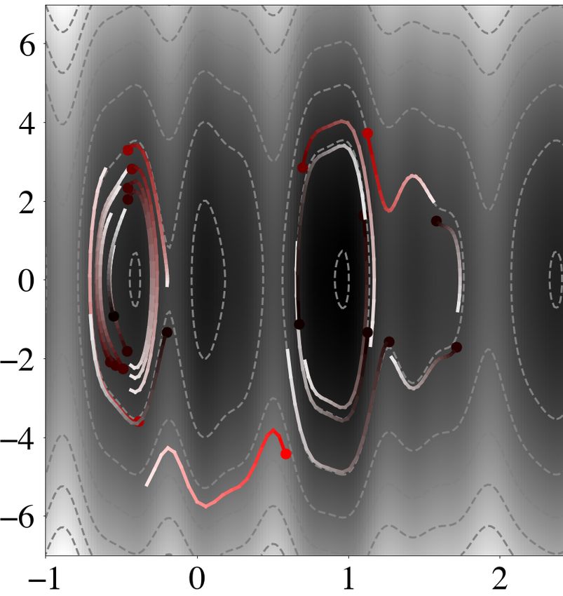
Autotuning HMC for nullspace exploration                943

2 R A N D O M I Z E D N U L L S PA C E                                     When p0 is chosen such that
E X P L O R AT I O N
                                                                                       1 T −1
We begin with the notion of a generalized nullspace. For this we           K (p0 ) =    p M p0 = ε,                                             (6)
                                                                                       2 0
assume the existence of an estimated plausible model m0 with misfit
χ0 = χ (m0 ), which approximately minimizes the misfit functional          Eq. (6) implies
χ . The estimate may have been found using gradient-based (e.g.
Nocedal & Wright 1999) or stochastic (e.g. Sen & Stoffa 2013;              χ [m(τ )] ≤ χ (m0 ) + ε,                                             (7)
Fichtner 2021) methods, or it may represent a priori knowledge
                                                                           because the positive definiteness of the mass matrix M ensures
from previous analyses. Due to observational uncertainties, forward
                                                                           p(τ )T M−1 p(τ ) > 0 for all momenta p(τ ). Consequently, all models
modelling errors and inherent non-uniqueness, alternative models,
                                                                           m(τ ) along the trajectory are within the generalized nullspace.
m0 + m, are still plausible when the associated misfit increase
                                                                              While the Hamiltonian system constructed for nullspace explo-
remains below some tolerance ε ≥ 0, that is,
                                                                           ration seems artificial, eq. (6) injects concrete physical meaning into
χ (m0 + m) ≤ χ0 + ε.                                               (1)    the momentum variable p. In fact, p0 plays the role of an initial di-
                                                                           rectional tolerance. Its M−1 -norm ||p0 ||2M = 12 p0T M−1 p0 determines
The ensemble of tolerable models m0 + m constitutes the gener-            the maximum admissible misfit increase, and its direction controls

                                                                                                                                                       Downloaded from https://academic.oup.com/gji/article/227/2/941/6321848 by guest on 28 August 2021
alized nullspace (Deal & Nolet 1996).                                      the initial direction in model space along which alternative models
                                                                           are sought. In fact, as shown in Fichtner & Zunino (2019), the model
                                                                           perturbation applied by the nullspace shuttle during the initial and
2.1 Hamiltonian nullspace shuttle                                          infinitesimally short part of its trajectory is proportional to M−1 p0 .
                                                                           Hence, p0 may be used to insert specific features into alternative
For a given tolerance ε, generalized nullspace exploration can
                                                                           models. The mass matrix may then modify these features, making
be achieved through the interpretation of a model m as the Nm -
                                                                           them, for example, rougher or smoother. Hamilton’s eq. (4) govern
dimensional position vector of an imaginary particle, also referred
                                                                           the change of the directional tolerance, from the initial p0 to some
to as the nullspace shuttle (Fichtner & Zunino 2019; Fichtner 2021).
                                                                           p(τ ).
The position of the particle varies as a function of an artificially in-
troduced time τ , meaning that different τ correspond to different
members of model space, m(τ ). To determine the movement of the
particle through model space, we construct artificial equations of
motion, borrowing concepts from classical mechanics (e.g. Symon            2.2 The probabilistic generalized nullspace
1971; Landau & Lifshitz 1976). First, we equate the (not necessarily
                                                                           Random errors in the observed data vector dobs cause the generalized
positive definite) misfit χ (m) with an artificial potential energy of
                                                                           nullspace to be an inherently probabilistic entity. The repetition of
the particle,
                                                                           the experiment, in reality or hypothetically, would yield a different
U (m) = χ (m).                                                      (2)    realization of dobs and a different misfit χ 0 . Hence, for a given m0
                                                                           the distribution of misfits is characterized by a probability density
The potential energy, most intuitively imagined as a gravitational         ρ(χ |m0 ). The random nature of χ translates to the tolerance ε. Had
energy, induces a force −∇U [m(τ )], parallel to the direction of          we, for instance, obtained a smaller misfit for m0 by chance, we
steepest descent. Hence, within some time increment δτ , the po-           would possibly accept a larger tolerance, and vice versa. Therefore,
tential energy acts to move m(τ ) towards a new model m(τ + δτ )           we may equally describe the distribution of ε by a probability density
with lower misfit. The ‘gravitational’ force parallel to −∇U [m(τ )]       ρ(ε|m0 ).
is complemented by an inertial force, related to an artificial momen-         The directional tolerance p0 inherits the probabilistic character
tum p(τ ), which also has dimension Nm . Together with an equally          of the scalar tolerance ε, but its distribution ρ(p0 |m0 ) is not solely
artificial, symmetric and positive-definite mass matrix M, the mo-         controlled by the misfit statistics. In fact, considering eq. (6), we
mentum defines the kinetic energy                                          may obtain some p0 for a specific realization of ε by (1) drawing a
          1 T −1                                                           vector q from an arbitrary probability distribution, (2) rescaling q
K (p) =     p M p.                                                  (3)    such that qT q = 2ε and (3) setting p0 = Sq, where M = SST is a
          2
                                                                           factorization of the mass matrix. Clearly, the vector p0 , intuitively
The sum of potential and kinetic energies, that is, the total energy       interpretable as the initial take-off direction of the nullspace shuttle,
of the artificial mechanical system, is the Hamiltonian H (m, p) =         depends on the mass matrix M, which we are free to choose, as long
U (m) + K (p). In terms of H, the trajectory of the Nm -dimensional        as it is symmetric and positive definite.
particle is fully determined by Hamilton’s equations                          As schematically illustrated in Fig. 1, the design of M can be
dm i   ∂H           d pi    ∂H                                             used to introduce additional information or desiderata about the di-
     =      ,            =−      ,        i = 1, ..., Nm .          (4)    rection along which alternative models should be found. This may
dτ     ∂ pi         dτ      ∂m i
                                                                           include average properties of the take-off directions, subjective pref-
Along any trajectory in phase (model-momentum) space, H is pre-            erences, or the need to incorporate new, independent information
served. Hence, starting at some approximate minimum m0 of χ and            into a model without deteriorating the fit to previously included
some initial momentum p0 , the solution of eq. (4) leads to a contin-      data. The precise meaning of the generalized nullspace depends
uous sequence of models m(τ ) and momenta p(τ ) that satisfy               on how we construct M and therefore ρ(p0 |m0 ). To avoid overly
                              1                                            abstract developments, we will present application-specific exam-
H [m(τ ), p(τ )] = χ [m(τ )] + p(τ )T M−1 p(τ ) = H (m0 , p0 )             ples of ρ(p0 |m0 ) throughout the following sections. An expanded
                              2
                                                                           collection of possible tolerance distributions, including the special
                        1 T −1
                 = χ 0 + p0 M p 0 .                                 (5)    case of zero tolerance, can be found in Appendix A.
                        2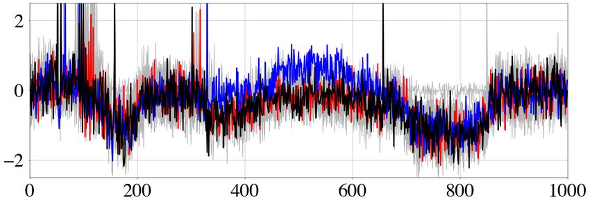
944         A. Fichtner et al.

  (a) statistically isotropic p0   (M=I)                (b) statistically anisotropic p0   (M I)                    (c) objectively/subjectively biased p0

                                                                                                                                                       feature X
                                                                                                                                     smoother         suppressed

                                           p0                                                         p0              preferred by                                   p0
                                                                                                                         myself

                                                                                                                      sharper
                                                                                                                       edges                                           preferred by
                                                                                                                                                                         my boss

                                                                                                                         feature X                                 rougher
                                                                                                                         enhanced

                                                                                                                                                     consistent with new
                                                                                                                                                   independent information

Figure 1. Schematic illustration of the probability distribution for directional tolerances ρ(p0 |m0 ) as a function of the mass matrix M. The radius of the pale

                                                                                                                                                                                        Downloaded from https://academic.oup.com/gji/article/227/2/941/6321848 by guest on 28 August 2021
dashed circle equals a specific realization of the scalar tolerance ε, and the blue arrow marks a specific p0 , which can be interpreted as the initial take-off
direction of the nullspace shuttle. (a) When M = I, the distribution of initial momenta is isotropic. (b) For M = I, certain directions will be preferred, meaning
that the distribution is statistically anisotropic. (c) The mass matrix M may also be designed to favour specific directions that are in accord with personal
preference or new independent information.

  The product of the tolerance distribution ρ(p|m) and the model                             2021), which recently gained attention in geophysics for its abil-
space posterior ρ(m),                                                                        ity to solve inverse problems of comparatively high dimension (e.g.
                                                                                             Sen & Biswas 2017; Fichtner & Simute 2018; Fichtner et al. 2019;
ρ(p, m) = ρ(p|m)ρ(m),                                                         (8)
                                                                                             Gebraad et al. 2020; Kotsi et al. 2020; Muir & Tkalčić 2020). In
defines a joint probability density in tolerance-model space. This                           HMC, scalar tolerances ε are drawn from a chi-squared distribu-
generalized nullspace distribution describes the combined informa-                           tion with n degrees of freedom, independent of the current model
tion on alternative models and misfit tolerances that we are willing                         mi . This means that acceptable misfit increases scale with model
to accept. For a fixed directional tolerance p, the joint distribution                       space dimension (Appendix A3). The corresponding distribution
ρ(p, m) provides the likelihoods of acceptable models. Conversely,                           of the directional tolerances pi is the Nm -dimensional Gaussian
for a fixed model m, it gives the likelihood of accepting a certain                          with covariance matrix M, also independent of the current posi-
misfit increase. Finally, integrating (marginalizing) ρ(p, m) over the                       tion mi in model space. A conceptual difference between Hamilto-
tolerances p, returns the model space posterior ρ(m).                                        nian nullspace sampling and HMC is the initial model m0 . While
                                                                                             nullspace sampling assumes that m0 is already an acceptable model,
                                                                                             m0 is drawn randomly in HMC. After sufficiently many samples, the
2.3 Sampling the generalized nullspace distribution                                          influence of the initial model will diminish, and so this difference
                                                                                             disappears asymptotically. Yet, as noted by Geyer (2011), Monte
For problems of sufficiently low dimension, the complete joint dis-
                                                                                             Carlo methods in general benefit from choosing an acceptable m0 ,
tribution ρ(p, m) may be explored by brute-force grid search. How-
                                                                                             as this may eliminate or at least shorten the burn-in phase, which is
ever, when the model space dimension is high, that is, typically
                                                                                             otherwise needed to approach the typical set.
above a few tens or hundreds, we typically need to limit ourselves
                                                                                                In many applications, Hamilton’s equations cannot be integrated
to the Monte Carlo approximation of lower-dimensional quantities.
                                                                                             analytically, meaning that numerical integrators must be used to
These may include moments of the distribution (means, variances,
                                                                                             obtain approximate solutions. While the numerical approximation
...), marginal probability densities, or other lower-dimensional char-
                                                                                             may affect the conservation of energy, the sampling algorithm pre-
acteristics of the posterior.
                                                                                             sented above remains valid as long as the numerical integrator is
    As proven in Appendix B, the Hamiltonian nullspace exploration
                                                                                             symplectic, that is, time-reversible and volume-preserving (see Ap-
described in Section 2.1 provides a mechanism for the Monte Carlo
                                                                                             pendix B).
sampling of ρ(p, m), which we summarize in the following algo-
rithm:
   (1) Starting from m0 , randomly draw a directional tolerance p0                           2.4 Examples
from ρ(p|m0 ).
   (2) Propagate (p0 , m0 ) for some time T along a Hamiltonian                              2.4.1 The 1-D harmonic oscillator
trajectory towards the test momentum/model (p(T ), m(T )).                                   For the purpose of illustration, we begin with the simple example
   (3) Accept         (p(T ), m(T ))       with        probability                           of inferring the circular frequency m of a 1-D harmonic oscillator
min [1, ρ(p(T ), m(T ))/ρ(p0 , m0 )] .                                                       from observations of its amplitude
   In case of acceptance, set m(T ) → m1 and repeat the proce-                               u(t) = 1.2 sin(mt),                                                                  (9)
dure by drawing p1 according to step 1). Otherwise, continue
with m0 retry the procedure, as before. The resulting Markov                                 at few irregularly spaced observations times t1 , ..., t Nd , as illustrated
chain, (p0 , m0 ), (p1 , m1 ), ..., has ρ(p, m) as equilibrium distribu-                     in Fig. 2(a). Problems of this kind appear, for instance, in Doppler
tion, meaning that the sampling density is proportional to ρ(p, m).                          spectroscopy for the detection of exo-planets (e.g. Struve 1952;
   The most noteworthy special case of this algorithm is HMC                                 Mayor & Queloz 1995), and the estimation of stellar oscillation
(e.g. Duane et al. 1987; Neal 2011; Betancourt 2017; Fichtner                                periods (e.g. Dworetsky 1983; Bourguignon et al. 2006). We assume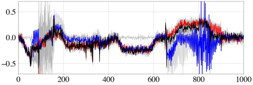
Autotuning HMC for nullspace exploration 945
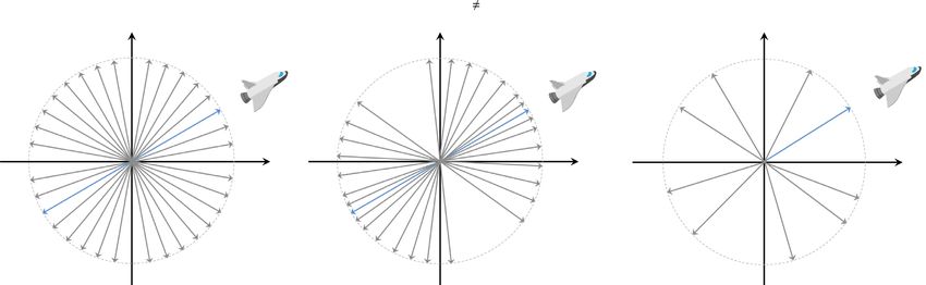
(a) (b) (c)
Downloaded from https://academic.oup.com/gji/article/227/2/941/6321848 by guest on 28 August 2021
Figure 2. 1-D harmonic oscillator. (a) Amplitude of an oscillator with circular frequency mtrue = 1. Randomly perturbed (noisy) amplitude observations are
shown as blue dots, and an estimated model with period m0 = 1.1 as grey curve. (b) A random collection of Hamiltonian trajectories drawn from the tolerance
distribution χ (ε|m0 ) = ρ(χ 0 + ε|m0 ) + kδ(ε) is shown in the top panel. Colour coding corresponds to the actual tolerance value ε, with larger values plotted
in more intense tones of red. The ith trajectory follows an iso-curve of the Hamiltonian H = U + K and samples misfit values below U(mi ) + ε i , as plotted in
identical colours in the lower panel. For better visibility, kinetic energies (misfits) of individual trajectories are slightly offset from the complete misfit curve,
shown as grey curve. The kinetic energy of the initial model m0 = 1.1 is indicated by a grey line. (c) Joint distribution ρ(p, m) = ρ(p|m)ρ(m) with exponential
colour scale. Models with low misfit, for instance around m = 1.0, admit larger tolerances, and vice versa.
that the elements of the observed data vector dobs, i = uobs (ti ) are 2.4.2 Exploring a high-dimensional Gaussian
independently polluted by noise with a standard normal distribution,
In the important class of linear inverse problems with normally
justifying the use of the root-mean-square misfit
distributed observational errors, the misfit χ (m) takes the form
Nd
1 T −1
χ (m) = [di (m) − dobs,i ]2 . (10) χ (m) = m C m, (11)
2
i=1
with some covariance matrix C (e.g. Parker 1994; Tarantola 2005;
For a fixed estimated frequency m0 , the Gaussian observation errors Menke 2012). While still being a simplistic case, it provides use-
cause the misfit distribution ρ(χ |m0 ) to be a non-central chi-square ful insight into the mechanics of Hamiltonian nullspace sampling,
distribution (Abramowitz & Stegun 1972) with an estimated non- especially when the eigenvalues of C differ by several orders of
centrality parameter λ ≈ max (χ 0 − Nd , 0) (e.g. Saxena & Alam magnitude.
1982). Therefore, a plausible distribution of the tolerance ε ex- Here, we consider a 1000-D model space and a diagonal co-
presses the probability of obtaining a misfit χ that exceeds χ 0 . As variance matrix with entries ranging linearly from C1, 1 = 0.01 to
shown in Appendix A1, this distribution is given by χ (ε|m0 ) = ρ(χ 0 C1000, 1000 = 1.0. Furthermore, to make the explicit link to HMC,
+ ε|m0 ) + kδ(ε), with a constant k. we draw directional tolerances p from an Nm -dimensional Gaussian
Successively drawing random √ tolerances εi from χ (ε|mi ) pro- with covariance M = I, meaning that the mass matrix M equals
vides initial momenta pi = ± 2Mε for Hamiltonian nullspace ex- the unit matrix. It follows that the generalized nullspace sampling
ploration. The sign can be chosen arbitrarily because momentum introduced in Section 2.3 produces samples of the joint distribution
space is symmetric in p. The same is true for the mass M, which is 1 Tp 1 T C−1 m
balanced against pi to always yield the same initial kinetic energy, ρ(p, m) ∝ e− 2 p e− 2 m . (12)
according to (6). In this example, we choose the plus sign and M =
1. Since Hamilton’s equations for this case cannot be solved ana- Fig. 3 summarizes the result after drawing 3000 samples, of which
lytically, we rely on a numerical approximation, which we compute the first 1000 are ignored as burn-in. As in the previous example,
using the leapfrog method (Appendix C). A collection of Hamil- we solve Hamilton’s equations using the leapfrog algorithm (Ap-
tonian trajectories for tolerances drawn from χ (ε|mi ) is shown in pendix C). While the approximated 1-D marginal of parameter m1
Fig. 2(b). Each trajectory traces an iso-line of the total energy H(p, in Fig. 3 a resembles the desired Gaussian with standard deviation
m), thereby reaching alternative models with misfit below χ i + εi . 0.1, the 1-D marginal of m1000 appears bimodal instead of Gaussian,
Following the sampling procedure described in Section 2.3 en- indicating that the number of samples is insufficient. The seemingly
sures that the trajectory end points sample the generalized nullspace different convergence speeds can be explained with the sample au-
distribution ρ(p, m), displayed in Fig. 2(c). As intuitively expected, tocorrelations of the two components,
smaller misfits (larger probabilities for some ε = const.) admit N
m l,i m l+k,i
larger tolerances, and vice versa. ci (k) = l=1N
, (13)
l=1 m l,i m l,i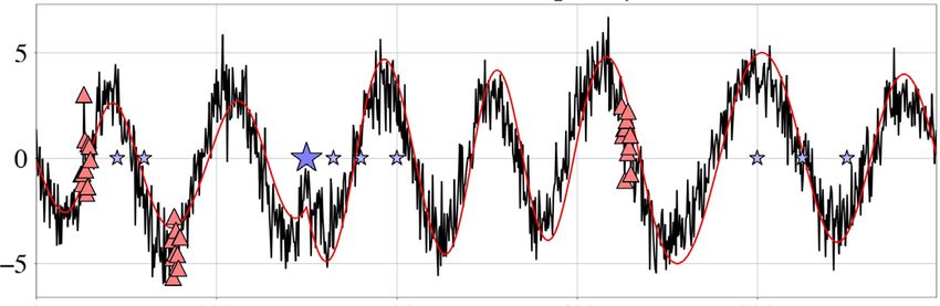
946       A. Fichtner et al.

    (a)                                (b)                                 (c)                                         (d)

Figure 3. Summary of HMC sampling of the 2×1000-D Gaussian in eq. (12). The model covariance matrix C is diagonal, with elements ranging linearly
from C1, 1 = 0.01 to C1000, 1000 = 1.0. The mass matrix M equals the unit matrix I. Of the 3000 samples used, 1000 are ignored as burn-in. (a,b) 1-D
marginals for parameters m1 and m1000 . (c) Autocorrelations averaged over 100 HMC runs of the sample chains for m1 and m1000 , with corresponding effective
sample fractions. (d) 2-D projection of a representative Hamiltonian trajectory (red, starting point in blue), with the target Gaussian shown in greyscale in the

                                                                                                                                                                    Downloaded from https://academic.oup.com/gji/article/227/2/941/6321848 by guest on 28 August 2021
background.

where N is the number of samples (excluding burn-in). The sam-                      0.15, meaning that one in around six samples is statistically inde-
ple autocorrelations in Fig. 3(c) reveal that the m1 -components of                 pendent. These properties are reflected in the 2-D projection of a
successive samples are practically uncorrelated. In contrast, the                   representative trajectory in Fig. 4(d), which makes similarly fast
m1000 -components are correlated over hundreds of samples, sug-                     progress in m1 - and m1000 -direction.
gesting that model space exploration in m1000 -direction is vastly
less efficient. In addition to being a qualitative measure of sample
dependence, the autocorrelation plays an important role in error                    2.5 Problem statements and outlook
estimates of Monte Carlo integration (e.g. Geyer 1992) and permits
estimates of the effective sample size (e.g. Ripley 1987; Krass et al.              In the previous sections, we introduced a framework for the ex-
1998; Gelman et al. 2013),                                                          plicit computation of alternative models with misfit below a defined
                                                                                    threshold, and the sampling of the generalized nullspace distribu-
                 N                                                                  tion ρ(p, m). While being conceptually straightforward, the main
Neff =          ∞             .                                       (14)
          1+2     k=1 ci (k)                                                        difficulty lies in the selection of tuning parameters that ensure the
                                                                                    efficient computation of models that are independent. These tuning
For uncorrelated√ samples, the Monte Carlo integration
                                                 √         error is pro-
                                                                                    parameters include the mass matrix M, the integration time step τ ,
portional to 1/ N , but only proportional to 1/ N eff , when samples
                                                                                    and the total length of the trajectory T . Each of these tuning param-
are correlated. Therefore, the effective sample fraction Neff /N serves
                                                                                    eters comes with its own subproblem, explained in the following
as an exchange rate that accounts for sample correlation. In prac-
                                                                                    paragraphs.
tice, the infinite sum in (14) must be approximated by a truncated
version, because the available number of samples is finite, and be-
cause ci (k) has a long noisy tail (Bartlett 1946). We follow (Gelman
et al. 2013) in terminating the summation when the sum of two suc-                  2.5.1 The mass matrix and local Hessian approximations
cessive autocorrelation values is zero for the first time. Applied to               Section 2.4.2 suggests that the mass matrix M should approximate
our example, we obtain effective sample fractions of 0.3286 for m1                  the local Hessian H(m) of χ (m). When χ (m) is quadratic, as in
and 0.0047 for m1000 , meaning that only one in around 1/0.0047 ≈                   eq. (11), we simply have H = C−1 . In the majority of applications,
213 samples is statistically independent in m1000 -direction. Though                however, H(m) is a priori unknown, and it can neither be computed
numerous other definitions and implementations of the effective                     nor stored explicitly. Furthermore, a factorization H = SST , needed
sample size have been proposed (e.g. Kong 1992; Martino et al.                      to draw samples of the directional tolerance p, as described in
2016), we will adhere to the version introduced above, as it can be                 Section 2.2, is usually unavailable.
easily computed and interpreted.                                                       We address the local approximation of the Hessian in Section 3
   The differences in effective sample fractions for m1 and m1000                   with the formulation of a factorized version of the L-BFGS method,
can be understood by examining a typical Hamiltonian trajectory,                    known from non-linear optimization (Nocedal 1980; Liu & Nocedal
shown in Fig. 3(d). In m1 -direction, the artificial particle makes                 1989; Nocedal & Wright 1999), and recently applied to geophysical
rapid progress, exploring different parts of model space. In con-                   inverse problems (e.g. Prieux et al. 2013; Métivier & Brossier 2016;
trast, progress in m1000 -direction is comparatively slow, meaning                  Modrak & Tromp 2016; Thrastarson et al. 2020; van Herwaarden
that all models along the trajectory have strongly correlated m1000 -               et al. 2020).
components.The trajectory in Fig. 3(d) also suggests a solution to
the problem of widely varying convergence speed, at least in the
case of the simple quadratic misfit (11). In fact, changing the mass
                                                                                    2.5.2 Integration length, Poincaré recurrence and energy drift
matrix from M = I to M = C−1 causes the trajectories to oscillate
equally fast in all directions (Fichtner et al. 2019). As a conse-                  To some extent, the strong correlation of successive samples, il-
quence, the 1-D marginals for m1 and m1000 , shown in Figs 4(a) and                 lustrated in Section 2.4.2, could be overcome by computing longer
(b), are both approximately Gaussian, with variances of around 0.01                 Hamiltonian trajectories, that is, by increasing the integration length
and 1.0, respectively. Furthermore, instead of being correlated over                T . However, in addition to being computationally expensive, this
hundreds of samples, both effective sample fractions are around                     approach is inherently limited by Poincaré recurrence (e.g. Poincaré
Autotuning HMC for nullspace exploration                 947

   (a)                               (b)                                (c)                                      (d)

Figure 4. Summary of HMC sampling with a setup identical to the one in Fig. 3, except for choosing the mass matrix M = C−1 . (a,b) 1-D marginals for
parameters m1 and m1000 . (c) Autocorrelations averaged over 100 HMC runs of the sample chains for m1 and m1000 , with corresponding effective sample
fractions. (d) 2-D projection of a representative Hamiltonian trajectory (red, starting point in blue), with the target Gaussian shown in greyscale in the

                                                                                                                                                             Downloaded from https://academic.oup.com/gji/article/227/2/941/6321848 by guest on 28 August 2021
background.

1890; Landau & Lifshitz 1976; Stephani & Kluge 1995). The ar-                   3 AU T O T U N I N G B Y L I M I T E D - M E M O RY
bitrarily close return of a trajectory to a previously visited point            Q UA S I - N E W T O N U P D AT I N G
after some sufficiently long time will introduce correlations that we
                                                                                For didactic reasons, we present the autotuning approach in sev-
actually wanted to avoid.
                                                                                eral small steps, starting with a condensed summary of the BFGS
   An equally profound complication is energy drift, that is, imper-
                                                                                method, and ending with a collection of measures that help to im-
fect energy conservation of numerical integrators for Hamilton’s
                                                                                prove convergence and stability of the method.
equations (e.g. Toxvaerd 1994; Toxvaerd et al. 2012). As shown in
Appendix C2, energy conservation of the leapfrog method, and of
the nearly identical Verlet integrator (Verlet 1967), is only correct
                                                                                3.1 BFGS updating of the mass matrix
to first order in the integration time step τ . Though this may be
improved with high-order integrators (Yoshida 1990; Martyna &                   In the context of non-linear optimization, the BFGS method (Broy-
Tuckerman 1995), exact energy conservation requires implicit in-                den 1970; Fletcher 1970; Goldfarb 1970; Shanno 1970; Nocedal &
tegration schemes (Simo et al. 1992; Quispel & McLaren 2008),                   Wright 1999) is used for the iterative approximation of the local
which are computationally out of scale for high-dimensional inverse             inverse Hessian H−1 , which then serves as a computationally less
problems.                                                                       expensive substitute of the exact Hessian in a Newton iteration. To
   In the context of generalized nullspace sampling, energy drift               summarize BFGS, we introduce the auxiliary vectors
has two main effects: (1) the misfit of models along a Hamil-
tonian trajectory may not actually be below the defined toler-                  sk = mk+1 − mk ,          yk = ∇U (mk+1 ) − ∇U (mk ),                (15)
ance and (2) the acceptance rate of the random sampling intro-                  where the subscript k denotes the sample index. Starting from a
duced in Section 2.3 may drop substantially because the accep-                  positive definite initial guess H−1
                                                                                                                 0 of the inverse Hessian of U, the
tance criterion involves the ratio between the initial and the final            BFGS iteration computes successive approximations of H−1 as
Hamiltonian.                                                                                          −1
   In the context of standard HMC, where the directional toler-                 H−1
                                                                                  k+1 = I − ρk sk yk Hk
                                                                                                    T
                                                                                                             I − ρk yk skT + ρk sk skT ,      (16)
ance distribution is Gaussian, the integration length T has received
                                                                                with the scaling factor
considerable attention (e.g. Mackenzie 1989; Hoffmann & Gelman
2014). Based on the local Hessian approximation, we present in                           1
                                                                                ρk =          .                                                      (17)
Section 3.4.2 a semi-analytical argument for the suitable choice of                    ykT sk
the integration length, which empirically works well in numerical
                                                                                The latter must be strictly positive to ensure that successive up-
experiments.
                                                                                dates are positive definite. The corresponding Hk+1 easily follows
                                                                                from the Sherman–Morrison formula (Bartlett 1951; Nocedal &
                                                                                Wright 1999). Assuming that Hk+1 approximates the local Hessian
                                                                                H(mk+1 ), we may use Hk+1 as mass matrix to draw the subse-
                                                                                quent sample mk+1 . This approach raises two issues: (1) Generat-
                                                                                ing random momenta, or directional tolerances p, as described in
2.5.3 Numerical stability and adaptive time stepping                            Sections 2.2 and 2.3, requires a factorization of the mass matrix,
                                                                                M = SST , for instance, a Cholesky decomposition. However, the
The numerical stability of leapfrog, and of any other explicit inte-
                                                                                number of operations needed to compute S is of order Nm3 , meaning
grator, depends on the eigenvalues of the mass matrix M (see, for
                                                                                that it is out of scale for many relevant applications. (2) The matrices
instance, Appendix C1). Hence, as M changes during the gen-
                                                                                H−1
                                                                                  k may be too large to be stored.
eralized nullspace sampling, the integrator may become unsta-
ble. To prevent such instability, we propose in Section 3.4.3 an
adaptive time stepping scheme, where the integration time step
                                                                                3.2 Factorized BFGS updating (F-BFGS)
can be adjusted. It rests entirely on estimates of energy con-
servation, thereby avoiding the need to compute eigenvalues of                  To produce a scalable algorithm, we aim to compute the matrix
M.                                                                              factor S directly, using a modified BFGS update equation. Following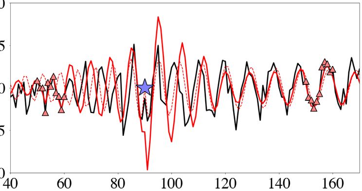
948         A. Fichtner et al.

an approach indicated by Broodlie et al. (1973), we first write the       3.3 Limited-memory factorized BFGS updating
regular BFGS update from eq. (16) in the factorized form                  (LF-BFGS)
                  −1            T
H−1
  k+1 = I + uk vk Hk
                T
                         I + uk vkT ,                          (18)       The factorized updating formulae (28) straightforwardly enable a
                                                                          limited-memory approach, similar to the standard limited-memory
with two vectors uk and vk that remain to be determined. First, we
                                                                          BFGS concept of Nocedal (1980) and Liu & Nocedal (1989). In
note that eq. (16) may be expanded to
                                                                          fact, letting h be some arbitrary vector, we may write
H−1     −1
 k+1 = Hk + ak ak − bk ak − ak bk ,
                T       T       T
                                                                  (19)
                                                                                              vk ukT
                                                                          Sk+1 h = I −
where we defined the auxiliary variables                                                   1 + vkT uk

γk2 = ρk2 ykT H−1
               k yk + ρk ,                                       (20a)                                 T
                                                                                                 vk−1 uk−1               v0 u0T
                                                                                     × I−                    ... I −              S0 h. (29)
                                                                                               1 + vk−1 uk−1
                                                                                                     T
                                                                                                                       1 + v0T u0
ak = γk sk ,                                                     (20b)
                                                                          Typically, the initial matrix S0 equal the unit matrix I. Defining
     ρk                                                                   h0 = S0 h, eq. (29) takes the form of a sequential update,
bk = H−1    yk .                                          (20c)
     γk k
                                                                                           vi uiT                    uiT hi
                                                                          hi+1 = I −                 hi = hi − vi             , i = 0, ..., k,

                                                                                                                                                      Downloaded from https://academic.oup.com/gji/article/227/2/941/6321848 by guest on 28 August 2021
Comparing the expanded form of (18) and (19), motivates the fol-
                                                                                        1 + vi ui
                                                                                                T
                                                                                                                   1 + viT ui
lowing ansatz for the vectors uk and vk ,
                                                                                                                                            (30)
uk = ak ,                                                        (21a)
                                                                          which eventually gives
vk = −Hk (bk + θ ak ),                                           (21b)    Sk+1 h = hk+1 .                                                     (31)
with some scalar θ . To find θ , we substitute eqs (21a) and (21b) into   Most importantly, eq. (30) only contains vector–vector products,
eq. (18),                                                                 eliminating the need to explicitly compute and store any matri-

H−1       −1
  k+1 = Hk + ak ak (bk + θ ak ) Hk (bk + θ ak ) − 2θ
                     T              T
                                                                          ces. Furthermore, the sequence can be limited to the last + 1
            − bk akT − ak bkT .                                   (22)    vector pairs (uk , vk ), ..., (uk− , vk− ), which further reduces storage
                                                                          requirements at the expense of a more incorrect but hopefully still
The comparison of eq. (22) to eq. (19) shows that θ must satisfy the      acceptable Hessian approximation (Nocedal & Wright 1999). Fol-
quadratic equation                                                        lowing this approach, similar equations can be found for products
(bk + θ ak )T Hk (bk + θ ak ) − 2θ = 1,                           (23)    of h with the inverse and transpose of Sk+1 .

or, slightly reordered,
 T                                                                  3.4 Further measures to improve convergence and stability
 ak Hk ak θ 2 + 2 akT Hk bk − 1 θ + bkT Hk bk − 1 = 0.            (24)
To express the polynomial coefficients in eq. (24) in terms of sk and     3.4.1 Iterative updating of the initial matrix
yk , we re-substitute eqs (20a) and (20b), which leads to
                                                                          Despite being, for simplicity, presented as a constant in Section 3.3,
 2 T               ρk
 γk sk Hk sk θ 2 = 2 .                                           (25)     the initial matrix factor S0 can and should be updated to improve
                     γk                                                   convergence. A constant S0 implies that the LF-BFGS algorithm
Eq. (25) yields two real-valued solutions for θ provided that ρ k >       has a memory of samples, which may be small compared to the
0, which is identical to the condition needed to ensure positive-         model space dimension Nm . Updating S0 may increase the memory,
definite BFGS updates (e.g. Nocedal & Wright 1999). The previous          meaning that more than samples effectively contribute to the
set of equations provides a simple recipe for the factorized BFGS         Hessian approximation.
(F-BFGS) updating of H−1 k based on the computation of the vectors
                                                                             Most straightforwardly, S0 is replaced in regular intervals, typi-
uk and vk through eqs (20) and (21). A factorized update of Hk now        cally every samples, by the square root of the diagonal elements
follows directly from the inversion of eq. (18),                          of the current Hessian approximation, that is,
                  −1              −1
Hk+1 = I + vk ukT      Hk I + uk vkT     ,                     (26)         diag Hk → S0 .                                                    (32)
combined with the Shermann–Morrison formula for the inverse of            We note that any updating of S0 requires a recalculation of the vector
rank-one updates (Bartlett 1951; Nocedal & Wright 1999)                   sequences u0 , u1 , ... and v0 , v1 , ..., as they depend on S0 .
                −1           vk ukT
    I + vk ukT         =I−              .                         (27)
                             1 + vkT uk                                   3.4.2 Integration length
Assuming that a factorization Hk = Sk SkT is available from previous      The choice of a suitable integration length T is a balancing act
F-BFGS iterations, eqs (26) and (27) imply that the updated matrix        between a large T that ensures rapid model space exploration and
factor Sk+1 and its inverse S−1
                             k+1 are given by                             a small T to limit computational cost. Fortunately, using the LF-
                                                                         BFGS Hessian Hk as mass matrix provides some useful guidance.
                vk ukT
Sk+1 = I −                 Sk ,     S−1
                                      k+1 = Sk
                                              −1
                                                  I + vk ukT .  (28)      In fact, as Hk , and therefore M, approach the true Hessian H,
              1 + vkT uk
                                                                          the Hamiltonian trajectories converge towards segments of Nm -
Knowing the matrix factors Sk+1 and S−1k+1 , allows us to compute all     dimensional circles with circular frequency 2π . Hence, in the case
(inverse) Hessian-vector products and to generate random momenta          of a roughly constant Hessian, we observe approximate Poincaré
from a Gaussian with covariance M = Hk . We parenthetically re-           recurrence for T = 2π , and about half the trajectory has been tra-
mark that Sk is usually dense and not a Cholesky factor of Hk .           versed for T = π .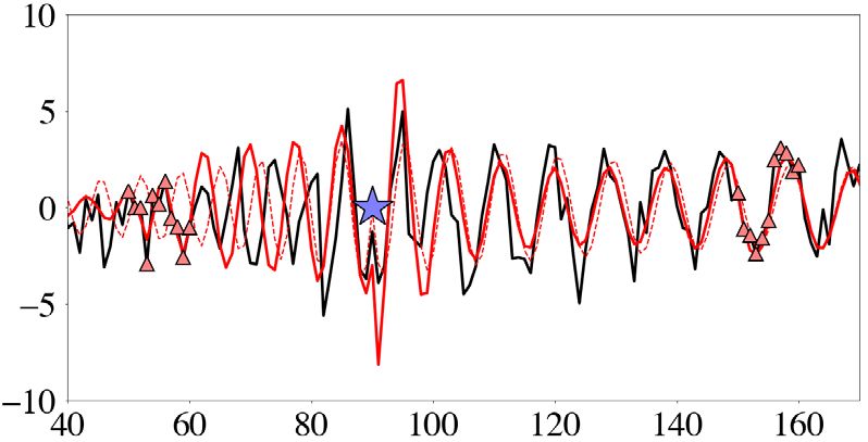
Autotuning HMC for nullspace exploration              949

   When the Hessian is not approximately constant, the above argu-          In the following section, we introduce two variations of the au-
ment looses precision. Nevertheless, setting T ≈ π with some ran-        totuning approach that preserve the Markov property, possibly at
dom variations to avoid cyclic behaviour of the sampler (Mackenzie       the expense of reduced efficiency (depending on the specifics of an
1989) is an empirically useful choice that we adopted in all of the      application).
following examples.

                                                                         3.6 Variations of the theme
3.4.3 Initial and adaptive time stepping
                                                                         The set of algorithms presented in Sections 3.1–3.4 provides a
The (leapfrog) integration time step τ is controlled by the need        general autotuning framework. As suggested by the No-Free-Lunch
to (1) conserve energy of the nullspace shuttle, (2) maintain high       theorem (e.g. Wolpert & Macready 1997; Mosegaard 2012), its
acceptance rates of the nullspace sampler and (3) ensure numerical       efficiency may be increased through slight adaptations that account
stability. As demonstrated in Appendix C1, numerical stability re-       for prior knowledge. Two possible adaptations that we will revisit in
quires τ ≤ 2/ λmax (M−1 H), where λmax (M−1 H) is the maximum           later numerical examples are presented in the following paragraphs.
eigenvalue of the matrix product M−1 H.
   An initial estimate of a conservative τ may be obtained by

                                                                                                                                                 Downloaded from https://academic.oup.com/gji/article/227/2/941/6321848 by guest on 28 August 2021
simple trial-and-error, that is, the testing of candidate time steps
                                                                         3.6.1 Diagonal freezing
until integration is stable. Alternatively, one may have estimates of
the maximum eigenvalue of the Hessian near the estimated model,          In cases where the Hessian is a priori known to be roughly diagonal
λmax [H(m0 )], from physical arguments or the application of second-     and roughly invariant, the generalized nullspace sampling may be
order adjoint methods (e.g. Santosa & Symes 1988; Pratt et al.           accelerated by estimating the diagonal of the Hessian using few
1998; Fichtner & Trampert 2011). Setting the initial mass matrix to      very short sample chains starting from different initial models. The
λmax [H(m0 )] I then causes the maximum allowable τ to be around        resulting approximation of the Hessian diagonal is then used as a
2, meaning that τ ≈ 1 is likely to be a useful and conservative         constant mass matrix in a sample chain that is sufficiently long to
starting point.                                                          ensure convergence.
   Successive updating of the mass matrix with the LF-BFGS Hes-             The freezing of the diagonal after its initial estimation has the
sian affects numerical stability because the maximum eigenvalue of       advantage of avoiding both the computational cost of on-the-fly au-
M−1 H changes. Since repeated eigenvalue estimations are compu-          totuning and the potential bias introduced by an otherwise inexact
tationally out of scale, an alternative approach for the adjustment      Markov chain (see Section 3.5). These advantages have to be bal-
of τ is needed. For this, we may exploit the otherwise undesirable      anced on a case-by-case basis against the disadvantage of ignoring
fact that energy conservation of the leapfrog scheme is only correct     off-diagonal elements and a non-constant Hessian. An example of
to first order in τ , as shown in Appendix C2. The deterioration of     the diagonal freezing approach is presented in Section 4.2.
energy conservation may therefore be used as a proxy for upcoming
numerical instability.
   In practice, the adaptation of τ is most easily implemented by       3.6.2 Macroscopic autotuning
monitoring the acceptance rate R averaged over roughly samples.
The decrease of R below some threshold Rmin relates directly to          When the generalized nullspace has fine-scale structure, for in-
decreasing energy conservation, suggesting that τ should be re-         stance, in the form of numerous local minima, superimposed on
duced to a smaller value γ τ with γ < 1. Conversely, when R             some broad-scale background that is roughly Gaussian, we may
is above some threshold Rmax , the time step may be increased to         borrow basic ideas from tempering (e.g. Kirkpatrick et al. 1983;
τ /γ to reduce computational costs. In the following examples, we       Marinari & Parisi 1992; Geyer & Thompson 1995; Sambridge
use Rmin = 0.65, Rmax = 0.85 and γ = 0.80, as empirically useful         2014). Instead of considering the original generalized nullspace
values.                                                                  distribution,
                                                                                                          1 T M−1 p
                                                                         ρ(p, m) = e−H (p,m) = e−U (m) e− 2 p         ,                  (33)
3.5 Loss of the Markov property                                          we consider a tempered version,
The sequence of generalized nullspace samples produced by the                                                       − 12 pT M−1
autotuning algorithm is not an exact Markov chain where the next         ρ 1/T (p, m) = e−H (p,m)/T = e−U (m)/T e            T p
                                                                                                                                   ,     (34)
model only depends on the current one. In fact, the next model           with a temperature T > 1 and a tempered or macroscopic mass
depends on the current mass matrix, which is controlled by >             matrix
1 previous misfit and gradient evaluations. Hence, the stochastic
                                                                                 1 −1
sampling process is not memoryless, as required by the detailed          M−1
                                                                          T =      M .                                                   (35)
balance proof in Appendix B. Similar to other approximate Markov                 T
chain methods (e.g. Bardenet et al. 2014; Fox & Nicholls 1997;           By design, tempering suppresses detail while enhancing and broad-
Korattikara et al. 2014; Scott et al. 2016), the autotuning algorithm    ening macroscopic features of the distribution, as schematically
may effectively sample a different distribution, thereby introducing     illustrated in Fig. 5. The macroscopic shape of the generalized
bias.                                                                    nullspace may be captured using an LF-BFGS approximation of
   In realistic applications, where the nullspace distribution ρ(p, m)   the macroscopic Hessian, again using a small number of very
is unknown from the outset, the bias may be difficult to estimate.       short chains starting from different initial models. Subsequently,
Nevertheless, the autotuning algorithm may still produce indepen-        the macroscopic Hessian in LF-BFGS representation can be scaled
dent nullspace samples more efficiently than a Hamiltonian sampler       back to a hopefully useful and constant mass matrix of the actual
with unit mass matrix.                                                   problem using eq. (35).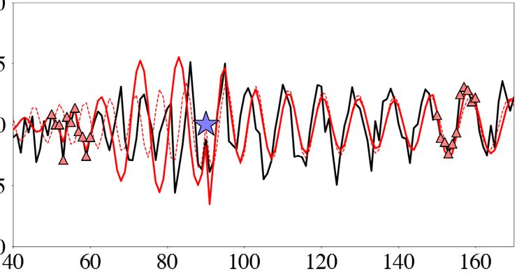
950      A. Fichtner et al.

  (a)                                                                       (b)

Figure 5. Schematic illustration of the effect of tempering, which transforms the multimodal distribution in (a) into the smoother, more Gaussian-like
distribution in (b).

  The advantages and drawbacks of macroscopic autotuning are                      4.2 Modified Styblinski–Tang function
similar to those of diagonal freezing in Section 3.6.1. Further-
                                                                                  Originally developed for the benchmarking of global optimiza-
more, by virtue of eq. (34), macroscopic autotuning is limited

                                                                                                                                                                 Downloaded from https://academic.oup.com/gji/article/227/2/941/6321848 by guest on 28 August 2021
                                                                                  tion algorithms in the context of neural network design, the Nm -
to cases where the tolerance distribution is Gaussian. An ex-
                                                                                  dimensional Styblinski–Tang function (Styblinski & Tang 1990)
ample of the macroscopic autotuning approach can be found in
                                                                                  is non-convex and multimodal, with 2 Nm local minima. Since the
Section 4.3.
                                                                                  Styblinski–Tang function can take negative values, we use a mod-
                                                                                  ified version, described in Appendix D1, in order to define a mis-
                                                                                  fit χ (m). Furthermore, we introduce interparameter trade-offs. To
                                                                                  again make the connection to HMC, we use an Nm -dimensional
4 P E R F O R M A N C E A N A LY S I S U S I N G
                                                                                  Gaussian for the proposal of directional tolerances p. In this exam-
A N A LY T I C A L T E S T F U N C T I O N S
                                                                                  ple, we again choose Nm = 1000.
The following paragraphs are dedicated to a performance analysis                      As a reference, we consider a chain of 1 million samples com-
of the autotuning approach proposed in Section 3. The focus will                  puted with constant unit mass matrix, M = I, and constant time
be on the two main goals of this work: (1) the efficient computation              step, τ . By laborious trial and error, we determined τ and the
of independent alternative models and (2) the efficient sampling of               integration length T such that the effective sample fraction of the
the nullspace distribution ρ(p, m). While the former can be easily                least constrained parameter, m1000 in this case, is maximized. Specif-
quantified in terms of the effective sample size, defined in (14), the            ically, we found τ = 0.35 and T = 2.45 to produce a maximum
latter is more difficult because there is no universally valid quantifier         effective sample fraction of 1.1 × 10⁻⁴ , as illustrated in Fig. 7(a).
of Markov chain convergence, though numerous proxies have been                    Small changes of τ and T may increase the effective sample frac-
proposed (e.g. Gelman & Rubin 1992; Geweke 1992; Raftery &                        tion slightly, but order-of-magnitude improvements are unlikely to
Lewis 1992; Cowles & Carlin 1996; Roy 2019).                                      be possible. The small value of the effective sample fraction mostly
   To quantify convergence, we conduct the performance anal-                      reflects the number of samples required to switch between different
ysis using analytical test functions for which lower-dimensional                  modes of the modified Styblinski–Tang function. This is in contrast
marginals and moments of various orders can be computed exactly.                  to the Gaussian, where the effective sample fraction describes the
Unavoidably, this widely-used approach to performance analysis is                 (in-)dependence of samples within the only existing mode.
limited by the small number of test functions that we can consider.                   Using the diagonal freezing variant of autotuning from Sec-
Nevertheless, it provides indications about the circumstances under               tion 3.6.1, we then compute a constant diagonal mass matrix by
which the proposed algorithms are useful.                                         averaging the diagonals of LF-BFGS Hessian approximations ob-
   In all of the following examples, including those in Section 5,                tained from 10 sample chains. Each of these chains starts from a
we use on average five leapfrog integration steps, meaning that the               different, randomly selected initial model and only contains 200
number of misfit and gradient evaluations is around five times larger             samples. The resulting effective sample fraction is 5.5 × 10⁻⁴ , that
than the number of samples.                                                       is, 5 times larger than in the most optimal case with unit mass matrix.
                                                                                  Hence, the sampler manages to switch into a different mode of the
                                                                                  distribution about every 2000 samples, instead of 10 000 samples
                                                                                  in the case without autotuning. The differences in effective sample
4.1 Return to the high-dimensional Gaussian                                       fractions translate to differences in convergence. Since statistical
                                                                                  moments are either hard to interpret for a multimodal distribution
Starting with the simplest possible case, we return to the sampling of            (e.g. means and variances) or highly susceptible to outliers (higher
the 1000-D Gaussian, previously presented as motivating example                   moments such as skewness or kurtosis), we consider convergence
in Section 2.4.2. Updating the initial mass matrix M = I with the au-             to the exact 2-D marginal of m1 and m1000 , which we can compute
totuning procedure described in Section 3, reproduces Fig. 4 almost               semi-analytically. For this, we measure the discrepancy between the
exactly. Hence, we achieve effective sample sizes as if we had used               exact marginal ρ(m1 , m1000 ) and the sample-approximated marginal
M = H = C−1 from the outset. The time-step adaptivity guided by                   ρ̃(m 1 , m 1000 ) in terms of the Kullback–Leibler divergence or rela-
the average acceptance rate ensures that the leapfrog integration                 tive information content (e.g. Shannon 1948; Kullback & Leibler
remains numerically stable. This is summarized in Fig. 6. Since the               1951; Tarantola & Valette 1982; Tarantola 2005),
target distribution is Gaussian, the LF-BFGS approximation to the
Hessian eventually becomes stationary in this example, meaning
that the initially approximate Markov chain converges towards an
                                                                                                                       ρ̃(m 1 , m 1000 )
exact Markov chain.                                                               DK L =     ρ̃(m 1 , m 1000 ) log10                     dm 1 dm 1000 .   (36)
                                                                                                                       ρ(m 1 , m 1000 )
Autotuning HMC for nullspace exploration 951
(a) (b)
Figure 6. Time-step adaptivity during autotuning of the nullspace sampler. (a) Acceptance rate R averaged over the previous 20 samples. (b) Variable integration
time step τ that aims to keep R between the threshold values Rmax = 0.85 and Rmin = 0.5.
Downloaded from https://academic.oup.com/gji/article/227/2/941/6321848 by guest on 28 August 2021
(a) (b)
Figure 7. Autocorrelations of the most constrained parameter, m1 , and the least constrained parameter, m1000 , of the modified Styblinski–Tang function,
averaged over 10 realizations of sample chains with 1 million samples each. (a) Without autotuning, autocorrelation lengths are on the order of 10 000, meaning
that around 10 000 samples are needed to switch between modes of the modified Styblinski–Tang function (eq. (D2)). The corresponding effective sample
fractions, N/Neff , are on the order of 1 × 10⁻⁴ . (b) Autocorrelations and effective sample fractions when the diagonal freezing variant of autotuning is used.
The effective sample fractions increased by a factor of about 5.
In this context, DKL can be interpreted as a loss of information (in in Fig. D2. For the model space dimension, we again choose Nm =
digits) that results from an inaccurate approximation of the exact 1000.
distribution. As illustrated in Fig. 8, the autotuning variant of the To establish a reference, we disable autotuning and repeat the
sampler approximates the exact marginal with order of magnitude trial-and-error search over the integration time step, τ , and
10 000 samples, assuming DKL = 0.1 as a reasonable threshold. the integration length, T , with the aim to maximize the effec-
Around five times more samples are needed without autotuning. We tive sample fraction of the least constrained parameter, m1000 .
note that other measures of convergence are, of course, possible, but Nearly optimal values for chains with 1 million samples are τ
unlikely to change the general conclusion, given that the effect of = 0.02 and T = 1.4, leading to low effective sample fractions
autotuning is not small. of 7.0 × 10⁻⁶ for m1 and 7.1 × 10⁻⁶ for m1000 . The corre-
sponding autocorrelation graphs are shown in Fig. 9(a). As for
the modified Styblinski–Tang function, the effective sample frac-
tions mostly reflect the average number of samples needed for the
4.3 Modified Rastrigin function transition between different modes of the multimodal probability
density.
Similar to the Styblinski–Tang function, the 2-D version of the
To improve convergence, we use the macroscopic autotuning
Rastrigin function was initially proposed as a performance test
approach presented in Section 3.6.2, using the temperature T =
function for optimization algorithms (Rastrigin 1974). Its higher-
100 and only 500 samples. The resulting LF-BFGS representation
dimensional generalization, proposed by Rudolph (1990), is given
of the mass matrix MT is then rescaled and kept constant during
by eq. (D5) in Appendix D2. Being highly oscillatory, the Rastrigin
the subsequent sampling of the modified Rastrigin function. The
function is non-convex and equipped with an infinite number of lo-
resulting autocorrelation graphs are shown in Fig. 9(b). Relative to
cal maxima. Since the Rastrigin function is positive semi-definite, it
the previous chain without autotuning, effective sample fractions
can be used directly as a misfit function. Yet, to mimic geophysical
increase by a factor of around 50, to 3.6 × 10⁻⁴ for m1 and 3.0 ×
inverse problems more closely, we introduce inter-parameter cor-
10−4 for m1000 .
relations and variable parameter sensitivities, as we previously did
The large differences of effective sample fractions translate to
for the Styblinski–Tang function. The resulting modified Rastrigin
differences in convergence towards the posterior distribution. As an
function is defined through eq. (D6), and some illustrations of the
example, we again consider the Kullback–Leibler divergence of the
function itself and its associated probability density are presentedYou can also read