Deep learning in bioinformatics: introduction, application, and perspective in big data era - bioRxiv
←
→
Page content transcription
If your browser does not render page correctly, please read the page content below
bioRxiv preprint first posted online Feb. 28, 2019; doi: http://dx.doi.org/10.1101/563601. The copyright holder for this preprint
 (which was not peer-reviewed) is the author/funder, who has granted bioRxiv a license to display the preprint in perpetuity.
                                    All rights reserved. No reuse allowed without permission.

                        Deep learning in bioinformatics: introduction,
                         application, and perspective in big data era

                           Yu Li             Chao Huang                  Lizhong Ding                 Zhongxiao Li
                          KAUST                 NICT                         IIAI                       KAUST
                          CBRC                  CAS                                                      CBRC
                          CEMSE                                                                         CEMSE

                                            Yijie Pan                                   Xin Gao ∗
                                             NICT                                       KAUST
                                              CAS                                        CBRC
                                                                                        CEMSE

                                                                 Abstract

                          Deep learning, which is especially formidable in handling big data, has achieved
                          great success in various fields, including bioinformatics. With the advances of
                          the big data era in biology, it is foreseeable that deep learning will become in-
                          creasingly important in the field and will be incorporated in vast majorities of
                          analysis pipelines. In this review, we provide both the exoteric introduction of
                          deep learning, and concrete examples and implementations of its representative
                          applications in bioinformatics. We start from the recent achievements of deep
                          learning in the bioinformatics field, pointing out the problems which are suitable to
                          use deep learning. After that, we introduce deep learning in an easy-to-understand
                          fashion, from shallow neural networks to legendary convolutional neural networks,
                          legendary recurrent neural networks, graph neural networks, generative adversarial
                          networks, variational autoencoder, and the most recent state-of-the-art architec-
                          tures. After that, we provide eight examples, covering five bioinformatics research
                          directions and all the four kinds of data type, with the implementation written in
                          Tensorflow and Keras. Finally, we discuss the common issues, such as overfitting
                          and interpretability, that users will encounter when adopting deep learning methods
                          and provide corresponding suggestions. The implementations are freely available
                          at https://github.com/lykaust15/Deep_learning_examples.

             1 Introduction
             With the significant improvement of computational power and the advancement of big data, deep
             learning has become one of the most successful machine learning algorithms in recent years [77]. It
             has been continuously refreshing the state-of-the-art performance of many machine learning tasks
             [72, 152, 60, 151] and facilitating the development of numerous disciplines [10, 149, 42, 91]. For
             example, in the computer vision field, methods based on convolutional neural networks have already
             dominated its three major directions, including image recognition [72, 52, 60], object detection
             [126, 125], and image inpainting [178, 186] and super-resolution [188, 78]. In the natural language
             processing field, methods based on recurrent neural networks usually represent the state-of-the-art
             performance in a broad range of tasks, from text classification [197], to speech recognition [55] and
             machine translation [151]. Researchers in the high energy physics field have also been using deep
                 ∗
                     All correspondence should be addressed to Xin Gao (xin.gao@kaust.edu.sa).

             Preprint. Work in progress.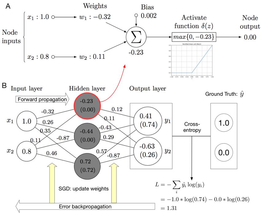
bioRxiv preprint first posted online Feb. 28, 2019; doi: http://dx.doi.org/10.1101/563601. The copyright holder for this preprint
 (which was not peer-reviewed) is the author/funder, who has granted bioRxiv a license to display the preprint in perpetuity.
                                    All rights reserved. No reuse allowed without permission.

                                                       Table 1: Abbreviations.
               Abbreviations       Full words                                            Reference
               AUC                 Area under curve                                      [171]
               CNN                 Convolutional neural networks                         [72]
               Cryo-EM             Cryogenic electron microscopy                         [102]
               Cryo-ET             Cryogenic electron tomography                         [50]
               CT                  Computed tomography                                   [76]
               DenseNet            Densely connected convolutional networks              [60]
               DNN                 Deep fully connected neural networks                  [77]
               DPN                 Dual path networks                                    [16]
               DR                  Dimensionality reduction                              [129]
               EEG                 Electroencephalogram                                  [149]
               GAN                 Generative adversarial networks                       [43]
               GCN                 Graph convolutional neural networks                   [69]
               RNN                 Recurrent neural networks                             [103]
               ResNet              Residual networks                                     [52]
               LSTM                Long short-term memory                                [44]
               MRI                 Magnetic resonance imaging                            [133]
               PET                 Positron emission tomography                          [84]
               PseAAC              Pseudo amino acid composition                         [20]
               PSSM                Position specific scoring matrix                      [85]
               ReLU                Rectified linear unit                                 [108]
               SENet               Squeeze-and-excitation networks                       [58]
               SGD                 Stochastic gradient descent                           [196]
               VAE                 Variational auto-encoder                              [30]

             learning to promote the search of exotic particles [10]. In psychology, deep learning has been used to
             facilitate Electroencephalogram (EEG) (the abbreviations used in this paper are summarized in Table
             1) data processing [149]. Considering its application in material design [97] and quantum chemistry
             [135], people also believe deep learning will become a valuable tool in computational chemistry [42].
             Within the computational physics field, deep learning has been shown to be able to accelerate flash
             calculation [91].
             Meanwhile, deep learning has clearly demonstrated its power in promoting the bioinformatics field
             [104, 5, 18], including sequence analysis [198, 3, 25, 156, 87, 6, 80, 169, 157, 158, 175], structure
             prediction and reconstruction [167, 90, 38, 168, 180, 196, 170], biomolecular property and function
             prediction [85, 204, 75, 4], biomedical image processing and diagnosis [35, 66, 41, 22, 160], and
             biomolecule interaction prediction and systems biology [95, 201, 203, 144, 145, 67, 165, 191].
             Specifically, regarding sequence analysis, people have used deep learning to predict the effect of
             noncoding sequence variants [198, 166], model the transcription factor binding affinity landscape [25,
             3, 166], improve DNA sequencing [87, 154] and peptide sequencing [156], analyze DNA sequence
             modification [143], and model various post-transcription regulation events, such as alternative
             polyadenylation [81], alternative splicing [80], transcription starting site [159, 157], noncoding RNA
             [181, 7] and transcript boundaries [139]. In terms of structure prediction, [167, 54] use deep learning
             to predict the protein secondary structure; [38, 196] adopt deep learning to model the protein structure
             when it interacts with other molecules; [170, 180, 168] utilize deep neural networks to predict protein
             contact maps and the structure of membrane proteins; [90] accelerates the fluorescence microscopy
             super-resolution by combining deep learning with Bayesian inference. Regarding the biomolecular
             property and function prediction, [85] predicts enzyme detailed function by predicting the Enzyme
             Commission number (EC numbers) using deep learning; [75] deploys deep learning to predict
             the protein Gene Ontology (GO); [4] predicts the protein subcellular location with deep learning.
             There are also a number of breakthroughs in using deep learning to perform biomedical image
             processing and biomedical diagnosis. For example, [35] proposes a method based on deep neural
             networks, which can reach dermatologist-level performance in classifying skin cancer; [66] uses
             transfer learning to solve the data-hungry problem to promote the automatic medical diagnosis; [22]
             proposes a deep learning method to automatically predict fluorescent labels from transmitted-light
             images of unlabeled biological samples; [41, 160] also propose deep learning methods to analyze

                                                                       2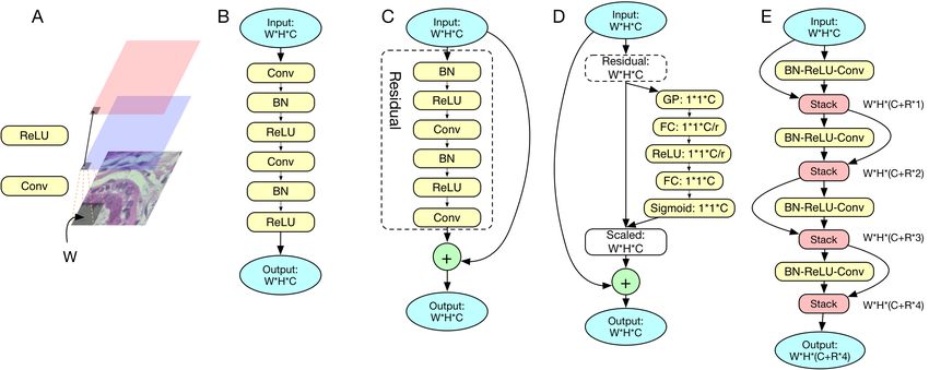
bioRxiv preprint first posted online Feb. 28, 2019; doi: http://dx.doi.org/10.1101/563601. The copyright holder for this preprint
 (which was not peer-reviewed) is the author/funder, who has granted bioRxiv a license to display the preprint in perpetuity.
                                    All rights reserved. No reuse allowed without permission.

                                Table 2: The applications of deep learning in bioinformatics.
               Research direction     Data                                   Data types Candidate                            References
                                                                                           models
               Sequence analysis      Sequence data (DNA sequence, 1D data                 CNN, RNN               [198, 3, 25,
                                      RNA sequence, et al.)                                                       156, 87, 6, 80,
                                                                                                                  157, 158, 175,
                                                                                                                  169]
               Structure prediction        MRI images, Cryo-EM images, flu- 2D data                     CNN, GAN, [167, 90, 38,
               and reconstruction          orescence microscopy images, pro-                            VAE       168, 180, 196,
                                           tein contact map                                                       170]
               Biomolecular prop-          Sequencing data, PSSM, structure 1D data,                    DNN, CNN, [85, 204, 75,
               erty and function           properties, microarray gene expres- 2D data,                 RNN       4]
               prediction                  sion                                structured
                                                                               data
               Biomedical image            CT images, PET images, MRI im- 2D data                        CNN, GAN            [35, 66, 41,
               processing      and         ages                                                                              22, 160]
               diagnosis
               Biomolecule interac-        Microarray gene expression, PPI, 1D data,                     CNN, GCN           [95, 201, 203,
               tion prediction and         gene-disease interaction, disease- 2D data,                                      165, 71, 191,
               systems biology             disease similarity network, disease- structured                                  67, 88]
                                           variant network                      data,
                                                                                graph data

             the cell imagining data. As for the final main direction, i.e., biomolecule interaction prediction and
             systems biology, [95] uses deep learning to model the hierarchical structure and the function of
             the whole cell; [203, 165] adopt deep learning to predict novel drug-target interaction; [201] takes
             advantage of multi-modal graph convolutional networks to model polypharmacy sides effects.
             In addition to the increasing computational capacity and the improved algorithms [61, 148, 52, 60,
             86, 146], the core reason for deep learning’s success in bioinformatics is the data. The enormous
             amount of data being generated in the biological field, which was once thought to be a big challenge
             [99], actually makes deep learning very suitable for biological analysis. In particular, deep learning
             has shown its superiority in dealing with the following biological data types. Firstly, deep learning
             has been successful in handling sequence data, such as DNA sequences [198, 166, 143], RNA
             sequences [110, 181, 7], protein sequences [85, 75, 4, 156], and Nanopore signal [87]. Trained
             with backpropagation and stochastic gradient descent, deep learning is expert in detecting and
             identifying the known and previously unknown motifs, patterns and domains hidden in the sequence
             data [140, 25, 3, 85]. Recurrent neural networks and convolutional neural networks with 1D filters
             are suitable for dealing with this kind of data. However, since it is not easy to explain and visualize
             the pattern discovered by recurrent neural networks, convolutional neural networks are usually the
             best choice for biological sequence data if one wants to figure out the hidden patterns discovered
             by the neural network [140, 3]. Secondly, deep learning is especially powerful in processing 2D
             and tensor-like data, such as biomedical images [90, 35, 22, 41, 160] and gene expression profiles
             [172, 14]. The standard convolutional neural networks [72] and their variants, such as residual
             networks [53], densely connected networks [60], and dual path networks [16], have shown impressive
             performance in dealing with biomedical data [22, 41]. With the help of convolutional layers and
             pooling layers, these networks can systematically examine the patterns hidden in the original map
             in different scales and map the original input to an automatically determined hidden space, where
             the high level representation is very informative and suitable for supervised learning. Thirdly, deep
             learning can also be used to deal with graph data [69, 202, 201, 88], such as symptom-disease
             networks [199], gene co-expression networks [184], protein-protein interaction networks [130] and
             cell system hierarchy [95], and promote the state-of-the-art performance [202, 201]. The core task of
             handling networks is to perform node embedding [48], which can be used to perform downstream
             analysis, such as node classification, interaction prediction and community detection. Compared
             to shallow embedding, deep learning based embedding, which aggregates the information for the
             node neighbors in a tree manner, has less parameters and is able to incorporate domain knowledge
             [48]. It can be seen that all the aforementioned three kinds of data are raw data without much feature
             extraction process when we input the data to the model. Deep learning is very good at handling the

                                                                       3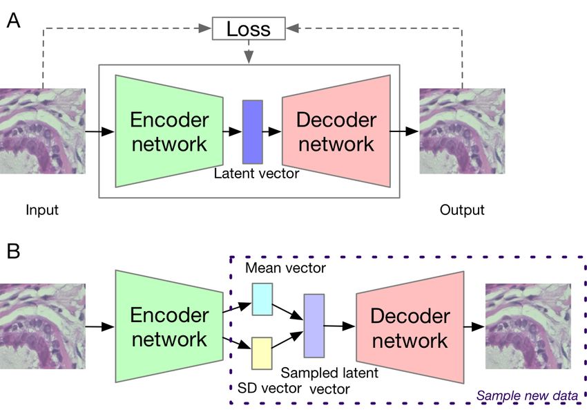
bioRxiv preprint first posted online Feb. 28, 2019; doi: http://dx.doi.org/10.1101/563601. The copyright holder for this preprint
 (which was not peer-reviewed) is the author/funder, who has granted bioRxiv a license to display the preprint in perpetuity.
                                    All rights reserved. No reuse allowed without permission.

             raw data since it can perform feature extraction and classification in an end-to-end manner, which
             determines the important high level features automatically. As for the structured data which have
             already gone through the feature extraction process, deep learning may not improve the performance
             significantly. However, it will not be worse than the conventional methods, such as support vector
             machine (SVM), as long as the hyper-parameters are carefully tunned. The applications of deep
             learning in those research directions and datasets are summarized in Table 2.
             Considering the great potential of deep learning in promoting the bioinformatic research, to facilitate
             the the development and application, in this review, we will first give a detailed and thorough
             introduction of deep learning (Section 2), from shallow neural networks to deep neural networks and
             their variants mentioned above, which are suitable for biological data analysis. After that, we provide
             a number of concrete examples (Section 3) with implementation available on Github, covering
             five bioinformatic research directions (sequence analysis, structure prediction and reconstruction,
             biomolecule property and function prediction, biomedical image processing and diagnosis, and
             biomolecular interaction prediction and systems biology) and all the four types of data (1D sequences,
             2D images and profiles, graphs, and preprocessed data). In terms of network types, those examples
             will cover fully connected neural networks, standard convolutional neural networks (CNN) [72],
             recurrent neural networks (RNN) [103], residual networks (ResNet) [53], generative adversarial
             networks (GAN) [43], variational autoencoder (VAE) [30], and graph convolutional neural networks
             (GCN) [69]. After those concrete examples, we will discuss the potential issues which researchers may
             encounter when using deep learning and the corresponding possible solutions (Section 4), including
             overfitting (Setion 4.2), data issues (Section 4.1 and 4.3), interpretability (Section 4.4), uncertainty
             scaling (Section 4.5), catastrophic forgetting (Section 4.6) and model compression (Section 4.7).
             Notice that there are a number of other review papers available, introducing the applications of
             deep learning in bioinformatics, biomedicine and healthcare [82, 5, 104, 98, 65, 18, 164, 36, 155],
             which are summarized in Table 3. Despite their comprehensive survey of recent applications of deep
             learning methods to the bioinformatics field and their insightful points about the future research
             direction combining deep learning and biology, seldom have those reviews introduced how those
             algorithms work step-by-step or provided tutorial type of reviews to bridge the gap between the
             method developers and the end users in biology. Biologists, who do not have strong machine learning
             background and want incorporate the deep learning method into their data analysis pipelines, may
             want to know exactly how those algorithms work, avoiding the pitfalls that people usually encounter
             when adopting deep learning in data analytics. Thus, complementary to the previous reviews, in
             this paper, we provide both the exoteric introduction of deep learning, and concrete examples and
             implementations of its representative applications in bioinformatics, to facilitate the adaptation of deep
             learning into biological data analysis pipeline. This review is in tutorial-style. For the completeness
             of this review, we also surveyed the related works in recent years, as shown in Table 2, as well as the
             obstacles and corresponding solutions when using deep learning (Section 4).

             2 From shallow neural networks to deep learning

             In this section, we will first introduce the form of a shallow neural network and its core components
             (Section 2.1). After that, we introduce the key components of the standard CNN and RNN (Section
             2.2). Since the standard CNN and RNN have been improved greatly over the past few years, we will
             also introduce several state-of-the-art architectures (Section 2.3), including ResNet, DenseNet and
             SENet [58]. After introducing the architecture for regular 1D and 2D data, we introduce graph neural
             networks for handling network data (Section 2.4). Then, we introduce two important generative
             models (Section 2.5), GAN and VAE, which can be useful for biomedical image processing and
             drug design. Finally, we give an overview of the currently available frameworks, which make the
             application of deep learning quite handy, for building deep learning models (Section 2.6). Notice that
             all the architectures and models are further illustrated and supported by the examples in Section 3.
             One can find the link between Section 2 and Section 3 with Table 4.

             2.1 Shallow neural networks and their components

             Fig. 1 shows the major components of a shallow neural network. In general, the whole network
             is a mapping function. Each subnetwork is also a mapping function. Taking the first hidden node
             as an example, which is shown in Fig. 1 (A), this building block function mapping contains two

                                                                       4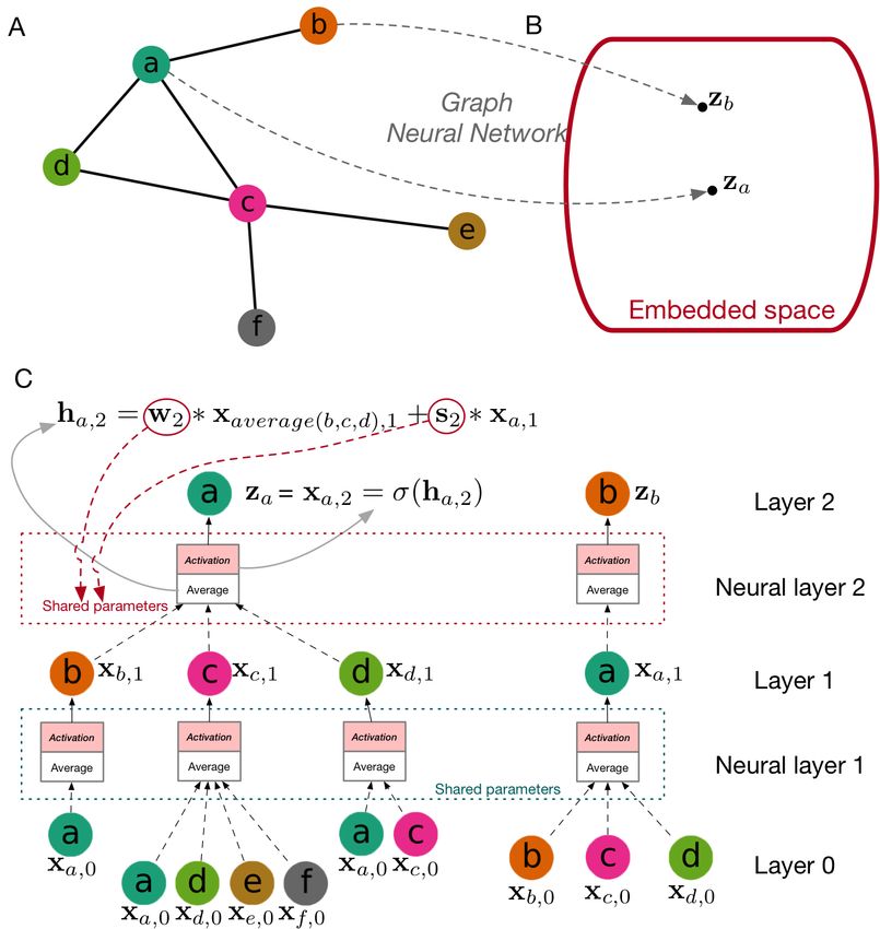
bioRxiv preprint first posted online Feb. 28, 2019; doi: http://dx.doi.org/10.1101/563601. The copyright holder for this preprint
 (which was not peer-reviewed) is the author/funder, who has granted bioRxiv a license to display the preprint in perpetuity.
                                    All rights reserved. No reuse allowed without permission.

             Figure 1: Illustration of a shallow neural network. (A) The operation within a single node. The input
             of the node will go through a linear transformation (dot product with the weight parameters and added
             with a bias) and a non-linear activation function to get the node output. (B) Illustration of the key
             components of a shallow neural network with one hidden layer. When training the model, we will
             run both the forward propagation and error back-propagation. Feeding the input value to the neural
             network and running forward propagation, we can obtain the output of the model, with which we can
             compare the target value and get the difference (loss or error). Then, we run error back-propagation
             and optimization to adjust the parameters of the model, making the output as close to the target value
             as possible. When the model is well-trained and we want to use the model, we will feed the input
             to the model and run forward propagation to obtain the output. Notice that in the hidden layer, the
             activation function is ReLU and the last output layer’s activation function is Softmax. The numbers
             in the parenthesis are the results of applying activation functions to the linear transformation outputs.

                                                                       5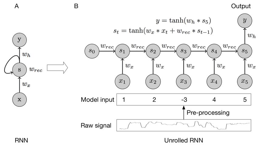
bioRxiv preprint first posted online Feb. 28, 2019; doi: http://dx.doi.org/10.1101/563601. The copyright holder for this preprint
 (which was not peer-reviewed) is the author/funder, who has granted bioRxiv a license to display the preprint in perpetuity.
                                    All rights reserved. No reuse allowed without permission.

                                            Table 3: Summaries of related review papers.
               Reference       Key words                Summary
               [82]            Machine learning, A review of machine learning tasks and related datasets in ge-
                               Genomic medicine         nomic medicine, not specific to deep learning
               [5]             Regulatory genomics, A review of deep learning’s applications in computational biology,
                               Cellular imaging        with an emphasis on regulatory genomics and cellular imaging
               [104]           Omics, Biomedical An general review of the CNN and RNN architectures, with the
                               imaging, Biomedical applications in omics, image processing and signal processing
                               signal processing
               [98]            Biomarker        devel- It discussed the key features of deep learning and a number of
                               opment, Transcrip- applications of it in biomedical studies
                               tomics
               [93]            Medical       imaging, It focuses on the applications of CNN in biomedical image pro-
                               CNN                      cessing, as well as the challenges in that field.
               [65]            Protein sequences       A tutorial-style review of using deep learning to handle sequence
                                                        data, with three application examples
               [18]            Biomedicine, Human It provides an review of the deep learning applications in
                               disease                  biomedicine, with comprehensive discussion of the obstacles
                                                       when using deep learning
               [164]           Biomedicine, Model It discusses the history and advantage of deep learning, arguing
                               flexibility              the potential of deep learning in biomedicine
               [36]            Healthcare, End-to- It discusses how techniques in computer vision, natural language
                               end system               processing, reinforcement learning can be used to build health
                                                        care system.
               [155]           High-performance         It discusses the applications of artificial intelligence into medicine,
                               system, Artificial in- as well as the potential challenges.
                               telligence, Medicine
               [17]            Model compression, A review of methods in compressing deep learning models and
                               Acceleration             reducing the computational requirements of deep learning meth-
                                                        ods.
               [111]           Catastrophic forget- A survey of incremental learning in neural network, discussing
                               ting,      Incremental how to incorporate new information into the model
                               learning
               [12]            Class imbalance          It investigates the impact of data imbalance to deep learning
                                                        model’s performance, with a comparison of frequently used tech-
                                                        niques to alleviate the problem
               [74]            Overfitting, Regular- A systematic review of regularization methods used to combat
                               ization                  overfitting issue in deep learning
               [195]           Interpretability,        It revisits the visualization of CNN representations and methods
                               Visual interpretation    to interpret the learned representations, with an perspective on
                                                        explainable artificial intelligence
               [153]           Transfer      learning, It reviews the transfer learning methods in deep learning field,
                               Data shortage            dealing with the data shortage problem
               [92]            Model interpretabil- A comprehensive discussion of the interpretability of machine
                               ity                      learning models, from the definition of interpretability to model
                                                        properties

             components, a linear transformation w*x and a non-linear one δ(z). By aggregating multiple building
             block functions into one layer and stacking two layers, we obtain the network shown in Fig. 1 (B),
             which is capable of expressing a nonlinear mapping function with a relatively high complexity.
             When we train a neural network to perform classification, we are training the neural network into a
             certain non-linear function to express (at least approximately) the hidden relationship between the
             features x and the label ŷ. In order to do so, we need to train the parameters w, making the model fit
             the data. The standard algorithm to do so is forward-backward propagation. After initializing the
             network parameters randomly, we run the network to obtain the network output (forward propagation).
             By comparing the output of the model and the ground truth label, we can compute the difference

                                                                       6
bioRxiv preprint first posted online Feb. 28, 2019; doi: http://dx.doi.org/10.1101/563601. The copyright holder for this preprint
(which was not peer-reviewed) is the author/funder, who has granted bioRxiv a license to display the preprint in perpetuity.
All rights reserved. No reuse allowed without permission.
(‘loss’ or ‘error’) between the two with a certain loss function. Using the gradient chain rule, we
can back-propagate the loss to each parameter and update the parameter with certain update rule
(optimizer). We will run the above steps iteratively (except for the random initialization) until the
model converges or reaches a pre-defined number of iterations. After obtaining a well-trained neural
network model, when we perform testing or use it, we will only run the forward propagation to obtain
the model output given the input.
From the above description, we can conclude that multiple factors in different scales can influence
the model’s performance. Starting from the building block shown in Fig. 1 (A), the choice of the
activation function can influence the model’s capacity and the optimization steps greatly. Currently,
the most commonly used activation functions are ReLU, Leaky ReLU, SELU, Softmax, TanH.
Among them, ReLU is the most popular one for the hidden layers and the Softmax is the most popular
one for the output layer. When combining those building blocks into a neural network, we need to
determine how many blocks we want to aggregate in one layer. The more nodes we put into the
neural network, the higher complexity the model will have. If we do not put enough nodes, the model
will be too simple to express the complex relationship between the input and the output, which results
in underfitting. If we put too many nodes, the model will be so complex that it will even express the
noise in the data, which causes overfitting. We need to find the balance when choosing the number
of nodes. After building the model, when we start training the model, we need to determine which
loss function we want to use and which optimizer we prefer. The commonly used loss functions
are cross-entropy for classification and mean squared error for regression. The optimizers include
stochastic gradient descent (SGD), Momentum, Adam [68] and RMSprop. Typically, if users are
not very familiar with the problem, Adam is recommended. If users have clear understanding of the
problem, Momentum with learning rate decay is a better option.
2.2 Legendary deep learning architectures: CNN and RNN
2.2.1 Legendary convolutional neural networks
Although the logic behind the shallow neural network is very clear, there are two drawbacks of
shallow neural networks. Firstly, the number of parameters is enormous: consider one hidden layer
having N1 nodes and the subsequent output layer containing N2 nodes, then, we will have N1 ∗ N2
parameters between those two layers. Such a large number of parameters can cause serious overfitting
issue and slow down the training and testing process. Secondly, the shallow neural network considers
each input feature independently, ignoring the correlation between input features, which is actually
common in biological data. For example, in a DNA sequence, a certain motif may be very important
for the function of that sequence [3]. Using the shallow network, however, we will consider each
base within the motif independently, instead of the motif as a whole. Although the large amount
of parameters may have the capability of capturing that information implicitly, a better option is
to incorporate that explicitly. To achieve that, the convolution neural network has been proposed,
which has two characteristics: local connectivity and weight sharing. We show the structure of
a legendary convolutional neural network in Fig. 2. Fig. 2 (B) shows the data flow logic of a
typical convolutional neural network, taking a chunk of Nanopore raw signals as input and predicting
whether the corresponding DNA sequence is methylated or not. The Nanopore raw signals are already
1D numerical vectors, which are suitable for being fed into a neural network (in terms of string
inputs, such as DNA sequences and protein sequences in the fasta format, which are common in
bioinformatics, the encoding will be discussed in Section 3). After necessary pre-processing, such
as denoising and normalization, the data vector will go through several (N ) convolutional layers
and pooling layers, after which the length of the vector becomes shorter but the number of channels
increases (different channels can be considered to represent the input sequence from different aspects,
like the RGB channels for an image). After the last pooling layer, the multi-channel vector will be
flatten into a single-channel long vector. The long vector fully connects with the output layer with a
similar architecture shown in Fig. 1.
Fig. 2 (A) shows the convolutional layer within CNN in more details. As shown in the figure, for
each channel of the convolutional layer output, we have one weight vector. The length of this vector
is shorter than the input vector. The weight vector slides across the input vector, performing inner
product at each position and obtaining the convolution result. Then, an activation function is applied
to the convolution result elementwisely, resulting in the convolutional layer output. Notice that each
element of the output is only related to a certain part of the input vector, which is referred as local
7bioRxiv preprint first posted online Feb. 28, 2019; doi: http://dx.doi.org/10.1101/563601. The copyright holder for this preprint
(which was not peer-reviewed) is the author/funder, who has granted bioRxiv a license to display the preprint in perpetuity.
All rights reserved. No reuse allowed without permission.
Figure 2: Illustration of a convolution neural network. (A) The convolutional layer operation. The
input goes through a convolution operation and a non-linear activation operation to obtain the output.
Those two operations can be repeated X times, so the output can have X channels. (B) The general
data flow of a convolutional neural network. After pre-processing, the data usually go through
convolutional layers, pooling layers, flatten layers, and fully connected layers to produce the final
output. As for the other components, such as back-propagation and optimization, it is the same as the
shallow neural network. (C) The max pooling operation. (D) The flatten operation, which converts a
vector with multiple channels into a long vector with only one channel.
8bioRxiv preprint first posted online Feb. 28, 2019; doi: http://dx.doi.org/10.1101/563601. The copyright holder for this preprint
(which was not peer-reviewed) is the author/funder, who has granted bioRxiv a license to display the preprint in perpetuity.
All rights reserved. No reuse allowed without permission.
Figure 3: Illustration of a recurrent neural network. (A) A typical rolled RNN representation. (B) An
easy-to-understand unrolled RNN representation. The model processes the input element by element
which enables the model to capture the temporal information within the input.
connectivity. Besides, unlike the structure in Fig. 1, in convolutional layers, different parts of the
input vector share the same weight vector when performing the sliding inner product (convolution),
which is the weight-sharing property. Under this weight-sharing and local connectivity setting, we can
find that the weight vector serves as a pattern or motif finder, which satisfies our original motivation
of introducing this architecture. Notice that the original input is a vector with one channel. After
the first convolutional layer, the input of the next convolutional layer usually has more than one
channel. Correspondingly, the weight vector should have the same number of channels to make the
convolutional operation feasible. For example, in Fig. 2 (B), the output of the first convolutional
layer has 4 channels. Accordingly, the filters of the next convolutional layer should have 4 channels.
If the filter length is the same as what is shown in Fig. 2 (A), which is 2, the filters should have the
dimensionality as 2 by 4. If the output of the second convolutional layer has 16 channels, we should
have 16 filters, one for each output channel. Considering all the above factors, the filter tensor of the
second convolutional layer should have a dimensionality of 2*4*16, which is a 3D tensor. For image
inputs, we usually have a 4D tensor as the filter of each convolutional layer, whose four dimensions
correspond to filter length, filter width, input channels and output channels, respectively.
Fig. 2 (C) shows the max pooling operation. In the max pooling layer, each element of the output is
the maximum of the corresponding region in the layer input. Depending on the applications, people
can choose the pooling region size and steps (filter size and stride), or a different pooling method,
such as average pooling. This pooling layer enables the network to capture higher level and long
range property of the input vector, such as the long range interaction between the bases within the
corresponding DNA sequences of the input signals. Fig. 2 (D) shows the flatten layer. This operation
is straightforward, just concatenating the input vectors with multiple channels into a long vector with
only one channel to enable the downstream fully connected layer operation.
With the convolutional layers and the pooling layers, this neural network architecture is able to
capture the inputs’ property in different levels and at different scales, including both the local motif
and long range interaction.
9bioRxiv preprint first posted online Feb. 28, 2019; doi: http://dx.doi.org/10.1101/563601. The copyright holder for this preprint
(which was not peer-reviewed) is the author/funder, who has granted bioRxiv a license to display the preprint in perpetuity.
All rights reserved. No reuse allowed without permission.
2.2.2 Legendary recurrent neural networks
In addition to the spatial dependency within the input, we also need to consider the temporal or
order dependency in the input. For example, in DNA sequences, the order of motifs can influence
the function of the sequence chunk [120]. In a document, we need to consider the order of words
and sentences to categorize the document [94]. Similar to the case of spatial information, since
the shallow neural networks shown in Fig. 1 consider each element of the input independently, the
temporal information may also be lost. Recurrent neural networks are specifically designed to exploit
the temporal relationship within a sequential input. The basic structure of a recurrent neural network
is shown in Fig. 3. Let us consider an RNN with only one hidden recurrent cell, as shown in Fig.
3 (A). To explain how RNN works, we unroll the network into Fig. 3 (B), using the simplified
Nanopore raw signals as an example. As in CNN, we first perform necessary pre-processing, such
as normalization and denoising. Then the vector will be fed to the model element by element. The
hidden recurrent cell has an initial state, which is denoted as s0 and can be initialized randomly. After
taking the first value, the recurrent node is updated, considering the previous state s0 and x1 . Under
our setting, the update rule is s1 = tanh(wx ∗ x1 + wrec ∗ s0 ). When the second value comes in,
the node state is updated to s2 with the same rule. We repeat the above process until we consider
all the elements. Then the node information will be fed forward to make predictions, e.g., whether
the corresponding DNA sequence of the input Nanopore raw signals is methylated or not, with the
similar downstream structure in Fig. 1. Notice that wx and wrec are shared among all the time steps
or positions for that specific hidden recurrent node. Usually, one single recurrent node is not enough
to capture all the temporal information. Under that circumstance, we can increase the number of
recurrent nodes, each with its own pair of wx and wrec . For the last hidden layer, we can use a fully
connected layer to connect all the hidden recurrent nodes to the output node, like we is done in the
CNN scenario. In terms of training and optimization, it is the same as the case in shallow neural
networks. We will run error back-propagation to make the weight parameters fit the training data and
perform prediction afterwards.
2.3 State-of-the-art deep architectures
In the past several years, the above two legendary deep learning architectures have been improved
greatly. For convolutional neural networks, AlexNet [72], VGG [142], GoogleNet [21, 152], ResNet
[52, 53], ResNext [179], SENet [58], DenseNet [60] and DPN [16] have been proposed. For
recurrent neural networks, there are LSTM [39], Bi-RNN [44], GRU [23], Memory network [173]
and Attention network [162]. In Fig. 4, we exhibit some typical CNN architectures to deal with 2D
image data, showing the evolving of convolutional neural networks. In general, the more advanced
CNN architectures allow people to stack more layers, with the hope to extract more useful hidden
informations from the input data at the expense of more computational resources. For recurrent neural
networks, the more advanced architectures help people deal with the gradient vanishing or explosion
issue and accelerate the execution of RNN. However, how to parallelize RNN is still a big problem
under active investigation [187].
2.4 Graph neural networks
In this section, we briefly introduce graph neural networks [69, 48] to deal with network data, which is
a common data type in bioinformatics. Unlike the sequence and image data, network data are irregular:
a node can have arbitrary connection with other nodes. Although the data are complex, the network
information is very important for bioinformatics analysis, because the topological information and
the interaction information often have a clear biological meaning, which is a helpful feature for
perform classification or prediction. When we deal with the network data, the primary task is to
extract and encode the topological and connectivity information from the network, combining that
information with the internal property of the node [48]. For example, Fig. 5 (A) shows a protein-
protein interaction network and each node in the network represents a protein. In addition to the
interaction information, each protein has some internal properties, such as the sequence information
and the structure information. If we want to predict whether a protein in the network is an enzyme,
both the interaction information and the internal properties can be helpful. So, what we need to do
is to encode the protein in the network in a way that we consider both the network information and
the properties, which is known as an embedding problem. In other words, we embed the network
data into a regular space, as shown in Fig. 5 (B), where the original topological information is
10bioRxiv preprint first posted online Feb. 28, 2019; doi: http://dx.doi.org/10.1101/563601. The copyright holder for this preprint
(which was not peer-reviewed) is the author/funder, who has granted bioRxiv a license to display the preprint in perpetuity.
All rights reserved. No reuse allowed without permission.
Figure 4: Illustration of different convolutional neural network architectures. (A) The convolutional
neural network building block. ‘Conv’ represents the convolutional operation. ‘ReLU’ represents
the activation function. (B) The legendary convolutional neural network with two convolutional
layers. Each convolutional layer contains ‘Conv’, ‘BN’, and ‘ReLU’, where ‘BN’ represents batch
normalization, which accelerates the training process [61]. (C) The residual block of a residual
network [53]. In addition to the legendary convolutional layers along the data flow process, there is a
shortcut between the input and the output, which adds the input elementwisely to the convolutional
layer output to obtain the residual block output. In fact, unlike the architecture in (B), where the
convolutional layers are used to model the mapping between the input and the output, here in (C),
those convolutional layers are used to model the residual between the input and the residual block
output. (D) The building block of SENet [58]. This architecture further improves the residual block,
which introduces the idea of Attention [162] into the residual network. In (C), different channels of
the output are considered of equal importance. However, in reality, some channels can contain more
information and thus more important. The SENet block considers that, learning a scaling function and
applying the scaling function to the output of the residual block to obtain the SENet block output. In
the figure, ‘GP’ represents global pooling; ‘FC’ represents a fully connected layer. (E) The DenseNet
block [60]. Unlike (C,D), which have the elementwise addition shortcut, DenseNet block’s shortcut
is stacking operation (‘stack’ in the figure), which concatenates the original input to the output of a
certain convolutional layer along the channel dimension. This block can result in outputs with a large
number of channels, which is proved to be a better architecture.
preserved. For an embedding problem, the most important thing is to aggregate information from a
node’s neighbor nodes [48]. Graph convolutional neural networks (GCN), shown in Fig. 5 (C) are
designed for such a purpose. Suppose we consider a graph neural network with two layers. For each
node, we construct a neighbor tree based on the network (Fig. 5 (C) shows the tree constructed for
node a and node b). Then we can consider layer 0 as the neural network inputs, which can be the
proteins’ internal property encoding in our setting. Then, node a’s neighbors aggregate information
from their neighbors, followed by averaging and activating, to obtain their level 1 representation.
After that, node a collects information from its neighbors’ level 1 representation to obtain its level 2
representation, which is the neural networks’ output embedding result in this example.
Take the last step as an example, the information collection (average) rule is: ha,2 = w2 ∗
xaverage(b,c,d),1 + s2 ∗ xa,1 , where xaverage(b,c,d),1 is the average of node b,c,d’s level 1 embed-
ding, xa,1 is node a’s level 1 embedding, and w2 and s2 are the trainable parameters. To obtain the
level 2 embedding, we apply an activation function to the average result: xa,2 = σ(ha,2 ). Notice that
between different nodes, the weights within the same neural layer are shared, which means the graph
neural network can be generalized to previously unseen network of the same type. To train the graph
neural network, we need to define a loss function, with which we can use the back-propagation to
perform optimization. The loss function can be based on the similarity, that is, similar nodes should
11bioRxiv preprint first posted online Feb. 28, 2019; doi: http://dx.doi.org/10.1101/563601. The copyright holder for this preprint
(which was not peer-reviewed) is the author/funder, who has granted bioRxiv a license to display the preprint in perpetuity.
All rights reserved. No reuse allowed without permission.
Figure 5: Illustration of a graph neural network. (A) A typical example of graph data. (B) The
embedding space. In this embedding space, each data point is represented by a vector while the
original topological information in (A) is preserved in that vector. (C) The graph neural network for
embedding the network in (A). We use node a and b as examples. The internal properties of each node
are considered as the original representations. In each layer, the nodes aggregate information from
their neighbors and update the representations with averaging and activation function. The output of
layer 2 are considered as the embedding result in this example. Notice that the parameters within the
same layer between different trees are shared so this method can be generalized to previously unseen
graph of the same type.
12bioRxiv preprint first posted online Feb. 28, 2019; doi: http://dx.doi.org/10.1101/563601. The copyright holder for this preprint
(which was not peer-reviewed) is the author/funder, who has granted bioRxiv a license to display the preprint in perpetuity.
All rights reserved. No reuse allowed without permission.
Figure 6: Illustration of GAN. In GAN, we have a pair of networks competing with each other at the
same time. The generator network is responsible for generating new data points (enzyme sequences
in this example). The discriminator network tries to distinguish the generated data points from the
real data points. As we train the networks, both models’ abilities are improved. The ultimate goal
is to make the generator network able to generate enzyme sequences that are very likely to be real
ones that have not been discovered yet. The discriminator network can use the architectures in Fig.
4. As for the generator network, the last layer should have the same dimensionality as the enzyme
encoding.
have similar embeddings [45, 116, 127]. Or we can use a classification task directly to train the GCN
in a discriminative way [33, 69, 202]: we can stack a shallow neural network, CNN or RNN, on the
top of GNN, taking the embedding output of the GCN as input and training the two networks at the
same time.
2.5 Generative models: GAN and VAE
In this section, we introduce two generative networks, GAN [43] and VAE [30], which can be
useful for biological and biomedical image processing [183, 90, 137] and protein or drug design
[132, 119, 122]. Unlike supervised learning, using which we perform classification or regression,
such as the task of predicting whether a protein is an enzyme, the generative models belong to
unsupervised learning, which cares more about the intrinsic properties of the data. With generative
models, we want to learn the data distribution and generate new data points with some variations. For
example, given a set of protein sequences which are enzymes as the training dataset, we want to train
a generative model which can generate new protein sequences that are also enzymes.
Generative adversarial networks (GAN) have achieved great success in the computer vision field [43],
such as generating new semantic images [43], image style transfer [62, 200], image inpainting [186]
and image super-resolution [78, 90]. As shown in Fig. 6, instead of training only one neural network,
GAN trains a pair of networks which compete with each other. The generator network is the final
productive neural network which can produce new data samples (novel enzyme sequences in this
example) while the discriminator network distinguishes the designed enzyme sequences from the real
ones to push the generator network to produce protein sequences that are more likely to be enzyme
sequences instead of some random sequences. Both of the generator network and the discriminator
network can be the networks mentioned in Section 2.2.1. For the generator network, the last layer
needs to be redesigned to match the dimensionality of an enzyme sequence encoding.
13bioRxiv preprint first posted online Feb. 28, 2019; doi: http://dx.doi.org/10.1101/563601. The copyright holder for this preprint
(which was not peer-reviewed) is the author/funder, who has granted bioRxiv a license to display the preprint in perpetuity.
All rights reserved. No reuse allowed without permission.
Figure 7: (A) Illustration of autoencoder, which is composed of encoder and decoder. The encoder
network compresses the input into the latent vector and the decoder network reconstructs data from
the latent vector. The loss is usually defined as the difference between the input and the decoder
output. Notice that the latent vector’s dimensionality is much smaller than the original input. (B)
Illustration of VAE. To enable the network to sample new data points, instead of mapping the inputs
into fixed latent vectors, VAE maps the inputs into a distribution in the latent space with the encoder
network. When we need to sample new data, we can first sample the latent vector from the distribution
and then generate the data using the decoder network with the sampled latent vector as input.
To introduce variational autoencoder, let us first go through autoencoder, which is shown in Fig.
7 (A). The autoencoder is usually used to encode high dimensional input data, such as an image,
into a much lower dimensional representation, which can store the latent information of the data
distribution. It contains two parts, the encoder network and the decoder network. The encoder
network can transform the input data into a latent vector and the decoder network can reconstruct the
data from the latent vector with the hope that the reconstructed image is as close to the original input
as possible. Autoencoder is very convenient for dimensionality reduction. However, we cannot use
it to generate new data which are not in the original input. Variational antoencoder overcomes the
bottleneck by making a slight change to the latent space. Instead of mapping the input data to one
exact latent vector, we map the data into a low dimensional data distribution, as shown in Fig. 7 (B).
With the latent distribution, when we need to sample new data points, we can first sample the latent
vector from the latent vector distribution and then construct the new data using the decoder network.
2.6 Frameworks
Building the whole network and implementing the optimizers completely from scratch will be
very tedious and time-consuming. Fortunately, there are a number of handy frameworks available,
which can accelerate the process of building networks and training the model. After evolving for
several years, the following frameworks are commonly used, and actively developed and maintained:
Tensorflow [1], Pytorch [112], Caffe2, MXNet [13], CNTK [138] and PaddlePaddle. Another famous
warpper of Tensorflow is Keras, with which one can build a model in several lines of code. It is very
convenient and easy-to-use, although it lacks the flexibility provided by Tensorflow, using which one
can control almost every single detail.
14bioRxiv preprint first posted online Feb. 28, 2019; doi: http://dx.doi.org/10.1101/563601. The copyright holder for this preprint
(which was not peer-reviewed) is the author/funder, who has granted bioRxiv a license to display the preprint in perpetuity.
All rights reserved. No reuse allowed without permission.
Table 4: Summary of the examples.
Example Model Data type Research direction Task
Enzyme function pre- DNN Structured Biomolecular function pre- Classification
diction diction
Gene expression re- DNN Structured Biomolecular property pre- Regression
gression diction
RNA-protein binding CNN 1D data Sequence analysis Classification
sites prediction
DNA sequence func- CNN, 1D data Sequence analysis Classification
tion prediction RNN
Biomedical image ResNet 2D data Biomedical image process- Classification
classification ing
Protein interaction GCN Graph Biomolecule interaction pre- Embedding, Classifi-
prediction diction cation
Biology image super- GAN 2D image Structure reconstruction Data generation
resolution
Gene expression data VAE 2D data Systems biology DR, Data generation
embedding
3 Applications of deep learning in bioinformatics
This section provides eight examples. Those examples are carefully selected, typical examples of
applying deep learning methods into important bioinformatic problems, which can reflect all of the
above discussed research directions, models, data types, and tasks, as summarized in Table 4. In terms
of research directions, Sections 3.3 and 3.4 are related to sequence analysis; Section 3.7 is relevant
to structure prediction and reconstruction; Section 3.1 is about biomolecular property and function
prediction; Sections 3.7 and 3.5 are related to biomedical image processing and diagnosis; Sections
3.2, 3.6, and 3.8 are relevant to biomolecule interaction prediction and systems biology. Regarding
the data type, Sections 3.1 and 3.2 use structured data; Sections 3.3 and 3.4 use 1D sequence data;
Sections 3.5, 3.7, and 3.8 use 2D image or profiling data; Section 3.6 uses graph data.
From the deep learning point of view, those examples also cover a wide range of deep learning
models: Sections 3.1 and 3.2 use deep fully connected neural networks; Section 3.3 uses CNN;
Section 3.4 combines CNN with RNN; Section 3.6 uses GCN; Section 3.5 uses ResNet; Section
3.7 uses GAN; Section 3.8 uses VAE. We cover both supervised learning, including classification
(Sections 3.1, 3.3, 3.4, and 3.5) and regression (Section 3.2), and unsupervised learning (Sections 3.6,
3.7, and 3.8). We also introduce transfer learning using deep learning briefly (Section 3.5).
3.1 Identifying enzymes using multi-layer neural networks
Enzymes are one of the most important types of molecules in human body, catalyzing biochemical
reactions in vivo. Accurately identifying enzymes and predicting their function can benefit various
fields, such as biomedical diagnosis and industrial bio-production [85]. In this example, we show how
to identify enzyme sequences based on sequence information using deep learning based methods.
Usually, a protein sequence is represented by a string (such as, ‘MLAC...’), but deep learning models,
as mathematical models, take numerical values as inputs. So before building the deep learning model,
we need to first encode the protein sequences into numbers. The common ways of encoding a protein
sequences are discussed in [85]. In this example, we use a sparse way to encode the protein sequences,
the functional domain encoding. For each protein sequence, we use HMMER [34] to search it against
the protein functional domain database, Pfam [37]. If a certain functional domain is hit, we encode
that domain as 1, otherwise 0. Since Pfam has 16306 functional domains, we have a 16306D vector,
composed of 0s and 1s, to encode each protein sequence. Because the dimensionality of the feature
is very high, the traditional machine learning method may encounter the curse of dimensionality.
However, the deep learning method can handle the problem quite well. As for the dataset, we use
the dataset from [85], which contains 22168 enzyme sequences and 22168 non-enzyme protein
sequences, whose sequence similarity is under 40% within each class.
15bioRxiv preprint first posted online Feb. 28, 2019; doi: http://dx.doi.org/10.1101/563601. The copyright holder for this preprint
(which was not peer-reviewed) is the author/funder, who has granted bioRxiv a license to display the preprint in perpetuity.
All rights reserved. No reuse allowed without permission.
In our implementation, we adopt a similar architecture as Fig. 1, but with much more nodes and
layers. We use ReLU as the activation function, cross-entropy loss as the loss function, and Adam as
the optimizer. We utilize dropout, batch normalization and weight decay to prevent overfitting. With
the help of Keras, we build and train the model in 10 lines. Training the model on a Titan X for 2
minutes, we can reach around 94.5% accuracy, which is very close to the state-of-the-art performance
[85]. Since bimolecular function prediction and annotation is one of the main research directions of
bioinformatics, researchers can easily adopt this example and develop the applications for their own
problems.
3.2 Gene expression regression
Gene expression data are one of the most common and useful data types in bioinformatics, which can
be used to reflect the cellular changes corresponding to different physical and chemical conditions and
genetic perturbations [161, 14]. However, the whole genome expression profiling can be expensive.
To reduce the cost of gene profiling, realizing that different genes’ expression can be highly correlated,
researchers have developed an affordable method of only profiling around 1000 carefully selected
landmark genes and predicting the expression of the other target genes based on computational
methods and landmark gene expression [32, 14]. Previously, the most commonly used method is
linear regression. Recently, [14] showed that deep learning based regression can outperform the
linear regression method significantly since it considered the non-linear relationship between genes’
expression.
In this example, we use deep learning method to perform gene expression prediction as in [14],
showing how to perform regression using deep learning. We use the Gene Expression Omnibus
(GEO) dataset from [14], which has already gone through the standard normalization procedure. For
the deep learning architecture, we use a similar structure as in Section 3.1. However, the loss function
for this regression problem is very different from the classification problem in Section 3.1. As we
discussed in Section 2.1, for classification problems, we usually use cross-entropy loss, while for
the regression problem, we use the mean squared error as the loss function. Besides, we also change
the activation function of the last layer from Softmax to TanH for this application. Using Keras, the
network can be built and trained in 10 lines. Trained on a Titan X card for 2 mins, it can outperform
the linear regression method by 4.5% on a randomly selected target gene.
Our example code can be easily used and adopted for other bioinformatics regression problems. On
the other hand, if one is sure about the regression target value range, then the target range can be
divided into several bins and the regression problem is converted into a classification problem. With
the classification problem in hand, people can use the classification examples introduced in the other
sections.
3.3 RNA-protein binding sites prediction with CNN
RNA-binding proteins (RBP) play an important role in regulating biological processes, such as gene
regulation [40, 110]. Understanding their behaviors, for example, their binding site, can be helpful
for cuing RBP related diseases. With the advancement of high-throughput technologies, such as
CLIP-seq, we can verify the RBP binding sites in batches [83]. However, despite its efficiency,
those high-throughput technologies can be expensive and time-consuming. Under that circumstance,
machine learning based computational methods, which are fast and affordable, can be helpful to
predict the RBP binding site [110].
In fact, the deep learning methods are especially suitable for this kind of problems. As we know, RBP
can have sequence preference, recognizing specific motifs and local structures and binding to those
points specifically [123]. On the other hand, as we discussed in Section 2.2.1, CNN are especially
good at detecting special patterns in different scales. Previous studies have shown the power of CNN
in finding motifs [110, 25].
In this example, we show how to predict the RBP binding site using CNN, with the data from [110].
Specifically, the task is to predict whether a certain RBP, which is fixed for one model, can bind to a
certain given RNA sequence, that is, a binary classification problem. We use one-hot encoding to
convert the RNA sequence strings of ‘AUCG’ into 2D tensors. For example, for ‘A’, we use a vector
(1, 0, 0, 0) to represent it; for ‘U’, we use a vector (0, 1, 0, 0) to represent it. Concatenating those 1D
vectors into a 2D tensor in the same order as the original sequence, we obtain the one-hot encoding
16You can also read