Machine Learning on Graphs: A Model and Comprehensive Taxonomy - arXiv.org
←
→
Page content transcription
If your browser does not render page correctly, please read the page content below
Machine Learning on Graphs:
                                                                       A Model and Comprehensive Taxonomy
                                         Ines Chami* † , Sami Abu-El-Haija‡ , Bryan Perozzi†† , Christopher R采 , and Kevin Murphy††

                                                                   †
                                                                       Stanford University, Institute for Computational and Mathematical Engineering
                                                                             ‡
                                                                               University of Southern California, Information Sciences Institute
arXiv:2005.03675v2 [cs.LG] 18 Jan 2021

                                                                                  ‡‡
                                                                                     Stanford University, Department of Computer Science
                                                                                                      ††
                                                                                                         Google Research
                                                  {chami,chrismre}@cs.stanford.edu, sami@haija.org, bperozzi@acm.org, kpmurphy@google.com

                                                                                                   January 19, 2021

                                                                                                            Abstract
                                                 There has been a surge of recent interest in graph representation learning (GRL). GRL methods have generally
                                             fallen into three main categories, based on the availability of labeled data. The first, network embedding, focuses on
                                             learning unsupervised representations of relational structure. The second, graph regularized neural networks, lever-
                                             ages graphs to augment neural network losses with a regularization objective for semi-supervised learning. The third,
                                             graph neural networks, aims to learn differentiable functions over discrete topologies with arbitrary structure. How-
                                             ever, despite the popularity of these areas there has been surprisingly little work on unifying the three paradigms.
                                             Here, we aim to bridge the gap between network embedding, graph regularization and graph neural networks. We
                                             propose a comprehensive taxonomy of GRL methods, aiming to unify several disparate bodies of work. Specifically,
                                             we propose the G RAPH EDM framework, which generalizes popular algorithms for semi-supervised learning (e.g.
                                             GraphSage, GCN, GAT), and unsupervised learning (e.g. DeepWalk, node2vec) of graph representations into a single
                                             consistent approach. To illustrate the generality of G RAPH EDM, we fit over thirty existing methods into this frame-
                                             work. We believe that this unifying view both provides a solid foundation for understanding the intuition behind these
                                             methods, and enables future research in the area.

                                         * Work   partially done during an internship at Google Research.

                                                                                                               1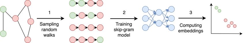
Contents
1   Introduction                                                                                                                                                                                     3

2   Preliminaries                                                                                                                                                                                    5
    2.1 Definitions . . . . . . . . . . . . . . . . . . . . . . . . .                                .   .   .   .   .   .   .   .   .   .   .   .   .   .   .   .   .   .   .   .   .   .   .   .   5
    2.2 The generalized network embedding problem . . . . . .                                        .   .   .   .   .   .   .   .   .   .   .   .   .   .   .   .   .   .   .   .   .   .   .   .   7
         2.2.1 Node features in network embedding . . . . . .                                        .   .   .   .   .   .   .   .   .   .   .   .   .   .   .   .   .   .   .   .   .   .   .   .   7
         2.2.2 Transductive and inductive network embedding .                                        .   .   .   .   .   .   .   .   .   .   .   .   .   .   .   .   .   .   .   .   .   .   .   .   7
         2.2.3 Positional vs structural network embedding . . .                                      .   .   .   .   .   .   .   .   .   .   .   .   .   .   .   .   .   .   .   .   .   .   .   .   8
         2.2.4 Unsupervised and supervised network embedding                                         .   .   .   .   .   .   .   .   .   .   .   .   .   .   .   .   .   .   .   .   .   .   .   .   8

3   A Taxonomy of Graph Embedding Models                                                                                                                                                              8
    3.1 The G RAPH EDM framework . . . . . . . . . . . . . . . . . . . . . . . . . . . . . . . . . . . . . . .                                                                                        8
    3.2 Taxonomy of objective functions . . . . . . . . . . . . . . . . . . . . . . . . . . . . . . . . . . . . .                                                                                    10
    3.3 Taxonomy of encoders . . . . . . . . . . . . . . . . . . . . . . . . . . . . . . . . . . . . . . . . . .                                                                                     11

4   Unsupervised Graph Embedding                                                                                                                                                                     11
    4.1 Shallow embedding methods . . . . . . . . . . . . . . . .                                        .   .   .   .   .   .   .   .   .   .   .   .   .   .   .   .   .   .   .   .   .   .   .   13
        4.1.1 Distance-based: Euclidean methods . . . . . . . .                                          .   .   .   .   .   .   .   .   .   .   .   .   .   .   .   .   .   .   .   .   .   .   .   13
        4.1.2 Distance-based: Non-Euclidean methods . . . . .                                            .   .   .   .   .   .   .   .   .   .   .   .   .   .   .   .   .   .   .   .   .   .   .   15
        4.1.3 Outer product-based: Matrix factorization methods                                          .   .   .   .   .   .   .   .   .   .   .   .   .   .   .   .   .   .   .   .   .   .   .   16
        4.1.4 Outer product-based: Skip-gram methods . . . . .                                           .   .   .   .   .   .   .   .   .   .   .   .   .   .   .   .   .   .   .   .   .   .   .   17
    4.2 Auto-encoders . . . . . . . . . . . . . . . . . . . . . . . .                                    .   .   .   .   .   .   .   .   .   .   .   .   .   .   .   .   .   .   .   .   .   .   .   19
    4.3 Graph neural networks . . . . . . . . . . . . . . . . . . .                                      .   .   .   .   .   .   .   .   .   .   .   .   .   .   .   .   .   .   .   .   .   .   .   20

5   Supervised Graph Embedding                                                                                                                                                                       22
    5.1 Shallow embedding methods . . . . . . . . . . . . . . . . . . . .                                                .   .   .   .   .   .   .   .   .   .   .   .   .   .   .   .   .   .   .   22
    5.2 Graph regularization methods . . . . . . . . . . . . . . . . . . . .                                             .   .   .   .   .   .   .   .   .   .   .   .   .   .   .   .   .   .   .   23
        5.2.1 Laplacian . . . . . . . . . . . . . . . . . . . . . . . . . .                                              .   .   .   .   .   .   .   .   .   .   .   .   .   .   .   .   .   .   .   23
        5.2.2 Skip-gram . . . . . . . . . . . . . . . . . . . . . . . . . .                                              .   .   .   .   .   .   .   .   .   .   .   .   .   .   .   .   .   .   .   24
    5.3 Graph convolution framework . . . . . . . . . . . . . . . . . . .                                                .   .   .   .   .   .   .   .   .   .   .   .   .   .   .   .   .   .   .   24
        5.3.1 The Graph Neural Network model and related frameworks                                                      .   .   .   .   .   .   .   .   .   .   .   .   .   .   .   .   .   .   .   25
        5.3.2 Graph Convolution Framework . . . . . . . . . . . . . .                                                    .   .   .   .   .   .   .   .   .   .   .   .   .   .   .   .   .   .   .   26
    5.4 Spectral Graph Convolutions . . . . . . . . . . . . . . . . . . . .                                              .   .   .   .   .   .   .   .   .   .   .   .   .   .   .   .   .   .   .   27
        5.4.1 Spectrum-based methods . . . . . . . . . . . . . . . . . .                                                 .   .   .   .   .   .   .   .   .   .   .   .   .   .   .   .   .   .   .   27
        5.4.2 Spectrum-free methods . . . . . . . . . . . . . . . . . . .                                                .   .   .   .   .   .   .   .   .   .   .   .   .   .   .   .   .   .   .   28
    5.5 Spatial Graph Convolutions . . . . . . . . . . . . . . . . . . . . .                                             .   .   .   .   .   .   .   .   .   .   .   .   .   .   .   .   .   .   .   30
        5.5.1 Sampling-based spatial methods . . . . . . . . . . . . . .                                                 .   .   .   .   .   .   .   .   .   .   .   .   .   .   .   .   .   .   .   30
        5.5.2 Attention-based spatial methods . . . . . . . . . . . . . .                                                .   .   .   .   .   .   .   .   .   .   .   .   .   .   .   .   .   .   .   31
    5.6 Non-Euclidean Graph Convolutions . . . . . . . . . . . . . . . .                                                 .   .   .   .   .   .   .   .   .   .   .   .   .   .   .   .   .   .   .   32

6   Applications                                                                                                                                                                                     32
    6.1 Unsupervised applications .      .   .   .   .   .   .   .   .   .   .   .   .   .   .   .   .   .   .   .   .   .   .   .   .   .   .   .   .   .   .   .   .   .   .   .   .   .   .   .   33
         6.1.1 Graph reconstruction      .   .   .   .   .   .   .   .   .   .   .   .   .   .   .   .   .   .   .   .   .   .   .   .   .   .   .   .   .   .   .   .   .   .   .   .   .   .   .   33
         6.1.2 Link prediction . . .     .   .   .   .   .   .   .   .   .   .   .   .   .   .   .   .   .   .   .   .   .   .   .   .   .   .   .   .   .   .   .   .   .   .   .   .   .   .   .   33
         6.1.3 Clustering . . . . . .    .   .   .   .   .   .   .   .   .   .   .   .   .   .   .   .   .   .   .   .   .   .   .   .   .   .   .   .   .   .   .   .   .   .   .   .   .   .   .   33
         6.1.4 Visualization . . . .     .   .   .   .   .   .   .   .   .   .   .   .   .   .   .   .   .   .   .   .   .   .   .   .   .   .   .   .   .   .   .   .   .   .   .   .   .   .   .   33
    6.2 Supervised applications . . .    .   .   .   .   .   .   .   .   .   .   .   .   .   .   .   .   .   .   .   .   .   .   .   .   .   .   .   .   .   .   .   .   .   .   .   .   .   .   .   34
         6.2.1 Node classification .     .   .   .   .   .   .   .   .   .   .   .   .   .   .   .   .   .   .   .   .   .   .   .   .   .   .   .   .   .   .   .   .   .   .   .   .   .   .   .   34
         6.2.2 Graph classification .    .   .   .   .   .   .   .   .   .   .   .   .   .   .   .   .   .   .   .   .   .   .   .   .   .   .   .   .   .   .   .   .   .   .   .   .   .   .   .   34

7   Conclusion and Open Research Directions                                                                                                                                                          34

                                                                                 2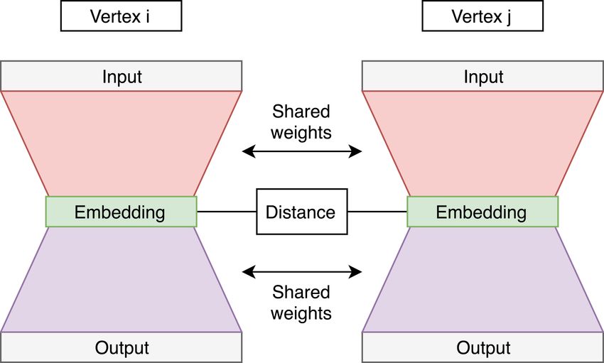
1    Introduction
Learning representations for complex structured data is a challenging task. In the last decade, many successful models
have been developed for certain kinds of structured data, including data defined on a discretized Euclidean domain.
For instance, sequential data, such as text or videos, can be modelled via recurrent neural networks, which can capture
sequential information, yielding efficient representations as measured on machine translation and speech recognition
tasks. Another example is convolutional neural networks (CNNs), which parameterize neural networks according to
structural priors such as shift-invariance, and have achieved unprecedented performance in pattern recognition tasks
such as image classification or speech recognition. These major successes have been restricted to particular types of
data that have a simple relational structure (e.g. sequential data, or data following regular patterns).
    In many settings, data is not nearly as regular: complex relational structures commonly arise, and extracting
information from that structure is key to understanding how objects interact with each other. Graphs are a universal
data structures that can represent complex relational data (composed of nodes and edges), and appear in multiple
domains such as social networks, computational chemistry [55], biology [127], recommendation systems [78], semi-
supervised learning [53], and others. For graph-structured data, it is challenging to define networks with strong
structural priors, as structures can be arbitrary, and can vary significantly across different graphs and even different
nodes within the same graph. In particular, operations like convolutions cannot be directly applied on irregular graph
domains. For instance in images, each pixel has the same neighborhood structure, allowing to apply the same filter
weights at multiple locations in the image. However in graphs, one can’t define an ordering of node since each
node might have a different neighborhood structure (Fig. 1). Furthermore, Euclidean convolutions strongly rely on
geometric priors (e.g. shift invariance) which don’t generalize to non-Euclidean domains (e.g. translations might not
even be defined on non-Euclidean domains).
    These challenges led to the development of Geometric Deep Learning (GDL) research which aims at applying
deep learning techniques to non-Euclidean data. In particular, given the widespread prevalence of graphs in real-
world applications, there has been a surge of interest in applying machine learning methods to graph-structured data.
Among these, Graph Representation Learning (GRL) methods aim at learning low-dimensional continuous vector
representations for graph-structured data, also called embeddings.
    Broadly speaking, GRL can be divided into two classes of learning problems, unsupervised and supervised (or
semi-supervised) GRL. The first family aims at learning low-dimensional Euclidean representations that preserve the
structure of an input graph. The second family also learns low-dimensional Euclidean representations but for a specific
downstream prediction task such as node or graph classification. Different from the unsupervised setting where inputs
are usually graph structures, inputs in supervised settings are usually composed of different signals defined on graphs,
commonly known as node features. Additionally, the underlying discrete graph domain can be fixed, which is the
transductive learning setting (e.g. predicting user properties in a large social network), but can also vary in the
inductive learning setting (e.g. predicting molecules attribute where each molecule is a graph). Finally, note that
while most supervised and unsupervised methods learn representations in Euclidean vector spaces, there recently has
been interest for non-Euclidean representation learning, which aims at learning non-Euclidean embedding spaces
such as hyperbolic or spherical spaces. The main motivations for this body of work is to use a continuous embedding
space that resembles the underlying discrete structure of the input data it tries to embed (e.g. the hyperbolic space is a
continuous version of trees [119]).
    Given the impressive pace at which the field of GRL is growing, we believe it is important to summarize and
describe all methods in one unified and comprehensible framework. The goal of this survey is to provide a unified
view of representation learning methods for graph-structured data, to better understand the different ways to leverage
graph structure in deep learning models.
    A number of graph representation learning surveys exist. First, there exist several surveys that cover shallow
network embedding and auto-encoding techniques and we refer to [25, 32, 60, 65, 149] for a detailed overview of these
methods. Second, Bronstein et al. [22] also gives an extensive overview of deep learning models for non-Euclidean
data such as graphs or manifolds. Third, there have been several recent surveys [12, 141, 151, 153] covering methods
applying deep learning to graphs, including graph neural networks. Most of these surveys focus on a specific sub-field
of graph representation learning and do not draw connections between each sub-field.
    In this work, we extend the encoder-decoder framework proposed by Hamilton et al. [65] and introduce a general
framework, the Graph Encoder Decoder Model (G RAPH EDM), which allows us to group existing work into four
major categories: (i) shallow embedding methods, (ii) auto-encoding methods, (iii) graph regularization methods, and
(iv) graph neural networks (GNNs). Additionally, we introduce a Graph Convolution Framework (GCF), specifically

                                                            3
(a) Grid (Euclidean). (b) Arbitrary graph (Non-Euclidean).
Figure 1: An illustration of Euclidean vs. non-Euclidean graphs.
designed to describe convolution-based GNNs, which have achieved state-of-the art performance in a broad range
of applications. This allows us to analyze and compare a variety of GNNs, ranging in construction from methods
operating in the Graph Fourier1 domain to methods applying self-attention as a neighborhood aggregation function
[134]. We hope that this unified formalization of recent work would help the reader gain insights into the various
learning methods on graphs to reason about similarities, differences, and point out potential extensions and limitations.
That said, our contribution with regards to previous surveys are threefold:
• We introduce a general framework, G RAPH EDM, to describe a broad range of supervised and unsupervised
methods that operate on graph-structured data, namely shallow embedding methods, graph regularization meth-
ods, graph auto-encoding methods and graph neural networks.
• Our survey is the first attempt to unify and view these different lines of work from the same perspective, and
we provide a general taxonomy (Fig. 3) to understand differences and similarities between these methods. In
particular, this taxonomy encapsulates over thirty existing GRL methods. Describing these methods within a
comprehensive taxonomy gives insight to exactly how these methods differ.
• We release an open-source library for GRL which includes state-of-the-art GRL methods and important graph
applications, including node classification and link prediction. Our implementation is publicly available at
https://github.com/google/gcnn-survey-paper.
Organization of the survey We first review basic graph definitions and clearly state the problem setting for GRL (Sec-
tion 2). In particular, we define and discuss the differences between important concepts in GRL, including the role
of node features in GRL and how they relate to supervised GRL (Section 2.2.1), the distinctions between inductive
and transductive learning (Section 2.2.2), positional and structural embeddings (Section 2.2.3) and the differences
between supervised and unsupervised embeddings (Section 2.2.4). We then introduce G RAPH EDM (Section 3) a
general framework to describe both supervised and unsupervised GRL methods, with or without the presence of node
features, which can be applied in both inductive and transductive learning settings. Based on G RAPH EDM, we in-
troduce a general taxonomy of GRL methods (Fig. 3) which encapsulates over thirty recent GRL models, and we
describe both unsupervised (Section 4) and supervised (Section 5) methods using this taxonomy. Finally, we survey
graph applications (Section 6).
1 As defined by the eigenspace of the graph Laplacian.
42 Preliminaries
Here we introduce the notation used throughout this article (see Table 1 for a summary), and the generalized network
embedding problem which graph representation learning methods aim to solve.
2.1 Definitions
Definition 2.1. (Graph). A graph G given as a pair: G = (V, E), comprises a set of vertices (or nodes) V =
{v1 , . . . , v|V | } connected by edges E = {e1 , . . . , e|E| }, where each edge ek is a pair (vi , vj ) with vi , vj ∈ V . A
graph is weighted if there exist a weight function: w : (vi , vj ) → wij that assigns weight wij to edge connecting
nodes vi , vj ∈ V . Otherwise, we say that the graph is unweighted. A graph is undirected if (vi , vj ) ∈ E implies
(vj , vi ) ∈ E, i.e. the relationships are symmetric, and directed if the existence of edge (vi , vj ) ∈ E does not
necessarily imply (vj , vi ) ∈ E. Finally, a graph can be homogeneous if nodes refer to one type of entity and edges to
one relationship. It can be heterogeneous if it contains different types of nodes and edges.
For instance, social networks are homogeneous graphs that can be undirected (e.g. to encode symmetric relations like
friendship) or directed (e.g. to encode the relation following); weighted (e.g. co-activities) or unweighted.
Definition 2.2. (Path). A path P is a sequence of edges (ui1 , ui2 ), (ui2 , ui3 ), . . . , (uik , uik+1 ) of length k. A path is
called simple if all uij are distinct from each other. Otherwise, if a path visits a node more than once, it is said to
contain a cycle.
Definition 2.3. (Distance). Given two nodes (u, v) in a graph G, we define the distance from u to v, denoted dG (u, v),
to be the length of the shortest path from u to v, or ∞ if there exist no path from u to v.
The graph distance between two nodes is the analog of geodesic lengths on manifolds.
Definition 2.4. (Vertex degree). The degree, deg(vi ), of a vertex vi in an unweighted graph is the number of edges
incident to it. Similarly, the degree of a vertex vi in a weighted graph is the sum of incident edges weights. The degree
matrix D of a graph with vertex set V is the |V | × |V | diagonal matrix such that Dii = deg(vi ).
Definition 2.5. (Adjacency matrix). A finite graph G = (V, E) can be represented as a square |V | × |V | adjacency
matrix, where the elements of the matrix indicate whether pairs of nodes are adjacent or not. The adjacency matrix
is binary for unweighted graph, A ∈ {0, 1}|V |×|V | , and non-binary for weighted graphs W ∈ R|V |×|V | . Undirected
graphs have symmetric adjacency matrices, in which case, W f denotes symmetrically-normalized adjacency matrix:
f = D−1/2 W D−1/2 , where D is the degree matrix.
W
Definition 2.6. (Laplacian). The unnormalized Laplacian of an undirected graph is the |V | × |V | matrix L = D − W .
The symmetric normalized Laplacian is Le = I − D−1/2 W D−1/2 . The random walk normalized Laplacian is the
rw −1
matrix L = I − D W .
The name random walk comes from the fact that D−1 W is a stochastic transition matrix that can be interpreted as
the transition probability matrix of a random walk on the graph. The graph Laplacian is a key operator on graphs and
can be interpreted as the analogue of the continuous Laplace-Beltrami operator on manifolds. Its eigenspace capture
important properties about a graph (e.g. cut information often used for spectral graph clustering) but can also serve
as a basis for smooth functions defined on the graph for semi-supervised learning [15]. The graph Laplacian is also
closely related to the heat equation on graphs as it is the generator of diffusion processes on graphs and can be used to
derive algorithms for semi-supervised learning on graphs [152].
Definition 2.7. (First order proximity). The first order proximity between two nodes vi and vj is a local similarity
measure indicated by the edge weight wij . In other words, the first-order proximity captures the strength of an edge
between node vi and node vj (should it exist).
Definition 2.8. (Second-order proximity). The second order proximity between two nodes vi and vj is measures the
similarity of their neighborhood structures. Two nodes in a network will have a high second-order proximity if they
tend to share many neighbors.
Note that there exist higher-order measures of proximity between nodes such as Katz Index, Adamic Adar or Rooted
PageRank [89]. These notions of node proximity are particularly important in network embedding as many algorithms
are optimized to preserve some order of node proximity in the graph.
5Notation Meaning
GRL Graph Representation Learning
G RAPH EDM Graph Encoder Decoder Model
Abbreviations
GNN Graph Neural Network
GCF Graph Convolution Framework
G = (V, E) Graph with vertices (nodes) V and edges E
vi ∈ V Graph vertex
dG (·, ·) Graph distance (length of shortest path)
deg(·) Node degree
D ∈ R|V |×|V | Diagonal degree matrix
Graph notation W ∈ R|V |×|V | Graph weighted adjacency matrix
f ∈ R|V |×|V |
W Symmetric normalized adjacency matrix (W f = D−1/2 W D−1/2 )
A ∈ {0, 1}|V |×|V | Graph unweighted weighted adjacency matrix
L ∈ R|V |×|V | Graph unnormalized Laplacian matrix (L = D − W )
e ∈ R|V |×|V |
L Graph normalized Laplacian matrix (L e = I − D−1/2 W D−1/2 )
Lrw ∈ R|V |×|V | Random walk normalized Laplacian (Lrw = I − D−1 W )
d0 Input feature dimension
X ∈ R|V |×d0 Node feature matrix
d Final embedding dimension
Z ∈ R|V |×d Node embedding matrix
d` Intermediate hidden embedding dimension at layer `
H ` ∈ R|V |×d` Hidden representation at layer `
Y Label space
y ∈ R|V |×|Y|
S
Graph (S = G) or node (S = N ) ground truth labels
ŷ S ∈ R|V |×|Y| Predicted labels
s(W ) ∈ R|V |×|V | Target similarity or dissimilarity matrix in graph regularization
G RAPH EDM notation c ∈ R|V |×|V |
W Predicted similarity or dissimilarity matrix
ENC(·; ΘE ) Encoder network with parameters ΘE
DEC(·; ΘD ) Graph decoder network with parameters ΘD
DEC(·; ΘS ) Label decoder network with parameters ΘS
LSUP (y S , ŷ S ; Θ)
S
Supervised loss
LG,REG (W, W c ; Θ) Graph regularization loss
LREG (Θ) Parameters’ regularization loss
d1 (·, ·) Matrix distance used for to compute the graph regularization loss
d2 (·, ·) Embedding distance for distance-based decoders
|| · ||p p−norm
|| · ||F Frobenuis norm
Table 1: Summary of the notation used in the paper.
62.2 The generalized network embedding problem
Network embedding is the task that aims at learning a mapping function from a discrete graph to a continuous domain.
Formally, given a graph G = (V, E) with weighted adjacency matrix W ∈ R|V |×|V | , the goal is to learn low-
dimensional vector representations {Zi }i∈V (embeddings) for nodes in the graph {vi }i∈V , such that important graph
properties (e.g. local or global structure) are preserved in the embedding space. For instance, if two nodes have similar
connections in the original graph, their learned vector representations should be close. Let Z ∈ R|V |×d denote the
node2 embedding matrix. In practice, we often want low-dimensional embeddings (d
|V |) for scalability purposes.
That is, network embedding can be viewed as a dimensionality reduction technique for graph structured data, where
the input data is defined on a non-Euclidean, high-dimensional, discrete domain.
2.2.1 Node features in network embedding
Definition 2.9. (Vertex and edge fields). A vertex field is a function defined on vertices f : V → R and similarly an
edge field is a function defined on edges: F : E → R. Vertex fields and edge fields can be viewed as analogs of scalar
fields and tensor fields on manifolds.
Graphs may have node attributes (e.g. gender or age in social networks; article contents for citation networks) which
can be represented as multiple vertex fields, commonly referred to as node features. In this survey, we denote node
features with X ∈ R|V |×d0 , where d0 is the input feature dimension. Node features might provide useful information
about a graph. Some network embedding algorithms leverage this information by learning mappings:
W, X → Z.
In other scenarios, node features might be unavailable or not useful for a given task: network embedding can be
featureless. That is, the goal is to learn graph representations via mappings:
W → Z.
Note that depending on whether node features are used or not in the embedding algorithm, the learned representation
could capture different aspects about the graph. If nodes features are being used, embeddings could capture both
structural and semantic graph information. On the other hand, if node features are not being used, embeddings will
only preserve structural information of the graph.
Finally, note that edge features are less common than node features in practice, but can also be used by embed-
ding algorithms. For instance, edge features can be used as regularization for node embeddings [34], or to compute
messages from neighbors as in message passing networks [55].
2.2.2 Transductive and inductive network embedding
Historically, a popular way of categorizing a network embedding method has been by whether the model can generalize
to unseen data instances – methods are referred to as operating in either a transductive or inductive setting [143]. While
we do not use this concept for constructing our taxonomy, we include a brief discussion here for completeness.
In transductive settings, it assumed that all nodes in the graph are observed in training (typically the nodes all come
from one fixed graph). These methods are used to infer information about or between observed nodes in the graph (e.g.
predicting labels for all nodes, given a partial labeling). For instance, if a transductive method is used to embed the
nodes of a social network, it can be used to suggest new edges (e.g. friendships) between the nodes of the graph. One
major limitation of models learned in transductive settings is that they fail to generalize to new nodes (e.g. evolving
graphs) or new graph instances.
On the other hand, in inductive settings, models are expected to generalize to new nodes, edges, or graphs that
were not observed during training. Formally, given training graphs (G1 , . . . , Gk ), the goal is to learn a mapping
to continuous representations that can generalize to unseen test graphs (Gk+1 , . . . , Gk+l ). For instance, inductive
learning can be used to embed molecular graphs, each representing a molecule structure [55], generalizing to new
2 Although we present the model taxonomy via embedding nodes yielding Z ∈ R|V |×d , it can also be extended for models that embed an entire
graph i.e. with Z ∈ Rd as a d-dimensional vector for the whole graph (e.g. [7, 46]), or embed graph edges Z ∈ R|V |×|V |×d as a (potentially
sparse) 3D matrix with Zu,v ∈ Rd representing the embedding of edge (u, v).
7graphs and showing error margins within chemical accuracy on many quantum properties. Embedding dynamic or
temporally evolving graphs is also another inductive graph embedding problem.
There is a strong connection between inductive graph embedding and node features (Section 2.2.1) as the latter
are usually necessary for most inductive graph representation learning algorithms. More concretely, node features can
be leveraged to learn embeddings with parametric mappings and instead of directly optimizing the embeddings, one
can optimize the mapping’s parameters. The learned mapping can then be applied to any node (even those that were
not present a training time). On the other hand, when node features are not available, the first mapping from nodes to
embeddings is usually a one-hot encoding which fails to generalize to new graphs where the canonical node ordering
is not available.
Finally, we note that this categorization of graph embedding methods is at best an incomplete lens for viewing the
landscape. While some models are inherently better suited to different tasks in practice, recent theoretical results [126]
show that models previously assumed to be capable of only one setting (e.g. only transductive) can be used in both.
2.2.3 Positional vs structural network embedding
An emerging categorization of graph embedding algorithms is about whether the learned embeddings are positional or
structural. Position-aware embeddings capture global relative positions of nodes in a graph and it is common to refer to
embeddings as positional if they can be used to approximately reconstruct the edges in the graph, preserving distances
such as shortest paths in the original graph [147]. Examples of positional embedding algorithms include random walk
or matrix factorization methods. On the other hand, structure-aware embeddings capture local structural information
about nodes in a graph, i.e. nodes with similar node features or similar structural roles in a network should have similar
embeddings, regardless of how far they are in the original graph. For instance, GNNs usually learn embeddings by
incorporating information for each node’s neighborhood, and the learned representations are thus structure-aware.
In the past, positional embeddings have commonly been used for unsupervised tasks where positional informa-
tion is valuable (e.g. link prediction or clustering) while structural embeddings have been used for supervised tasks
(e.g. node classification or whole graph classification). More recently, there has been attempts to bridge the gap be-
tween positional and structural representations, with positional GNNs [147] and theoretical frameworks showing the
equivalence between the two classes of embeddings [126].
2.2.4 Unsupervised and supervised network embedding
Network embedding can be unsupervised in the sense that the only information available is the graph structure (and
possibly node features) or supervised, if additional information such as node or graph labels is provided. In unsu-
pervised network embedding, the goal is to learn embeddings that preserved the graph structure and this is usually
achieved by optimizing some reconstruction loss, which measures how well the learned embeddings can approximate
the original graph. In supervised network embedding, the goal is to learn embeddings for a specific purpose such as
predicting node or graph attributes, and models are optimized for a specific task such as graph classification or node
classification. We use the level of supervision to build our taxonomy and cover differences between supervised and
unsupervised methods in more details in Section 3.
3 A Taxonomy of Graph Embedding Models
We first describe our proposed framework, G RAPH EDM, a general framework for GRL (Section 3.1). In particular,
G RAPH EDM is general enough that it can be used to succinctly describe over thirty GRL methods (both unsupervised
and supervised). We use G RAPH EDM to introduce a comprehensive taxonomy in Section 3.2 and Section 3.3, which
summarizes exiting works with shared notations and simple block diagrams, making it easier to understand similarities
and differences between GRL methods.
3.1 The G RAPH EDM framework
The G RAPH EDM framework builds on top of the work of Hamilton et al. [65], which describes unsupervised network
embedding methods from an encoder-decoder perspective. Cruz et al. [41] also recently proposed a modular encoder-
based framework to describe and compare unsupervised graph embedding methods. Different from these unsupervised
frameworks, we provide a more general framework which additionally encapsulates supervised graph embedding
8X ENC(W, X; ΘE ) Z DEC(Z; ΘS ) ybS LSSUP yS
Input Output
W DEC(Z; ΘD ) LG,REG
W
c
Figure 2: Illustration of the G RAPH EDM framework. Based on the supervision available, methods will use some or
all of the branches. In particular, unsupervised methods do not leverage label decoding for training and only optimize
the similarity or dissimilarity decoder (lower branch). On the other hand, semi-supervised and supervised methods
leverage the additional supervision to learn models’ parameters (upper branch).
methods, including ones utilizing the graph as a regularizer (e.g. [154]), and graph neural networks such as ones based
on message passing [55, 120] or graph convolutions [23, 75].
Input The G RAPH EDM framework takes as input an undirected weighted graph G = (V, E), with adjacency matrix
W ∈ R|V |×|V | , and optional node features X ∈ R|V |×d0 . In (semi-)supervised settings, we assume that we are given
training target labels for nodes (denoted N ), edges (denoted E), and/or for the entire graph (denoted G). We denote
the supervision signal as S ∈ {N, E, G}, as presented below.
Model The G RAPH EDM framework can be decomposed as follows:
• Graph encoder network ENCΘE : R|V |×|V | × R|V |×d0 → R|V |×d , parameterized by ΘE , which combines the
graph structure with node features (or not) to produce node embedding matrix Z ∈ R|V |×d as:
Z = ENC(W, X; ΘE ).
As we shall see next, this node embedding matrix might capture different graph properties depending on the
supervision used for training.
• Graph decoder network DECΘD : R|V |×d → R|V |×|V | , parameterized by ΘD , which uses the node embed-
c ∈ R|V |×|V |
dings Z to compute similarity or dissimilarity scores for all node pairs, producing a matrix W
as:
c = DEC(Z; ΘD ).
W
• Classification network DECΘS : R|V |×d → R|V |×|Y| , where Y is the label space. This network is used in
(semi-)supervised settings and parameterized by ΘS . The output is a distribution over the labels ŷ S , using node
embeddings, as:
ybS = DEC(Z; ΘS ).
Our G RAPH EDM framework is general (see Fig. 2 for an illustration). Specific choices of the aforementioned (en-
coder and decoder) networks allows G RAPH EDM to realize specific graph embedding methods. Before presenting
the taxonomy and showing realizations of various methods using our framework, we briefly discuss an application
perspective.
Output The G RAPH EDM model can return a reconstructed graph similarity or dissimilarity matrix W c (often used
to train unsupervised embedding algorithms), as well as a output labels ybS for supervised applications. The label
output space Y varies depending on the supervised application.
• Node-level supervision, with ybN ∈ Y |V | , where Y represents the node label space. If Y is categorical, then
this is also known as (semi-)supervised node classification (Section 6.2.1), in which case the label decoder
network produces labels for each node in the graph. If the embedding diemansions d is such that d = |Y|,
9then the label decoder network can be just a simple softmax activation across the rows of Z, producing a
distribution over labels for each node. Additionally, the graph decoder network might also be used in supervised
node-classification tasks, as it can be used to regularize embeddings (e.g. neighbor nodes should have nearby
embeddings, regardless of node labels).
• Edge-level supervision, with ybE ∈ Y |V |×|V | , where Y represents the edge label space. For example, Y can
be multinomial in knowledge graphs (for describing the types of relationships between two entities), setting
Y = {0, 1}#(relation types) . It is common to have #(relation types) = 1, and this is is known as link prediction,
where edge relations are binary. In this review, when ybE = {0, 1}|V |×|V | (i.e. Y = {0, 1}), then rather than
naming the output of the decoder as ybE , we instead follow the nomenclature and position link prediction as an
unsupervised task (Section 4). Then in lieu of ybE we utilize W c , the output of the graph decoder network (which
is learned to reconstruct a target similarity or dissimilarity matrix) to rank potential edges.
• Graph-level supervision, with ybG ∈ Y, where Y is the graph label space. In the graph classification task (Sec-
tion 6.2.2), the label decoder network converts node embeddings into a single graph labels, using graph pooling
via the graph edges captured by W . More concretely, the graph pooling operation is similar to pooling in stan-
dard CNNs, where the goal is to downsample local feature representations to capture higher-level information.
However, unlike images, graphs don’t have a regular grid structure and it is hard to define a pooling pattern
which could be applied to every node in the graph. A possible way of doing so is via graph coarsening, which
groups similar nodes into clusters to produce smaller graphs [44]. There exist other pooling methods on graphs
such as DiffPool [145] or SortPooling [150] which creates an ordering of nodes based on their structural roles
in the graph. Details about graph pooling operators is outside the scope of this work and we refer the reader to
recent surveys [141] for a more in-depth treatment.
3.2 Taxonomy of objective functions
We now focus our attention on the optimization of models that can be described in the G RAPH EDM framework by
describing the loss functions used for training. Let Θ = {ΘE , ΘD , ΘS } denote all model parameters. G RAPH EDM
models can be optimized using a combination of the following loss terms:
• Supervised loss term, LSSUP , which compares the predicted labels ŷ S to the ground truth labels y S . This term
depends on the task the model is being trained for. For instance, in semi-supervised node classification tasks
(S = N ), the graph vertices are split into labelled and unlabelled nodes (V = VL ∪ VU ), and the supervised loss
is computed for each labelled node in the graph:
X
LN N N
SUP (y , ŷ ; Θ) = `(yiN , ŷiN ; Θ),
i|vi ∈VL
where `(·) is the loss function used for classification (e.g. cross-entropy). Similarly for graph classification tasks
(S = G), the supervised loss is computed at the graph-level and can be summed across multiple training graphs:
LG G G G G
SUP (y , ŷ ; Θ) = `(y , ŷ ; Θ).
• Graph regularization loss term, LG,REG , which leverages the graph structure to impose regularization con-
straints on the model parameters. This loss term acts as a smoothing term and measures the distance between
the decoded similarity or dissimilarity matrix W
c , and a target similarity or dissimilarity matrix s(W ), which
might capture higher-order proximities than the adjacency matrix itself:
LG,REG (W, W
c ; Θ) = d1 (s(W ), W
c ), (1)
where d1 (·, ·) is a distance or dissimilarity function. Examples for such regularization are constraining neigh-
boring nodes to share similar embeddings, in terms of their distance in L2 norm. We will cover more examples
of regularization functions in Section 4 and Section 5.
• Weight regularization loss term, LREG , e.g. for representing prior, on trainable model parameters for reducing
overfitting. The most common regularization is L2 regularization (assumes a standard Gaussian prior):
X
LREG (Θ) = ||θ||22 .
θ∈Θ
10Finally, models realizable by G RAPH EDM framework are trained by minimizing the total loss L defined as:
L = αLSSUP (y S , ŷ S ; Θ) + βLG,REG (W, W
c ; Θ) + γLREG (Θ), (2)
where α, β and γ are hyper-parameters, that can be tuned or set to zero. Note that graph embedding methods can be
trained in a supervised (α 6= 0) or unsupervised (α = 0) fashion. Supervised graph embedding approaches leverage an
additional source of information to learn embeddings such as node or graph labels. On the other hand, unsupervised
network embedding approaches rely on the graph structure only to learn node embeddings.
A common approach to solve supervised embedding problems is to first learn embeddings with an unsupervised
method (Section 4) and then train a supervised model on the learned embeddings. However, as pointed by Weston
et al. [140] and others, using a two-step learning algorithm might lead to sub-optimal performances for the supervised
task, and in general, supervised methods (Section 5) outperform two-step approaches.
3.3 Taxonomy of encoders
Having introduced all the building blocks of the G RAPH EDM framework, we now introduce our graph embedding
taxonomy. While most methods we describe next fall under the G RAPH EDM framework, they will significantly differ
based on the encoder used to produce the node embeddings, and the loss function used to learn model parameters. We
divide graph embedding models into four main categories:
• Shallow embedding methods, where the encoder function is a simple embedding lookup. That is, the parame-
ters of the model ΘE are directly used as node embeddings:
Z = ENC(ΘE )
= ΘE ∈ R|V |×d .
Note that shallow embedding methods rely on an embedding lookup and are therefore transductive, i.e. they
generally cannot be directly applied in inductive settings where the graph structure is not fixed.
• Graph regularization methods, where the encoder network ignores the graph structure and only uses node
features as input:
Z = ENC(X; ΘE ).
As its name suggests, graph regularization methods leverage the graph structure through the graph regularization
loss term in Eq. (2) (β 6= 0) to regularize node embeddings.
• Graph auto-encoding methods, where the encoder is a function of the graph structure only:
Z = ENC(W ; ΘE ).
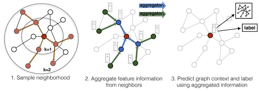
• Neighborhood aggregation methods, including graph convolutional methods, where both the node features
and the graph structure are used in the encoder network. Neighborhood aggregation methods use the graph
structure to propagate information across nodes and learn embeddings that encode structural properties about
the graph:
Z = ENC(W, X; ΘE ).
In what follows, we review recent methods for supervised and unsupervised graph embedding techniques using
G RAPH EDM and summarize the proposed taxonomy in Fig. 3.
4 Unsupervised Graph Embedding
We now give an overview of recent unsupervised graph embedding approaches using the taxonomy described in the
previous section. These methods map a graph, its nodes, and/or its edges, onto a continuous vector space, without using
task-specific labels for the graph or its nodes. Some of these methods optimize an objective to learn an embedding that
preserves the graph structure e.g. by learning to reconstruct some node-to-node similarity or dissimilarity matrix, such
as the adjacency matrix. Some of these methods apply a contrastive objective, e.g. contrasting close-by node-pairs
versus distant node-pairs [110]: nodes co-visited in short random walks should have a similarty score higher than
distant ones, or contrasting real graphs versus fake ones [135]: the mutual information between a graph and all of its
nodes, should be higher in real graphs than in fake graphs.
11Legend Laplacian MDS [Kruskal, 1964]
Section 4.1.1 IsoMAP [Tenenbaum, 2000]
Shallow embeddings LLE [Roweis, 2000]
LE [Belkin, 2002]
Auto-encoders
Non-Euclidean Poincaré [Nickel, 2017]
Section 4.1.2 Lorentz [Nickel, 2018]
Graph regularization ENC(ΘE ) Product [Gu, 2018]
Graph neural networks Matrix GF [Ahmed, 2013]
Factorization GraRep [Cao, 2015]
Section 4.1.3 HOPE [Ou, 2016]
X=I Skip-gram DeepWalk [Perozzi, 2014]
Section 4.1.4 node2vec [Grover, 2016]
WYS [Abu-el-haija, 2018]
LINE [Tang, 2015]
HARP [Chen, 2018]
Unsupervised
(α = 0)
ENC(W ; ΘE ) Autoencoders SDNE [Wang, 2016]
Section 4
Section 4.2 DNGR [Cao, 2016]
X 6= I ENC(W, X; ΘE ) Message passing GAE [Kipf, 2016]
Section 4.3 Graphite [Grover, 2019]
DGI [Veličković, 2019]
Graph
Embedding X=I ENC(ΘE ) Laplacian LP [Zhu, 2002]
Section 5.1 LS [Zhou, 2004]
Laplacian ManiReg [Belkin, 2006]
Section 5.2.1 SemiEmbed [Weston, 2008]
ENC(X; ΘE ) NGM [Bui, 2018]
Supervised
(α 6= 0) Skip-gram Planetoid [Yang, 2016]
Section 5 Section 5.2.2
Frameworks GNN [Scarselli, 2009]
Section 5.3.1 GGSNN [Li, 2015]
MPNN [Gilmer, 2017]
X 6= I GraphNets [Battaglia, 2016]
Spectrum-free ChebyNet [Defferrard, 2016]
Local Section 5.4.2 GCN [Kipf, 2016]
Message passing
Spatial SAGE [Hamilton, 2017]
Section 5.5 MoNet [Monti, 2017]
GAT [Veličković, 2018]
ENC(W, X; ΘE )
Non-Euclidean HGCN [Chami, 2019]
Section 5.6 HGNN [Liu, 2019]
Global filtering Spectrum-based SCNN [Bruna, 2014]
Section 5.4.1 [Henaff, 2015]
Figure 3: Taxonomy of graph representation learning methods. Based on what information is used in the encoder
network, we categorize graph embedding approaches into four categories: shallow embeddings, graph auto-encoders,
graph-based regularization and graph neural networks. Note that message passing methods can also be viewed as
spatial convolution, since messages are computed over local neighborhood in the graph domain. Reciprocally, spatial
convolutions can also be described using message passing frameworks.
12Z DEC(Z; ΘD ) W
c LG,REG W
Figure 4: Shallow embedding methods. The encoder is a simple embedding look-up and the graph structure is only
used in the loss function.
4.1 Shallow embedding methods
Shallow embedding methods are transductive graph embedding methods where the encoder function is a simple em-
bedding lookup. More concretely, each node vi ∈ V has a corresponding low-dimensional learnable embedding vector
Zi ∈ Rd and the shallow encoder function is simply:
Z = ENC(ΘE )
= ΘE ∈ R|V |×d .
Embeddings of nodes can be learned such that the structure of the data in the embedding space corresponds to the
underlying graph structure. At a high level, this is similar to dimensionality reduction methods such as PCA, except
that the input data might not have a linear structure. In particular, methods used for non-linear dimensionality reduction
often start by building a discrete graph from the data (to approximate the manifold) and can be applied to graph
embedding problems. Here, we analyze two major types of shallow graph embedding methods, namely distance-
based and outer product-based methods.
Distance-based methods These methods optimize embeddings such that points that are close in the graph (as mea-
sured by their graph distances for instance) stay as close as possible in the embedding space using a predefined distance
function. Formally, the decoder network computes pairwise distance for some distance function d2 (·, ·), which can
lead to Euclidean (Section 4.1.1) or non-Euclidean (Section 4.1.2) embeddings:
c = DEC(Z; ΘD )
W
with W
cij = d2 (Zi , Zj )
Outer product-based methods These methods on the other hand rely on pairwise dot-products to compute node
similarities and the decoder network can be written as:
c = DEC(Z; ΘD )
W
= ZZ > .
Embeddings are then learned by minimizing the graph regularization loss: LG,REG (W, W c ; Θ) = d1 (s(W ), W
c ). Note
that for distance-based methods, the function s(·) measures dissimilarity or distances between nodes (higher values
mean less similar pairs of nodes), while in outer-product methods, it measures some notion of similarity in the graph
(higher values mean more similar pairs).
4.1.1 Distance-based: Euclidean methods
Most distance-based methods optimize Euclidean embeddings by minimizing Euclidean distances between similar
nodes. Among these, we find linear embedding methods such as PCA or MDS, which learn low-dimensional linear
projection subspaces, or nonlinear methods such as Laplacian eigenmaps, IsoMAP and Local linear embedding. Note
that all these methods have originally been introduced for dimensionality reduction or visualization purposes, but can
easily be extended to the context of graph embedding.
Multi-Dimensional Scaling (MDS) [80] refers to a set of embedding techniques used to map objects to positions
while preserving the distances between these objects. In particular, metric MDS (mMDS) [40] minimizes the reg-
ularization loss in Eq. (1) with s(W ) set to some distance matrix measuring the dissimilarity between objects (e.g.
13Euclidean distance between points in a high-dimensional space):
P c 2 1/2
ij (s(W )ij − Wij )
d1 (s(W ), W
c) = P 2
ij s(W )ij
cij = d2 (Zi , Zj ) = ||Zi − Zj ||2 .
W
That is, mMDS finds an embedding configuration where distances in the low-dimensional embedding space are pre-
served by minimizing a residual sum of squares called the stress cost function. Note that if the dissimilarities are
computed from Euclidean distances of a higher-dimensional representation, then mMDS is equivalent to the PCA
dimensionality reduction method. Finally, there exist variants of this algorithm such as non-metric MDS, when the
dissimilarity matrix s(W ) is not a distance matrix, or classical MDS (cMDS) which can be solved in closed form
using a low-rank decomposition of the gram matrix.
Isometric Mapping (IsoMap) [129] is an algorithm for non-linear dimensionality reduction which estimates the
intrinsic geometry of a data lying on a manifold. This method is similar to MDS, except for a different choice of the
distance matrix. IsoMap approximates manifold distances (in contrast with straight-line Euclidean geodesics) by first
constructing a discrete neighborhood graph G, and then using the graph distances (length of shortest paths computed
using Dijkstra’s algorithm for example) to approximate the manifold geodesic distances:
s(W )ij = dG (vi , vj ).
IsoMAP then uses the cMDS algorithm to compute representations that preserve these graph geodesic distances.
Different from cMDS, IsoMAP works for distances that do not necessarily come from a Euclidean metric space (e.g.
data defined on a Riemannian manifold). It is however computationally expensive due to the computation of all pairs
of shortest path lengths in the neighborhood graph.
Locally Linear Embedding (LLE) [116] is another non-linear dimensionality reduction technique which was intro-
duced around the same time as IsoMap and improves over its computational complexity via sparse matrix operations.
Different from IsoMAP which preserves the global geometry of manifolds via geodesics, LLE is based on the local ge-
ometry of manifolds and relies on the assumptions that when locally viewed, manifolds are approximately linear. The
main idea behind LLE is to approximate each point using a linear combination of embeddings in its local neighborhood
(linear patches). These local neighborhoods are then compared globally to find the best non-linear embedding.
Laplacian Eigenmaps (LE) [14] is a non-linear dimensionality reduction methods that seeks to preserve local dis-
tances. Spectral properties of the graph Laplacian matrix capture important structural information about graphs. In
particular, eigenvectors of the graph Laplacian provide a basis for smooth functions defined on the graph vertices (the
“smoothest” function being the constant eigenvector corresponding to eigenvalue zero). LE is a non-linear dimension-
ality reduction technique which builds on this intuition. LE first constructs a graph from datapoints (e.g. k-NN graph
or ε-neighborhood graph) and then represents nodes in the graphs via the Laplacian’s eigenvectors corresponding to
smaller eigenvalues. The high-level intuition for LE is that points that are close on the manifold (or graph) will have
similar representations, due to the “smoothness” of Laplacian’s eigenvectors with small eigenvalues. Formally, LE
learns embeddings by solving the generalized eigenvector problem:
min Z >L Z
Z∈R|V |×d
subject to Z > DZ = I and Z > D1 = 0,
where the first constraint removes an arbitrary scaling factor in the embedding and the second one removes trivial
solutions corresponding to the constant eigenvector (with eigenvalue zero for connected graphs). Further, note that
Z > L Z = 21 ij Wij ||Zi − Zj ||22 and therefore the minimization objective can be equivalently written as a graph
P
regularization term using our notations:
X
d1 (W, W
c) = Wij W
cij
ij
cij = d2 (Zi , Zj ) = ||Zi − Zj ||22 .
W
14Therefore, LE learns embeddings such that the Euclidean distance in the embedding space is small for points that are
close on the manifold.
4.1.2 Distance-based: Non-Euclidean methods
The distance-based methods described so far assumed embeddings are learned in a Euclidean space. Graphs are
non-Euclidean discrete data structures, and several works proposed to learn graph embeddings into non-Euclidean
spaces instead of conventional Euclidean space. Examples of such spaces include the hyperbolic space, which has a
non-Euclidean geometry with a constant negative curvature and is well-suited to represent hierarchical data.
To give more intuition, the hyperbolic space can be thought of as continuous versions of trees, where geodesics
(generalization of shortest paths on manifolds) resemble shortest paths in discrete trees. Further, the volume of balls
grows exponentially with radius in hyperbolic space, similar to trees where the number of nodes within some distance
to the root grows exponentially. In contrast, this volume growth is only polynomial in Euclidean space and there-
fore, the hyperbolic space has more “room” to fit complex hierarchies and compress representations. In particular,
hyperbolic embeddings can embed trees with arbitrary low distortion in just two-dimensions [119] whereas this is
not possible in Euclidean space. This makes hyperbolic space a natural candidate to embed tree-like data and more
generally, hyperbolic geometry offers an exciting alternative to Euclidean geometry for graphs that exhibit hierarchical
structures, as it enables embeddings with much smaller distortion.
Before its use in machine learning applications, hyperbolic geometry has been extensively studied and used in
network science research. Kleinberg [77] proposed a greedy algorithm for geometric rooting, which maps nodes in
sensor networks to coordinates on a hyperbolic plane via spanning trees, and then performs greedy geographic routing.
Hyperbolic geometry has also been used to study the structural properties of complex networks (networks with non-
trivial topological features used to model real-world systems). Krioukov et al. [79] develop a geometric framework
to construct scale-free networks (a family of complex networks with power-law degree distributions), and conversely
show that any scale-free graph with some metric structure has an underlying hyperbolic geometry. Papadopoulos et al.
[106] introduce the Popularity-Similarity (PS) framework to model the evolution and growth of complex networks. In
this model, new nodes are likely to be connected to popular nodes (modelled by their radial coordinates in hyperbolic
space) as well as similar nodes (modelled by the angular coordinates). This framework has further been used to
map nodes in graphs to hyperbolic coordinates, by maximising the likelihood that the network is produced by the PS
model [107]. Further works extend non-linear dimensionality reduction techniques such as LLE [14] to efficiently
map graphs to hyperbolic coordinates [8, 100].
More recently, there has been interest in learning hyperbolic representations of hierarchical graphs or trees, via
gradient-based optimization. We review some of these machine learning-based algorithms next.
Poincaré embeddings Nickel and Kiela [101] learn embeddings of hierarchical graphs such as lexical databases (e.g.
WordNet) in the Poincaré model hyperbolic space. Using our notations, this approach learns hyperbolic embeddings
via the Poincaré distance function:
d2 (Zi , Zj ) = dPoincaré (Zi , Zj )
||Zi − Zj ||22
= arcosh 1 + 2 .
(1 − ||Zi ||22 )(1 − ||Zj ||22 )
Embeddings are then learned by minimizing distances between connected nodes while maximizing distances between
disconnected nodes:
e−Wij
X c X
c) = −
d1 (W, W Wij log P =− Wij log Softmaxk|Wik =0 (−W
cij ),
e − W
cik
ij k|Wik =0 ij
where the denominator is approximated using negative sampling. Note that since the hyperbolic space has a manifold
structure, embeddings need to be optimized using Riemannian optimization techniques [19] to ensure that they remain
on the manifold.
Other variants of these methods have been proposed. In particular, Nickel and Kiela [102] explore a different
model of hyperbolic space, namely the Lorentz model (also known as the hyperboloid model), and show that it provides
better numerical stability than the Poincaré model. Another line of work extends non-Euclidean embeddings to mixed-
curvature product spaces [63], which provide more flexibility for other types of graphs (e.g. ring of trees). Finally,
Chamberlain et al. [28] extend Poincaré embeddings to incorporate skip-gram losses using hyperbolic inner products.
154.1.3 Outer product-based: Matrix factorization methods
Matrix factorization approaches learn embeddings that lead to a low rank representation of some similarity matrix
s(W ), where s : R|V |×|V | → R|V |×|V | is a transformation of the weighted adjacency matrix, and many methods set
it to the identity, i.e. s(W ) = W . Other transformations include the Laplacian matrix or more complex similarities
derived from proximity measures such as the Katz Index, Common Neighbours or Adamic Adar. The decoder function
in matrix factorization methods is a simple outer product:
c = DEC(Z; ΘD ) = ZZ > .
W (3)
Matrix factorization methods learn embeddings by minimizing the regularization loss in Eq. (1) with:
LG,REG (W, W c ||2 .
c ; Θ) = ||s(W ) − W (4)
F
That is, d1 (·, ·) in Eq. (1) is the Frobenius norm between the reconstructed matrix and the target similarity matrix. By
minimizing the regularization loss, graph factorization methods learn low-rank representations that preserve structural
information as defined by the similarity matrix s(W ) and we now review important matrix factorization methods.
Graph factorization (GF) [6] learns a low-rank factorization for the adjacency matrix by minimizing graph regu-
larization loss in Eq. (1) using:
X
d1 (W, W
c) = (Wij − Wcij )2 .
(vi ,vj )∈E
Note that if A is the binary adjacency matrix, that is Aij = 1 iif (vi , vj ) ∈ E and Aij = 0 otherwise, then we can
express the graph regularization loss in terms of Frobenius norm:
LG,REG (W, W c )||2 ,
c ; Θ) = ||A · (W − W
F
where · is the element-wise matrix multiplication operator. Therefore, GF also learns a low-rank factorization of the
adjacency matrix W measured in Frobenuis norm. Note that the sum is only over existing edges in the graph, which
reduces the computational complexity of this method from O(|V |2 ) to O(|E|).
Graph representation with global structure information (GraRep) [26] The methods described so far are all
symmetric, that is, the similarity score between two nodes (vi , vj ) is the same a the score of (vj , vi ). This might be
a limiting assumption when working with directed graphs as some nodes can be strongly connected in one direction
and disconnected in the other direction. overcomes this limitation by learning two embeddings per node, a source
embedding Z s and a target embedding Z t , which capture asymmetric proximity in directed networks. GraRep learns
embeddings that preserve k-hop neighborhoods via powers of the adjacency and minimizes the graph regularization
loss with:
c (k) = Z (k),s Z (k),t >
W
c (k) ; Θ) = ||D−k W k − W
LG,REG (W, W c (k) ||2 ,
F
for each 1 ≤ k ≤ K. GraRep concatenates all representations to get source embeddings Z s = [Z (1),s | . . . |Z (K),s ] and
target embeddings Z t = [Z (1),t | . . . |Z (K),t ]. Finally, note that GraRep is not very scalable as the powers of D−1 W
might be dense matrices.
HOPE [104] Similar to GraRep, HOPE learns asymmetric embeddings but uses a different similarity measure. The
distance function in HOPE is simply the Frobenius norm and the similarity matrix is a high-order proximity matrix
(e.g. Adamic-Adar):
c = Z sZ t>
W
LG,REG (W, W c ||2F .
c ; Θ) = ||s(W ) − W
The similarity matrix in HOPE is computed with sparse matrices, making this method more efficient and scalable than
GraRep.
16You can also read