The Offense-Defense Balance and The Costs of Anarchy: When Welfare Improves Under Offensive Advantage

The Offense-Defense Balance and The Costs
of Anarchy: When Welfare Improves Under
Offensive Advantage
R. Daniel Bressler1, Robert F. Trager2, and Allan Dafoe3

 Abstract A large literature has argued that offensive advantage makes states worse off
 because it can induce a security dilemma, preemption, costly conflict, and arms races. In
 this paper, we challenge this prevailing wisdom. We argue that state welfare is u-shaped
 under increasing offensive advantage. We assess the effect of the offense-defense balance
 by considering a model where two states choose arms levels and decide whether to
 attack. High defensive advantage is first-best because attacking is difficult and the arms
 burdens required to deter attacks and maintain peace are low. High offensive advantage is
 comparatively worse because war is likely, but war tends to be smaller in scale, quicker,
 and less costly. Intermediate offensive advantage is worst because high arms burdens
 are required to deter attacks while wars, when they occur, are larger, longer, and more
 destructive. We discuss historical examples of this phenomenon from the Warring States
 periods in China and Japan, the Mongol invasions of the Middle East, the Imjin War, the
 Federalist papers, the Napoleonic Wars, the American Civil War, and the World Wars.
 A large literature has argued that offensive advantage makes states worse off because
 it can induce a security dilemma, preemption, costly conflict, and arms races. We argue
 instead that state welfare is u-shaped under increasing offensive advantage. We assess
 the offense-defense balance by considering a model where two states choose arms levels
 and decide whether to attack. High defensive advantage is first-best because attacking
 is difficult and the arms burdens required to deter attacks and maintain peace are low.
 High offensive advantage is comparatively worse because war is likely, but war tends to
 be smaller in scale, quicker, and less costly. Intermediate offensive advantage is worst
 because high arms burdens are required to deter attacks while wars, when they occur, are
 larger, longer, and more destructive. We discuss historical examples of this phenomenon
 including from the Warring States periods in China and Japan, the Federalist papers, and
 the World Wars.

 1. PhD Candidate, Columbia University School of International and Public Affairs. Correspondence to
rdb2148@columbia.edu
 2. Associate Professor, University of California Los Angeles
 3. Associate Professor and Director of the Centre for the Governance of AI, Future of Humanity Institute,
University of Oxford

Introduction
 Does greater offensive advantage necessarily lead to worse outcomes in the
anarchical international system? A large body of past literature has suggested that the
answer is yes. When offense is advantaged, wars are more likely4. Because attacks are
more likely to be successful, revisionist states are more likely to attack their rivals. In
addition, there are greater incentives for preemption, as states would rather attack than
defend in the event of war. Status quo states, who may have little interest in taking
their opponent’s territory, now have greater reason to fear other states’ armies and may
end up attacking out of fear. The security dilemma – when one state takes measures
to improve its own security, but in the process decreases the security of other states –
is exacerbated. A state may build up its military to protect itself against surrounding
states, but in circumstances in which offense is advantaged, other states are more likely
to view this as a threat to their own security. In short, situations in which offense is
advantaged are more dangerous and belligerent. Because war is costly and leads to
death and destruction, offensive advantage is comparatively dangerous and ruinous
relative to sanguine defensive advantage.
 In this paper, we challenge this prevailing wisdom. We argue that the relationship
between offensive advantage and outcomes in the anarchical international system is
more complex. Under certain conditions, we argue that increasing offensive advantage
can lead to better outcomes.
 We show this by producing a formal model of two single unitary actor states
coexisting under anarchy, and by providing a number of historical examples. Our
model builds on and extends James Fearon’s model from Cooperation, Conflict, and
the Costs of Anarchy.5 Fearon’s goal was to create a baseline model that characterizes
the strategic problems facing states interacting in international anarchy, and we found
his model useful as a springboard to explore the impact of the offense-defense balance
on welfare. Fearon’s analysis was focused on determining the conditions under which a
peace equilibrium could be supported, and on analyzing the attractiveness of outcomes
in peace equilibria. We extend Fearon’s analysis to model war equilibria in addition
to peace equilibria, and we show how state welfare (defined as the net present value of
state payoffs) changes in equilibrium under comparative statics in the offense-defense
balance parameter. We further extend Fearon’s analysis by exploring equilibria in
which states place some value on the present relative to future periods (i.e. they have a
discount rate bounded away from zero) and we use constrained optimization methods
to solve for a reduced-form solution to the model.
 We consider three successively elaborate iterations of this model. In each iteration
of the model, we establish propositions that continue to hold in subsequent model
iterations. In the first iteration, we consider a single-shot model with exogenous arms

 4. Jervis 1978; Van Evera 1998; Gilpin 1983; Glaser and Kaufmann 1998; Hart 1932; Lynn-Jones 1995;
Quester 2002.
 5. Fearon 2018.

 2

levels. War, when it occurs, is modeled in reduced-form and the costs of war are
exogenous. In the second iteration, we extend the single-shot model into an infinitely
repeated dynamic setting where arms are now chosen endogenously, but war continues
to be modeled in reduced form and war costs are exogenous. In the third iteration, we
extend the dynamic model so that war is modeled as a series of operations and war
costs are endogenous.
 We show that increasing the offense-defense balance from extreme defensive
advantage to extreme offensive advantage causes the game to switch from an equi-
librium in which peace is the only outcome to an equilibrium in which war is the
only outcome (proposition 1). We show that state welfare is strictly decreasing in
offensive advantage in peace equilibria (proposition 2). This is because as offense
becomes increasingly advantaged, states must allocate a greater portion of their scarce
resources to arms so as to deter the other side from attacking. Because arms cannot
be consumed or invested, arms spending reduces welfare. These results are largely in
line with past arguments around the offense-defense balance.
 When we consider state welfare in war equilibria, however, we find results that
depart from arguments made in prior work. We find that increasing offensive advantage
increases welfare in war equilibria for two main reasons: (1) Wars tend to be less total6
under higher levels of offensive advantage, and (2) Wars tend to be more decisive,
shorter, and less costly under higher levels of offensive advantage.
 On point (1), we find that once offense is advantaged over the defense, further
increases in offensive advantage tend to make wars less total by reducing equilibrium
arms spending in war as long as states place some value on the present relative to the
future (proposition 3). This is because the returns to arming decrease under increasing
offensive advantage. The intuition for this is straightforward: as offense becomes
increasingly advantaged, having a marginally larger or better military becomes less
important compared to being the attacker in a war. Likewise, if defense is quite
advantaged in a war, then a marginally larger or better military is also less important
compared to being the defender. Arms provide the greatest return on investment
(where returns are measured as an increased probability of winning the war) when there
is offense-defense neutrality, i.e. for given force levels, a state has the same probability
of winning regardless of whether they are attacking or defending. Therefore, arms
investments are the highest and wars are the most total under offense-defense neutrality.
As the offense-defense balance shifts away from offense-defense neutrality in either
the offensive or defensive direction, arms investments decrease, and wars become less
total, which increases the welfare of the states involved.
 We demonstrate point (2) by modelling war as a series of operations. We find that
under higher levels of offensive advantage, there are fewer expected operations because
wars are more likely to end decisively instead of bogging down into a stalemate and

 6. By less total, we mean that the war is fought with a lower proportion of the state’s resources. In the
context of our model, a war is less total when the equilibrium arms spending is lower.

 3

further operations. Therefore, wars tend to be shorter and less costly under higher
levels of offensive advantage. This is consistent with arguments made in a large
body of past literature that under higher levels of offensive advantage wars tend to be
“shorter,”7 “quick and decisive,”8 and “relatively quick, bloodless, and decisive.”9
 In summary, our analysis suggests that starting from extreme defensive advantage,
greater offensive advantage has adverse effects: it creates more conditions under
which war occurs, and under peace, it makes states worse off through the higher arms
spending required to maintain deterrence. In war equilibria, however, marginally
increasing offensive advantage will tend to make states better off for the two reasons
stated above. This gives state welfare under offensive advantage a general u-shape (a
phenomenon we abbreviate WUO for Welfare is U-shaped under Offensive advantage).
Importantly, this suggests that large increases in offensive advantage can cause an
absolute increase in state welfare by switching from a costly peace equilibrium
burdened by high arms levels to a decisive war equilibrium. (proposition 5).
 In short, war is inefficient, but so is a costly peace. A large exogenous increase
in offensive advantage due to some change in military technology, for instance, can
provide the spark for states to engage in a decisive war that results in state consolidation
with no future costs of anarchy because there is no more anarchy. This outcome can
be welfare-improving over a continued costly peace.10
 Historical examples of the phenomena we describe can be drawn from the histories
of Japan and China, mentioned briefly here and discussed in more detail in the main
body of the paper. Japan endured a bloody period of warring states (the Sengoku Jidai,
roughly 1467-1600) in which the country dissolved into hundreds of independent
states run by warlords (daimyōs). The prevailing military organization and technology
available at the time made it difficult for warlords to conquer and hold large swaths of
territory, so the country remained in bloody civil war for over a hundred years.This
state of affairs ended only at the end of the 16th century when the three great unifiers
of Japan – Oda Nabunaga, Toyotomi Hideyoshi, and ultimately Tokugawa Ieyasu were
able to revolutionize military organization and utilize new technologies so that it was
possible to conquer and hold large swaths of territory and to ultimately consolidate
Japan into a single state, ending the state of anarchy and ushering in the peaceful
and prosperous Edo period (1600-1868). Similarly, China endured a bloody period
of warring states from 475-221 BC until it was unified by Emperor Qin Shi Huang.
Similar to the Japanese Warring States period, the end of this period was marked
by increased offensive advantage due to innovations in military organization and

 7. Fearon 1995.
 8. Glaser and Kaufmann 1998.
 9. Jervis 1978.
 10. See (Coe 2011) and (Kydd 2015) chapter 7 for analysis of the costly peace and costly deterrence
explanations for war as well as (Powell 1993) and (Hwang 2012). (Fearon 2018) footnote 15 shows that
Immanuel Kant also identified and described this explanation for war in 1795 (Kant 1983). Our analysis
shows that a change in the offense-defense balance towards offensive advantage can be a mechanism by
which the equilibrium flips from costly peace to a decisive war, which can be welfare improving.

 4

technology, in particular, siege technology. At the end of this period, Qin Shi Huang
was able to put an end to the warring states period by conquering all of China in a
rapid campaign that lasted only 9 years. Historically, China was most prosperous
when a single dynasty ruled the country, even though the costs of conquering China
were very high in both material and human terms.
 Finally, we emphasize that these results should be interpreted with caution. States
are best off when defense is highly advantaged and peace can be maintained. Moreover,
caution is further required because governments and military leaders in the past have
misjudged the offense-defense balance, often in the direction of overestimating the
viability of offense.11 Much of the death and suffering from war historically has
resulted from wars that were expected to be swift and decisive but ended up being
years-long attrition contests. These include the 1592 Japanese invasion of Korea,
the 1914 Austro-Hungarian invasion of Serbia, the 1937 Japanese invasion of China,
the 1941 German invasion of the Soviet Union, the 1950 North Korean invasion of
South Korea, and the 1980 Iraqi invasion of Iran. In addition, consolidation through
federation is superior to consolidation through war because it achieves the benefit
of removing the costs of anarchy while avoiding the cost of war (see conclusion for
further discussion). However, our analysis suggests that if consolidation through
federation is not possible, then consolidation through war may be welfare improving
over a continued costly and risky peace.

Offense-Defense Balance in a Single Stage Model
 We begin by considering a simple single stage version of our model where arming
and war costs are exogenous. The players, payoffs, and propositions introduced in this
single stage model will remain the same in the two further more elaborate iterations
of the model in the following sections.12
 There are two state actors with resource endowments normalized to 1. Players
are endowed with arms levels ∈ [0, 1], which are subtracted from their resource
endowments. Arms do not provide utility, but are useful in winning a possible
war against the other state. Player payoffs are measured in units of their resource
endowments, and we make the standard simplifying assumption that player utility is
synonymous with their payoffs. Players value international issues, ∈ (0, 1). In the
absence of war, is divided equally between the states.13 Players also place some

 11. Hart 1932; Snyder 1984; Van Evera 1984.
 12. The payoffs introduced in this section align with the payoffs in Fearon’s original model. However,
Fearon’s model was focused on determining conditions under which the peaceful equilibrium could be
maintained by arming up enough to deter an opponent from attacking. We begin to extend Fearon’s model
in this section by analyzing war equilibria, both (1) when one player attacks and the other defends, and (2)
when both players simultaneously attack each other.
 13. In this simplified iteration of the model, we make the assumption that is divided evenly in peace
equilibria, but in following model iterations, we will discuss the role of bargaining.

 5

value on ruling the other state’s territory in the event that they win the war, ∈ [0, 1].
 Players simultaneously choose whether to attack or not attack. There is only peace
when neither side attacks. Although actions take place in a single stage, payoffs are
assumed to last in perpetuity14 and are discounted by the factor ∈ [0, 1). War is
treated as a costly lottery where the loser is eliminated and gets a payoff of 0 henceforth.
The winner gets full control of issues and the other sides’ endowment henceforth.
The winner continues to receive their resource endowment without further need for
arms spending because the other side has been eliminated in the war. The winner must
also pay the costs of war ≥ 0. We assume that these costs are paid in perpetuity for
convenience.15 We make the simplifying assumption that the two states have identical
preferences, resources, and arms levels.
 In summary, the benefit from winning a war16 is given by:

 − + (1 + ) 
 =
 1− 1− 
 We simplify the notation by defining = − + (1 + ) as the single-period
benefit of winning the war, which is then converted into a perpetuity by dividing by
1 − .
 The probability of victory for state i in a war with state j is determined by the
contest success function (CSF) ( , ; ).17 The probability of victory for state i
attacking state j is given by the CSF ( , ; ), the probability of victory for state
i defending against state j is determined by the CSF ( , ; ), and the probability
of victory for state i when state i and state j simultaneously attack is determined by
the CSF ( , ; ). ≥ 0 is the offense-defense parameter. A larger m implies
greater offensive advantage, i.e. for a fixed level of arms levels, the greater the
probability that the attacker has of winning the war. A formal treatment of CSFs and
their relationship to the offense-defense balance is given in the appendix.18

 14. We make this assumption so that we can use the payoffs from this section in all subsequent sections
when the model is extended into an infinitely repeated setting.
 15. Following Fearon, although the costs of war can theoretically enter the model in a variety of ways,
this ensures that the cost term is relevant when we consider the case when → 1.
 16. Note that this is the payoff from the period after the war onward.
 17. In this single-shot model, arms levels are exogenous and identical between the two states, so the CSF
is determined only by the offense-defense balance. When we embed this single-shot model in a dynamic
setting with endogenous arms levels in the following section, the distinction between and will become
relevant.
 18. For brevity, we will sometimes drop the state superscript and all or some of the variables of the
function. We represent the CSF simply as , or when we want to emphasize whether a state
is attacking, defending, or if there is simultaneous attack. We represent the CSF simply as ( ) when
we want to present a general CSF without specifying whether the state is attacking or defending, but
emphasizing that the CSF is a function of the offense-defense balance. Regardless of the notation, the CSF
always represents some state’s probability of victory in a war with another state, is defined either in the
context of an attack, a defense, or a simultaneous attack, and is always a function of the states’ arms levels
and the offense-defense balance.

 6

The general expected payoff from war (not specifying whether the player is
attacking, being attacked, or if there is simultaneous attack) is given by:
 
 ( ) = 1 − + ( ) ∗
 1− 
 The expected payoff from peace is:

 1 − + /2
 ( ) =
 1− 
 Under peace, we assume that both players continue to spend on arms in perpetuity.
A summary of this single shot model in strategic form is shown in figure 1.

 FIGURE 1. The Single Stage Model in Strategic Form

Defining The Offense-Defense Balance Parameter
 So what exactly do we mean by the offense-defense balance in this model? Past
literature has used a variety of definitions for the offense defense balance including
the ease of territorial conquest,19 the characteristics of armaments that favor either
attackers or defenders,20 the relative resources needed by the offense in order to
overcome the defense,21 and the ratio of the cost of the forces that the attacker
requires to take territory to the cost of defender’s forces.22 There are also differences

 19. Van Evera 1998.
 20. Hart 1932.
 21. Gilpin 1983.
 22. Glaser and Kaufmann 1998; Lynn-Jones 1995.

 7

in the factors that past scholars have argued affect the offense-defense balance. Is
the offense-defense balance only determined by military technology, or is it also
determined by doctrine and geographic factors? Is the offense-defense balance a
system-wide variable that applies to any conflict that takes place at a certain point in
time, or does it vary at a given point in time depending on situation-specific factors?
Does the offense-defense balance apply to specific military campaigns, to whole wars,
or to both? Past analyses have answered these questions in different ways.23
 In our model, the offense-defense balance is defined in the context of a CSF
that determines the probability that one side wins a contest versus another side.24
Because we are working with a dyadic model, we are considering a dyad-specific
offense-defense balance, and we do not consider potential balancing or bandwagoning
effects.The CSF is a function of each side’s arms levels and the offense-defense
balance. The offense-defense balance is a variable that represents all of the factors
outside of arms levels that increase an attacker’s chance of success relative to the
defender or vice versa.
 This implies that we take a broad interpretation of the offense-defense balance:
military technology, doctrine, geography, nationalism, psychology, and other factors
can all in principle affect the offense-defense balance parameter, provided they increase
or decrease an attacker’s chance of success against a defender for given arms levels.
 To illustrate: the development of military technology25 such as better siege
weapons can shift the offense-defense balance in favor of the offense because they
make fortifications a less effective means of protecting territory.26 For a given set of
technologies, changes in military doctrine can favor either the offense or defense. For
instance, Nazi Germany’s organization of independent Panzer divisions that could
race ahead of the infantry to encircle enemies in large kesselschlacht (cauldron battles,
or battles of encirclement) shifted the balance in favor of attackers relative to doctrines
that placed tanks in infantry divisions so that they moved at the speed of the infantry.
Defense-in-depth tactics – where defense is constructed in multiple layers that all must
be breached instead of a single layer – such as those employed by the Germans in the

 23. (Levy 1984) primarily considered military technologies and doctrine. (Mearsheimer 2001) identified
the “stopping power of water” as a critical geographic factor consistent across time that favors defenders
that have to be invaded by sea, although he did not define this concept explicitly within the context of
offense-defense balance. (Glaser and Kaufmann 1998) argued that their definition of offense-defense
balance should apply to whole wars, and not specific battles. (Biddle 2001) argued that offense-defense
balance applies at the operational level and the best defensive strategies typically involve “defense in depth”
in which the defender may give ground to the attacker, but have forces in reserve that can counterattack.
(Lieber 2000) argues that focusing the offense-defense balance concept on technology is more useful than
considering a broader range of factors.
 24. We use the offense-defense balance parameter in the same way as (Fearon 2018). See equations (5),
(6), and (7) and subsequent discussion below.
 25. A good deal of recent literature has explored how advances in cyberwarfare affect the offense-defense
balance, including (Garfinkel and Dafoe 2019; Gartzke and Lindsay 2015; Slayton 2017; Lieber 2014).
 26. See our later discussion of the Japanese and Chinese Warring States Periods for more detail on the
effect of siege weapons.

 8

1917 Second Battle of the Aisne and by the Soviets in the 1943 Battle of Kursk, can
shift the balance in favor of defenders.27
 Geographic factors that make it harder to project force when invading, such as
large bodies of water, tend to shift the balance in favor of defenders.28 Nationalism can
provide defensive advantage when armies feel that they are protecting their homeland
against invaders, e.g. for the French in the 1792 campaigns of the War of the First
Coalition as captured in the song "Chant de Guerre pour l’Armée du Rhin," which has
since become the French National anthem.
 Separate from nationalism, psychological factors can also affect the offense-defense
balance. The phenomenon of loss aversion predicted by prospect theory may cause
defenders to fight harder to defend ground that they believe is theirs relative to attackers
that believe that they are capturing new territory.29 When defenders believe that they
will be massacred by attackers, they are more likely to fight to the death instead of
surrendering, shifting the balance towards the defense.30 Historical examples of this
include Nazi Germany’s Commissar Order to summarily execute Political Commissars
when they invaded the Soviet Union in 1941 and Hulagu Khan’s threats against the
Mamluk Sultanate that strengthened the resolve of the Mamluks in their victory over
the Mongols at Ain Jalut in 1260.31

 27. These examples bring up the important historical consideration that one side may figure out how to
optimally employ technology in their doctrine before the other side, as discussed in (Fearon 1995). For
instance, the Germans in the 1940 Battle of France placed nearly all of their armor in 10 independent
Panzer divisions, such as Erwin Rommel’s famed "Ghost Division," that could take advantage of the tank’s
speed in attack whereas the French integrated more of their tanks in with their infantry units (Zaloga 2014).
For this reason, we might expect that a German attack on France would favor the offense more than a
French attack on Germany. Our model makes the simplifying assumption that both sides are symmetric
in their resources, preferences, and they share a common offense-defense balance. One could relax this
assumption so that there is a different offense-defense balance depending on who is in attack. In this case,
the mechanisms identified in this paper that contribute towards WUO – (1) Higher arming required to
deter adversaries when they enjoy higher offensive advantages (2) Lower returns to arms under increasing
offensive advantage and (3) More decisive and less costly wars – would still hold, although this would
significantly complicate the analysis.
 28. See (Mearsheimer 2001) for a discussion of the stopping power of water.
 29. See (Levy 1997) and (Levy 2000) for discussion.
 30. Some of these factors affecting the offense-defense balance may arise endogenously as a strategic
response. However, our model treats the offense-defense balance as exogenous for analytical tractability
and to understand how outcomes change when factors external to the model cause the offense-defense
balance to change. See the conclusion for a discussion of how the balance can change endogenously and
suggestions for future work.
 31. In 1260, Hulagu Khan sent a letter to Sultan Qutuz of the Mamluk Sultanate reading: "Resist and
you will suffer the most terrible catastrophes. We will shatter your mosques and reveal the weakness of
your God, and then we will kill your children and your old men together" (Tschanz 2007). Similar threats
were commonly used by the Mongols as part of a psychological warfare strategy to coerce enemies into
capitulating without a fight. To make these threats credible, they would spare states that gave into the
demands and they would crush those that opposed them with extreme brutality. Just two years earlier,
Hulagu Khan had sent a similar letter to the Abbasid Caliphate. When they defied him, he destroyed
Baghdad in 1258 in one of the most brutal atrocities in history; estimates of the number of deaths range from
the hundreds of thousands to the millions (Iskandar et al. 2001; Wink 1991). Such tools of psychological

 9

The factors relevant to understanding the offense-defense balance varies signifi-
cantly across dyads and across time. For example, geographic factors can be critical.
Over centuries, the offense-defense balance in the France-Germany dyad favored the
offense more-so than the Britain-France dyad, due to the English Channel and the
stopping power of water. In the Napoleonic Wars, Napoleon was able to facilitate
swift movement of his armies deep in enemy territory by having them live off of the
land instead of burdening them with large supply columns. When fighting Austria and
Prussia in agriculturally-dense central Europe, this strategy worked well. His ability
to move his armies swiftly allowed him to conduct rapid battles of encirclement,32
and allowed him to quickly position his army near his enemy’s capitals to force them
into decisive battles.33 Russia, in contrast, was poorer and less agriculturally-dense.
Therefore, Napoleon could not employ the living off of the land strategy there. In
his 1812 invasion of Russia, Napoleon had to provide for a vast network of supply
columns that slowed his movement, making it more difficult to force the Russians into
a single decisive battle.34 Together, these factors imply that the France-Russia dyad
during the Napoleonic wars was more defense-dominant than the France-Austria or
France-Prussia dyad.
 In addition, it is important to clarify what we mean by "attacker," and "defender."
In our model, the attacker is the side that strikes first in a war. The examples given
at the end of the introduction all capture what we mean by attacker: Japan in their
1592 invasion of Korea, Austria-Hungary in their 1914 invasion of Serbia, Germany
in their 1941 invasion of the Soviet Union, North Korea in their 1950 invasion of
South Korea, and Iraq in their 1980 invasion of Iran. The attacker in our model is
not necessarily the country that declares war first; it is the country that attacks first.
For instance, in the War of the Fourth Coalition in 1806, Prussia declared War on
France first, but under our definition, France was the attacker and Prussia was the
defender because Napoleon quickly responded to Prussia’s declaration of war by
invading Prussian territory. Between 1939-1941, Nazi Germany was a prolific attacker
under our definition, launching large-scale invasions of Poland, Denmark, Norway, the
Netherlands, France, Yugoslavia, Greece, and the Soviet Union. A historical example

warfare either amplify the offense-defense balance towards more extreme offensive advantage or more
extreme defensive advantage. When they work, they cause extreme offensive advantage because the
defender gives up without a fight. When the defender does not capitulate, however, they contribute towards
stronger defensive advantage because the defender either wins or faces certain death. In the case of the
Mamluk Sultanate, Hulagu Khan’s threats backfired and ended up favoring the defense: before the battle,
Sultan Qutuz gave a speech to his troops stating that there was no alternative to winning except a horrible
death for themselves and their families, as the Mongols had made clear in their threats and with their actions
in Baghdad. The speech was effective in inspiring the men to fight exceptionally hard in close-quarter
fighting at the Battle of Ain Jalut, annihilating the Mongol force in a decisive victory that some observers
claimed saved Islam from the Mongol hordes (Amitai-Preiss 2004)
 32. Such as at Ulm (1805)
 33. Such as Austerlitz (1805), Jena–Auerstedt (1806), and Wagram (1809).
 34. In addition, the vast amount of territory between the Neman River and Moscow allowed the Russians
to trade space for time much more easily than Austria and Prussia.

 10

that captures what we mean by simultaneous attack are the attacks carried out by
Germany (the Shlieffen Plan) and France (Plan XVII) in 1914. These attacks were
executed at roughly the same time to initiate the Western Front theater of operations
in World War I.35
 In the first two iterations of our model, we consider the offense-defense balance at
the strategic level (i.e. the level of the outcome of the war). In the third iteration of
our model, we consider war as a series of operations, and the offense-defense balance
applies at the operational level. We show in that section that offensive advantage at
the operational level also implies offensive advantage at the strategic level.

Results from the Single Stage Model
 Whether a peace equilibrium can be supported in the single stage model shown in
Figure 1 depends on the best response to a non-attacking defender. We define this
condition as the static war constraint.36

 1 − + /2 
 ≥ 1 − + ( ) (1)
 (1 − ) (1 − )
 Depending on the offense-defense balance and the static war constraint, the game
can take one of four different structures. These game structures determine three
different strategic contexts that have been much discussed in the international relations
literature, Offensive War (scenario 1), Security Dilemma (scenario 3), and Stable
Deterrence (scenario 4), as well as an outcome that is less discussed in international
relations: Rope-A-Dope (scenario 2). Figure 2 shows these four outcomes with their
pure strategy Nash equilibria represented with the label N.E. Delineation into columns
indicates whether a predatory attack is attractive or not, i.e. whether the static war
constraint is satisfied.38 Delineation into rows determines whether offense or defense
is advantaged.

 35. Germany launched a large-scale attack through Belgium into Northern France beginning on August
5, 1914 and France launched a large-scale attack into Alsace-Lorraine under their Plan XVII beginning
on August 7, 1914. Both sides believed that the balance favored the offense, and they thus both believed
it was a best-response to attack, resulting in a simultaneous attack equilibrium. Ultimately, the German
attack was more successful (which fits with our coin flip simultaneous attack CSF, see equation 7 below
for more detail), as the French attack was pushed back immediately at the Battle of Mulhouse while the
German attack nearly reached Paris before being pushed back at the First Battle of the Marne. From there,
the Germans subsequently retreated and dug into defensible positions along the Aisne river, initiating the
Race to the Sea and setting off the Western Front lines that would remain fairly static for most of the war.
 36. We call this the static war constraint to differentiate it from the dynamic war constraint where arms
levels are chosen in a multi-stage process in the next section. If the static war constraint holds, then
remaining at peace is more attractive than a predatory attack,37 and a peace equilibrium can be supported.
If the war constraint does not hold, then a predatory attack is more attractive than remaining at peace.
Formally, the static war constraint holds when:
 38. For simplicity, we assume that "the tie goes to peace." If the war constraint holds with equality, then
we assume that (no attack) is the only best response to (no attack), i.e. a predatory attack is not attractive.

 11

FIGURE 2. The Four Scenarios of the Single Stage Game

 When offense is advantaged (top row), states do not want to get stuck defending
in a war. Therefore, a state’s best response is to attack when they expect the other
side to attack. There is always an equilibrium where both sides simultaneously attack
regardless of whether the static war constraint is satisfied.
 When defense is advantaged (bottom row), states prefer to being the defender in the
event of war. Therefore, when states expect the other side to attack, their best response
it to defend. There is never a pure strategy equilibrium where states simultaneously
attack regardless of whether the static war constraint is satisfied.
 When the war constraint is not satisfied, (left column) all pure strategy Nash
equilibria involve war because the best response to a non-attacking state is to attack.
 When the war constraint is satisfied (right column), then at least one of the pure
strategy Nash equilibria involves peace because the best response to a non-attacking
state is no attack.
 Scenario 1 – when offense is advantaged and the static war constraint is not
satisfied – yields Offensive War. In this scenario, countries seek hegemony through
conquest because attack is the dominant strategy for both players and war is the
only equilibrium outcome. A historical example that captures this equilibrium is the
simultaneous attack by both France and Germany to initiate the Western Front theater
of operations in World War I described earlier. Although they were mistaken, both
sides believed that the balance favored the offense, and they thus both believed it was
a best-response to attack, resulting in a simultaneous attack equilibrium.
 Scenario 3 – when offense is advantaged and war is relatively less attractive – yields

 12

dynamics similar to the Security Dilemma. In this scenario, war is not preferable for
either party and we might expect states to be able to cooperate to avoid war. However,
if the sides believes that the other will attack, the game can end up in the Pareto
dominated pure strategy Nash equilibrium of simultaneous attack because a country’s
best response to an attacker is to also attack to avoid being the disadvantaged defender
in war.39 This scenario is similar to the “doubly dangerous" scenario described by
Jervis (1978) in his discussion of the Security Dilemma.40 This game has the structure
of a stag hunt: a coordination game with multiple pure strategy Nash equilibria of
simultaneous attack and peace.

 Scenario 4 – when defense is advantaged and war is relatively less attractive –
results in Stable Deterrence. No attack is the dominant strategy for both countries.
This is the only scenario in which war is not an equilibrium. Even though attacking is
an option available to states and there is no global government to enforce contracts
between them, it is a never best response because war is relatively unattractive
compared to peace ( is sufficiently low), and defensive advantage implies that states
are better off letting a state attack them if they believe another state is planning to
attack.

 Scenario 2 – when defense is advantaged, but war is relatively more attractive –
yields hypotheses that are less discussed in international relations. We call scenario 2
the “Rope-a-Dope" scenario. The best outcome for a state in this scenario is to be
attacked by their opponent so that they can leverage defensive advantage and have the
best chance of winning the war. A state’s best response to a non-attacking opponent
is to attack despite defensive advantage due to the unattractiveness of peace relative
to a decisive war. This gives the game an anti-coordination structure that resembles
the game of chicken.41 This requires a predatory attack to be preferred to peace even
though the offense-defense balance favors defenders, which implies that the benefit
from winning a war is quite high (high ). Historically, this logic seems to undergird

 39. We get this result even though this is a game of complete information, and therefore there is no
uncertainty about players’ types and their intentions, although the model could be extended to include
incomplete information.
 40. Jervis 1978.
 41. This scenario is named after the strategy employed by Muhammad Ali in his famed “Rumble in the
Jungle" fight with George Foreman in 1974. Ali’s strategy was to allow the hard-punching Foreman to take
the offensive. Ali was good defensively and he could use the ropes of the boxing ring to aid in absorbing
Foreman’s blows. This had the effect of causing Foreman to tire, allowing Ali to counterattack late in the
fight and to knock out Foreman. The strategy is called “Rope-A-Dope" because Ali appeared to be a “dope"
on the ropes who was taking a beating from Foreman, but in actuality he was pursuing a defensive strategy
to let Foreman tire himself out on the offensive so that he could counterattack later and ultimately win the
fight (Erenberg 2019).

 13

decisionmaking on multiple occasions when defense was advantaged in wartime.4243
 In addition to the four scenarios shown in Figure 2, there is another possible
scenario: the cost of a war may be so high that peace is preferable to a predatory attack
that succeeds with 100% certainty. In this case, attacking is a never best response
irrespective of the offense-defense balance. We call this the Pyrrhic Victory Condition.

 Definition 1: Pyrrhic Victory Condition: If war costs are sufficiently high such
that peace is preferred to a predatory attack that succeeds with 100% certainty, then
attacking is a never best response and the Pyrrhic Victory condition holds.

 Formally, the Pyrrhic victory condition holds in the single stage model when the
following inequality holds:

 42. On the Western Front in World War I. In 1915, the Germans withstood a series of Entente offensives
against their entrenched positions that all resulted in little ground taken despite local Entente force superiority
and much higher casualties for the attackers relative to the defenders. These include winter offensives at the
First Battle of Champagne and the First Battle of Artois (December 1914-January 1915), a spring offensive
at the Second Battle of Artois (May-June 1915), and Autumn offensives at the Third Battle of Artois and
the Second Battle of Champagne (September-November 1915). Because of their futility, historian A.J.P.
Taylor describes the Entente offensives of 1915 as having "no meaning except as names on a war memorial"
(Taylor 1963). These results convinced German General Staff Chief Erich von Falkenhayn that the key to
victory on the Western Front was to goad the French into attacking German defensive positions so that
German artillery and machine guns could cut down attacking troops in open ground and “bleed white" the
French army. This was the strategy that informed the planning for the 1916 Battle of Verdun. Falkenhahyn’s
experience in the Second Battle of Champagne in particular informed his planning for Verdun. In this battle,
the French failed to break through German defenses despite three to one local superiority in manpower
and artillery. French attacks on German defensive positions led to enormous casualties for the French
relative to the Germans, which Falkenhayn believed to be three to one, though subsequent scholarship has
estimated the ratios at between two to one and three to two (Foley 2005; Sondhaus 2011). Falkenhayn
planned a limited offensive to threaten the culturally significant city of Verdun while securing important
high-ground around the city. From there, the German artillery could decimate French counterattacks.
Falkenhayn expected that five Frenchmen would be taken out of action for every two Germans, (Watson
2014) which would force the French into a manpower shortage that would knock them out of the war. In
reality, while the initial German advance was successful, many of the advancing German troops overran the
limited objectives set by Falkenhayn to weaker positions, and they failed to capture some of the important
strategic high ground, which made them vulnerable to French artillery barrages. The result was an almost
year-long stalemate with a similar numbers of casualties on both sides that numbered over 700,000 men
(Philpott 2015).
 43. Arguably a similar logic undergirded some British thinking around Operation Sea Lion, the planned
German invasion of the United Kingdom in 1940. Winston Churchill knew that invasions by sea tend to
especially favor defenders – a lesson he learned from his role in planning the failed Gallipoli landings in
1915 (Carlyon 2002; Moorehead 2015) – an advantage further magnified by the UK’s especially powerful
Royal Navy. Although the Germans called off the planned invasion, Churchill said of the plan: “Had the
Germans possessed in 1940 well trained [and equipped] amphibious forces their task would still have been
a forlorn hope in the face of our sea and air power... there were indeed some who ... for the sake of the
effect the total defeat of his expedition would have on the general war, were quite content to see him try"
(Churchill 1987)

 14

1 − + /2 − + (1 + )
 > 1− +
 1− 1− 
 This simplifies to:
 
 > + ( + ) (2)
 2
 If the Pyrrhic Victory condition holds, then (no attack, no attack) is the only Nash
equilibrium irrespective of the offense-defense balance.44 In practice, the Pyrrhic
victory condition could result from the introduction of nuclear weapons or devastating
conventional weapons that impose high costs on the victor.45 This illustrates how
factors that increase the cost of war, such as nuclear weapons, can deter war separately
from their affect on the offense-defense balance.46
 With the exception of the offense-defense balance, all of the variables affect the
game structure by affecting the attractiveness of war relative to peace, which tightens
or loosens the static war constraint. Increasing greed for the other side’s territory
(higher ) and decreasing the costs of war (lower ) make war more attractive (higher
 ), which tightens the static war constraint. Higher arms levels (higher ) also make
war more attractive because arms are only needed in the single period of the decisive
war and not needed after hegemony has been obtained whereas in peace, arms must
be spent in perpetuity.
 The effect of the offense-defense balance is more complicated than any other
variable in the model because it effects the game both continuously and categorically,
whereas the other variables (e.g. , , and ) affect the game only continuously.
The offense-defense balance affects outcomes continuously because it changes the
attractiveness of war for attackers relative to defenders. The more offense is advantaged
(higher ), the higher the expected payoff from war for attackers47 and the lower the
expected payoff from war for defenders48 regardless of whether < 1 or > 1. The
result is that higher offensive advantage makes a predatory attack more attractive and
tends the game towards war equilibria and away from peace equilibria, similar to more

 44. If defense is advantaged and the Pyrrhic Victory condition holds, then the game structure is Stable
Deterrence. However, there are Stable Deterrence scenarios where the Pyrrhic Victory condition does not
hold: i.e. scenarios where a predatory attack is unattractive given the current probability of victory, but a
predatory would be attractive if victory could be guaranteed.
 45. Assuming that two states have nuclear weapons and possess a credible second-strike capability.
Nuclear weapons could contribute towards extreme offensive advantage if states can quickly destroy all of
the enemy’s forces through a preemptive counter-force strike. If both states possess a credible second-strike
deterrent, however, then there is mutually assured destruction and such an attack is not possible without
receiving a retaliatory strike that imposes enormous costs on the attacker and leaves both sides’ forces
depleted.
 46. Although the use of nuclear weapons in the event of war would have to be credible for this to hold.
 
 ∗ 1−
 47. Formally 
 
 >0
 ∗ 1− 
 48. Formally 

greed for the other side’s territory (higher ), lower costs of war (lower ), and higher
arms levels (higher ).
 The difference between defensive advantage ( < 1) and offensive advantage
( > 1) changes the structure of the game categorically from scenario 2 (Rope-A-
Dope) to scenario 1 (Offensive War) when a predatory attack is attractive. Thus, as
long as a predatory attack was already attractive before the discrete jump, switching
from defensive advantage to offensive advantage is arguably less consequential because
the game switches from one war pure strategy equilibrium (where one side attacks and
one side defends in scenario 2) to another war pure strategy equilibrium (simultaneous
attack in scenario 1). However, if a predatory attack is unattractive both before and
after the discrete jump from defensive advantage to offensive advantage, then the
structure of the game switches from scenario 4 (Stable Deterrence) to scenario 3
(Security Dilemma).
 In short, the net effect of increased offensive advantage in this one-shot model
with exogenous arms, in both its continuous and discrete effects, is to tend the game
structure away from peace equilibria and towards war equilibria. Insofar as war is
costly and leads to death and destruction, the sanguine defense-advantaged world
is preferable to the offense-advantaged world as past scholars have argued. We
summarize this result in the following proposition:

 Proposition 1: In the one-shot model with exogenous arms levels and with suffi-
ciently low war cost ( ) such that that the Pyrrhic Victory condition does not hold,
for sufficient defensive advantage (sufficiently low ), peace is the only equilibrium
outcome; for sufficient offensive advantage (sufficiently high ), war is the only
equilibrium.

 This result is consistent with past arguments on the offense-defense balance:
greater offensive advantage tends to lead to a less-preferred world because it tends to
lead to a greater prevalence of war. However, the analysis in this section is necessarily
limited because arms are exogenous. In reality, states choose the proportion of their
resources to invest in arms in response to their strategic environment. In the next
section, we embed this one-shot model in a dynamic setting with endogenous arms
choices.

A Dynamic Model with Endogenous Arming and Exogenous War
Costs
 In this section, we embed the single stage model from the previous section in a
dynamic model in which states choose the fraction of their resources to devote to arms
spending. The players, their payoffs, and their resource endowment remain the same
as in the previous section, but we now add a stage that occurs immediately before

 16

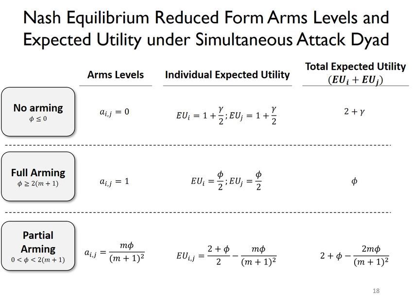
the stage from the previous section in which both players simultaneously choose how
much of their resource endowment to consume versus how much to spend on arms.
After this first stage, both players observe each side’s arms levels and then the game
continues into a second stage that is identical to the one stage game described in the
previous section.
 In addition, these two stages are now infinitely repeated. As before, if the game
results in any of the war equilibria, there is a decisive war in which one side wins and
gets the winning payoff in perpetuity while the losing side is eliminated and gets a
payoff of 0 henceforth. If the game results in peace, however, the game continues to
the next time period where these two stages are repeated again. Following Fearon, we
will assume that when peace is an equilibrium, players will engage in an unspecified
bargaining process over international issues < 1 where bargaining power is a
function of arms levels and is allocated according to the bargaining CSF ( , ),
which meets the conditions specified in Fearon 2018. When war is an equilibrium,
the winning state will gain full control of .
 A summary of this dynamic model with endogenous arms levels and exogenous
war costs is shown in Figure 3.

 17

18
 FIGURE 3. Dynamic Model with Endogenous Arming and Exogenous War Costs in Extensive Form

In his 2018 model, Fearon argued that the arms spending required to maintain
peace through deterrence represents a theoretically defensible measure for the costs
of anarchy in peace: military spending is wasteful since it cannot be consumed to
increase welfare. In our model, we generalize Fearon’s costs of anarchy concept to
cover outcomes in both peace and war equilibria. We define welfare as the present
value (PV) of states’ payoffs in some outcome. We define the costs of anarchy as
the difference between the PV of a state’s payoffs in that outcome and the PV of a
state’s payoffs in the maximum cooperation outcome in which states exist in a state of
perpetual peace with no arms spending and evenly split international issues. The lower
a state’s welfare, the higher the costs of anarchy.49 This extended model is now able
to consider the costs of anarchy under both war and peace scenarios. We retain the
assumption from the previous section that the two states have identical preferences and
their payoffs are measured in units of their identical resource endowments. Therefore,
we can make interstate comparisons of welfare. We will throughout this analysis
consider total welfare, which is the aggregate of the PV of both states’ payoffs.
 As in the one-shot game, a peace equilibrium can be supported if each sides’ arms
levels are high enough such that they deter the other side from engaging in a predatory
attack. The difference here is that arms are now an endogenous choice. In order for a
peaceful equilibrium to be feasible, there must exist some ˆ ∈ [0, 1] that meets the
following dynamic war constraint condition:

 1 − ˆ + /2 − + (1 + )
 ≥ max 1 − + ( , ;
 ˆ ) (3)
 (1 − ) (1 − )
 The LHS of the dynamic war constraint represents a state’s welfare when it chooses
arms level ˆ and neither side attacks in every period. The RHS of the war constraint
represents the welfare of a state that makes a predatory attack on another state that
chooses arms level , ˆ and where the attacking state’s arms levels are chosen to
maximize their welfare. As long as there exists some ˆ that satisfies this dynamic war
constraint, then a subgame perfect Nash equilibrium (SPNE) with perpetual peace can
be supported. This is because if a state i chooses arms level = ,
 ˆ then an opponent
j may consider arming up to attack, but that opponent could achieve higher expected
utility by also spending = ˆ and not attacking. Following Fearon, we focus on the
Pareto Optimal (undominated) SPNE of the game. When the dynamic war constraint
can be satisfied, the Pareto Optimal SPNE is a peaceful equilibrium in which states
choose the a* that solves the war constraint with equality in every period. This a* is
the arms level that allows states to maximize their consumption by minimizing their
arms burden while maintaining deterrence against a predatory attack. As we showed
in the previous section, satisfying the war constraint is a necessary but not sufficient

 49. Because the factors determining state payoffs are given exogenously with the exception of arms
spending, the PV of a state’s payoffs in the maximum cooperation outcome in which there is no arms
spending outcome is given exogenously. Therefore, higher welfare is synonymous with lower costs of
anarchy. We generally measure outcomes in terms of welfare in this paper.

 19

condition for peace. When offense is advantaged ( > 1) and the war constraint is
satisfied (i.e. scenario 3: Security Dilemma), there are always equilibria where both
players attack because they expect the other side to attack. However, simultaneous
attack in scenario 3 is Pareto dominated by peace. When there are multiple SPNE, the
focus of the welfare analysis in this section is on the Pareto Optimal SPNE. When
defense is advantaged ( < 1) and the war constraint is satisfied (i.e. scenario 4:
Stable Deterrence), then perpetual peace is the only SPNE outcome.50
 Following Fearon, we make the assumption that the Nash Equilibrium arms levels
( ) are larger than a* when peace is an equilibrium. Functionally, this allows
us to determine a single Pareto Optimal SPNE value for arms levels and to avoid
equilibria with random arms levels and a positive chance of attack that were described
in (Jackson 2009).51
 If there does not exist some ˆ ∈ [0, 1] that satisfies the dynamic war constraint, this
implies that there is not a peaceful SPNE because an opponent’s best response will be to
arm up and attack the non-attacking state. In this case, any SPNE involves: immediate
war where both players choose arms levels to maximize their expected payoffs in the
war. If > 1, then this corresponds with the Offensive War scenario described in
the previous section. If < 1, then this corresponds with the Rope-A-Dope scenario
from the previous section.
 In addition, we must reconsider the Pyrrhic Victory condition because arming is
now an endogenous choice.52 An attacker can only succeed with 100% certainty if the
opponent chooses to spend none of its resource endowment on arms. In this case, the
attacker could spend some very small > 0 on arms and achieve victory with 100%
certainty. Therefore, the Pyrrhic victory condition in this iteration of the model with
endogenous arming and exogenous war costs becomes:

 1 + /2 − + (1 + )
 > 1+
 1− 1− 
 This simplifies to:
 
 > + (4)
 2

 50. Fearon claimed that there are always equilibria where both sides attack because they expect the
other side to attack even though this outcome is Pareto dominated by a feasible peaceful outcome (Fearon
2018, footnote 23). However, this is only the case when offense is advantaged ( > 1). When defense is
advantaged, states have a higher probability of winning when they are attacked than when they attack, and
therefore (attack,attack) is not part of an SPNE.
 51. See (Fearon 2018) for more detail on the role of the bargaining process. As with Fearon’s original
analysis, peaceful equilibria result in symmetric arming and an even split of . As in Fearon’s model, the
bargaining process only plays a subtle role when states are given the option to attack in that it keeps states
from undercutting on military spending, since this would disadvantage them on bargaining. This thus rules
out equilibria with random arms levels found in (Jackson 2009), which would significantly complicate our
welfare analysis.
 52. The Pyrrhic Victory condition in this iteration of the model is the complement of equation 2 from
(Fearon 2018)

 20