Human Inference in Changing Environments With Temporal Structure
←
→
Page content transcription
If your browser does not render page correctly, please read the page content below
Human Inference in Changing Environments With Temporal
                                                                         Structure
                                             Arthur Prat-Carrabin1,† , Robert C. Wilson3,‡ , Jonathan D. Cohen3 , and Rava Azeredo da
                                                                                  Silveira1,2,3,4*
arXiv:2101.11143v1 [q-bio.NC] 27 Jan 2021

                                              1
                                                Laboratoire de Physique de l’École Normale Supérieure, ENS, Université PSL, CNRS,
                                                              Sorbonne Université, Université de Paris, 75005 Paris, France
                                                           2
                                                             IOB, Faculty of Science, University of Basel, Basel, Switzerland
                                                      3
                                                        Princeton Neuroscience Institute, Princeton University, Princeton, USA
                                                   4
                                                     Department of Neurobiology, Weizmann Institute of Science, Rehovot, Israel
                                                      †
                                                        Present address: Department of Economics, Columbia University, USA
                                            ‡
                                              Present address: Department of Psychology and Cognitive Science Program, University of
                                                                                 Arizona, Tucson, USA
                                                                           *
                                                                             For correspondence: rava@ens.fr

                                                                                               Abstract
                                                       To make informed decisions in natural environments that change over time, humans must
                                                   update their beliefs as new observations are gathered. Studies exploring human inference as a
                                                   dynamical process that unfolds in time have focused on situations in which the statistics of ob-
                                                   servations are history-independent. Yet temporal structure is everywhere in nature, and yields
                                                   history-dependent observations. Do humans modify their inference processes depending on the
                                                   latent temporal statistics of their observations? We investigate this question experimentally and
                                                   theoretically using a change-point inference task. We show that humans adapt their inference
                                                   process to fine aspects of the temporal structure in the statistics of stimuli. As such, humans
                                                   behave qualitatively in a Bayesian fashion, but, quantitatively, deviate away from optimality.
                                                   Perhaps more importantly, humans behave suboptimally in that their responses are not deter-
                                                   ministic, but variable. We show that this variability itself is modulated by the temporal statistics
                                                   of stimuli. To elucidate the cognitive algorithm that yields this behavior, we investigate a broad
                                                   array of existing and new models that characterize different sources of suboptimal deviations
                                                   away from Bayesian inference. While models with ‘output noise’ that corrupts the response-
                                                   selection process are natural candidates, human behavior is best described by sampling-based
                                                   inference models, in which the main ingredient is a compressed approximation of the posterior,
                                                   represented through a modest set of random samples and updated over time. This result comes
                                                   to complement a growing literature on sample-based representation and learning in humans.

                                            ©2021, American Psychological Association. This paper is not the copy of record and may not exactly
                                            replicate the final, authoritative version of the article. Please do not copy or cite without authors’ permission.
                                            The final article will be available, upon publication, via its DOI: 10.1037/rev0000276

                                                                                                    1
In a variety of inference tasks, human subjects use sensory cues as well as prior information in
a manner consistent with Bayesian models. In tasks requiring the combination of a visual cue
(such as the shape, position, texture, or motion of an object) with a haptic [1, 2], auditory [3],
proprioceptive [4], or a secondary visual cue [5, 6, 7], human subjects weigh information coming
from each cue according to its uncertainty, in agreement with an optimal, probabilistic approach.
Moreover, subjects appear also to integrate optimally prior knowledge on spatial [8, 9] and temporal
[10, 11] variables relevant to inference, in line with Bayes’ rule.
The Bayesian paradigm hence offers an elegant and mathematically principled account of the
way in which humans carry inference in the presence of uncertainty. In most experimental designs,
however, successive trials are unrelated to each other. Yet, in many natural situations, the brain
receives a stream of evidence from the environment: inference, then, unfolds in time. Moreover,
natural mechanisms introduce sophisticated temporal statistics in the course of events (e.g., rhyth-
micity in locomotion, day-night cycles, and various structures found in speech). Are these temporal
dynamics used by the brain to refine its online inference of the state of the environment?
Furthermore, most studies that support a Bayesian account of human inference discuss average
behaviors of subjects, and, thereby, side-step the issue of the variability in human responses. While
an optimal Bayesian model yields a unique, deterministic action in response to a given set of obser-
vations, human subjects exhibit noisy, and thus suboptimal, responses. Methods commonly used to
model response variability, such as ‘softmax’ and probability-matching response-selection strategies,
or, more recently, stochastic inference processes, correspond to different forms of departure from
Bayesian optimality. One would like to identify the nature of the deviations from Bayesian models
that can account for the observed discrepancies from optimality in human behavior.
To explore these questions, we use an online inference task based on a ‘change-point’ paradigm,
i.e., with random stimuli originating from a hidden state that is subject to abrupt, occasional vari-
ations, which are referred to as ‘change points’. A growing theoretical and experimental literature
examines inference problems for this class of signals [12, 13, 14, 15, 16, 17, 18, 19, 20, 21, 22, 23, 24,
25, 26]. All these studies, with the exception of the work of [13], focus on the history-independent
case of random change points that obey Poisson temporal statistics. Such problems are character-
ized by the absence of temporal structure: the probability of occurrence of a change point does not
depend on the realization of past change points. [15, 23] and [22] extend their studies beyond this
simple framework by considering ‘hierarchical-Poisson’ models in which the change probability is
itself subject to random variations; but, here also, the occurence of a change point does not depend
on the timing of earlier change points. The experimental studies among the ones cited above have
investigated the way in which human subjects and rodents infer hidden states, and whether they
learn history-independent change probabilities.
Because of the pervasiveness of temporal structure in natural environments, we decided to study
human inference in the presence of ‘history-dependent’ statistics in which the occurrence of a change
point depends on the timing of earlier change points. This introduces considerable complexity in
the optimal inference model (as the hidden state is no longer Markovian), and serves as a first step
toward a more ecological approach to human inference. For the purpose of comparison, we consider
two different statistics of change points: the first one is the Poisson statistics commonly used in
earlier studies; the second is the simplest non-Markovian statistics, in which the probability of a
change point is a function of the timing of the preceding change point. This setup allows us to
examine the effect of the latent temporal structure on both human behavior and model responses.
In these two contrasting conditions, the behavior of the Bayesian model and that of human
subjects exhibit both similarities and discrepancies. A salient departure from optimality exhibited
2by subjects is the variability in their responses. What is more, the shape of the distribution of
responses is not constant, but, rather, subject to modulations during the course of inference. The
standard deviation and skewness of the empirical response distribution are correlated with that
of the optimal, Bayesian posterior; this suggests that the randomness in subjects’ responses does
not reflect some ‘passive’ source of noise but is in fact related to the uncertainty of the Bayesian
observer.
To account for this non-trivial variability in human responses and other deviations from opti-
mality, we investigate in what ways approximations of the Bayesian model alter behavior, in our
task. The optimal estimation of a hidden state can be split into two steps: Bayesian posterior
inference (computing optimally the belief distribution over the state space) and optimal response
selection (using the belief distribution to choose the response that maximizes the expected reward).
Suboptimal models introduce systematic errors or stochastic errors in the inference step or in the
response-selection step, or in both, thus impacting behavior. Models discussed in the change-point
literature, along with new models we introduce, provide a wide range of such deviations from op-
timality, which we compare to experimental data. This allows us to assess how different sources of
suboptimality impact behavior, and to what extent they can capture the salient features in human
behavior.
The paper is outlined as follows. We first present the main aspects of our task, in which subjects
observe a visual stimulus and infer an underlying, changing, hidden state. The susceptibility of
subjects to a new stimulus is shown to differ appreciably between the two conditions (with and
without latent temporal structure), and to adapt to the statistics of change points. We then analyze
the variability in the subjects’ responses, and show how it is modulated over the course of inference.
After deriving the optimal, Bayesian solution of the inference problem in the context of our task,
we examine its behavior in comparison with experimental data. We then turn to investigating a
broad family of suboptimal models. In particular, motivated by the form of the variability present
in our human data, we examine stochastic perturbations in both the inference step and in the
response-selection step. These models reflect different forms of sampling: model subjects either
perform inference using samples of probability distributions or select responses by sampling; the
former option includes models with limited memory as well as sequential Monte Carlo (particle-
filter) models. Finally, we discuss model fitting, from which we conclude that humans carry out
stochastic approximations of the optimal Bayesian calculations through sampling-based inference
(rather than sampling-based response selection).
Our observations confirm and extend the results reported in the change-point literature on
human inference in the context of Poisson statistics, by exploring a more ecological [27, 28, 29, 30,
31, 32, 33, 34, 35], non-Poisson, temporally structured environment. Likewise, our results come to
complement those of a number of studies on perception and decision-making that also investigate
inference from stimuli with temporal statistics [36, 37, 38, 10, 11, 39]. Our experimental results
demonstrate that humans learn implicitly the temporal statistics of stimuli. Moreover, our work
highlights the variability ubiquitous in behavioral data, and shows that it itself exhibits structure:
it depends on the temporal statistics of the signal, and it is modulated over the course of inference.
We find that a model in which the Bayesian posterior is approximated with a set of samples captures
the behavioral variability during inference. This proposal adds to the growing literature on cognitive
‘sample-based representations’ of probability distributions [40, 41, 42, 43]. Our results suggest that
the brain carries out complex inference by manipulating a modest number of samples, selected as a
low-dimensional approximation of the optimal, Bayesian posterior.
31 Results
1.1 Behavioral task, and history-independent vs. history-dependent stimuli
In our computer-based task, subjects are asked to infer, at successive trials, t, the location, on
a computer screen, of a hidden point, the state, st , based on an on-screen visual stimulus, xt ,
presented as a white dot on a horizontal line (Fig. 1A,B). Subjects can only observe the white
dots, whose positions are generated around the hidden state according to a likelihood probability,
g(xt |st ) (Fig. 1C,E, blue distribution). The state itself, st , follows a change-point process, i.e., it is
constant except when it ‘jumps’ to a new location, which happens with probability qt (the ‘hazard
rate’ or ‘change probability’). The dynamics of change points are, hence, determined by the change
probability, qt . To examine the behavior of models and human subjects in different ‘environments’,
we choose two kinds of signals which differ in their temporal structure. History-independent (HI)
signals are memoryless, Poisson signals: qt is constant and equal to 0.1. Consequently, the intervals
between two change points last, on average, for 10 trials, and the distribution of these intervals is
geometric (Fig. 1D, blue bars). Conversely, history-dependent (HD) signals are characterized by
temporal correlation. Change points also occur every 10 trials, on average, but the distribution
of the duration of inter-change-point intervals is peaked around 10. This corresponds to a change
probability, qt , that is an increasing function of the number of trials since the last change point —
a quantity referred to as the ‘run-length’, τt . We thus denote it by q(τt ). In HD signals, change
points occur in a manner similar to a ‘jittered periodic’ process, though the regularity is not readily
detected by subjects.
When a change point occurs, the state randomly jumps to a new state, st+1 , according to a state
transition probability, a(st+1 |st ) (Fig. 1C,E, green distribution). The likelihood, g, and the state
transition probability, a, overlap, thus allowing for ambiguity when a new stimulus is viewed: is it
a random excursion about the current state, or has the state changed? At each trial, subjects click
with a mouse to give their estimate, ŝt , of the state. The reward they receive for each response is
a decreasing function, R, of the distance between the state and the estimate, |ŝt − st |: one reward
point if the estimate falls within a given, short distance from the state, 0.25 point if it falls within
twice that distance, and 0 point otherwise (Fig. 1E). The task is presented as a game to subjects:
they are told that someone is throwing snowballs at them. They cannot see this hidden person
(whose location is the state, st ), but they observe the snowballs as white dots on the screen (the
stimulus, xt ). After several tutorial runs (in some of which the state is shown), they are instructed
to use the snowballs to guess the location of the person (i.e., produce an estimate, ŝt ). Additional
details on the task are provided in Methods.
1.2 Learning rates adapt to the temporal statistics of the stimulus
A typical example of a subject’s responses is displayed in Fig. 2A. To describe the data, we focus,
throughout this paper, on three quantities: the learning rate, defined as the ratio of the ‘correction’,
ŝt+1 − ŝt , to the ‘surprise’, xt+1 − ŝt ; the repetition propensity, defined as the proportion of trials
in which the learning rates vanishes (ŝt+1 = ŝt ); and the standard deviation of the responses of the
subjects. The learning rate represents a normalized measure of the susceptibility of a subject to a
new stimulus. If the new estimate, ŝt+1 , is viewed as a weighted average of the previous estimate,
ŝt , and the new stimulus, xt+1 , the learning rate is the weight given to xt+1 . A learning rate of 0
means that the subject has not changed its estimate upon observing the new stimulus; a learning
rate of 0.5 means that the new estimate is equidistant from the previous estimate and the new
stimulus; and a learning rate of 1 means that the new estimate coincides with the new stimulus,
and the past is ignored (Fig. 2A).
4Change-point stimulus
C 10
Signal xt
8
6 State st
4
2
0
10
8 Change probability qt(τt)
6
Run-length τ
4
2
T ime
0
8
State transition probability at(st+1|st)
6
4
2
0
10
8
6
4
Likelihood g(xt|st)
2
0
0 0.25 0.5 0.75 1 -20 -10 0 10 20
1.0
D E g(xt|st)
HI a(st+1|st)
q(τ)
0.5
HD
0.1
0.3
p(interval)
0.2 0.25pt
0.1 1pt
0 5 10 15 20 60 70 80 90 100 110 120 130 140
Run-length τ st, xt, st+1
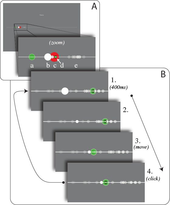
Figure 1: Inference task and change probability, q, in the HI and HD conditions. A. The various
elements in the task appear on a horizontal white line in the middle of a gray screen. a: subject’s pointer
(green disk). b: new stimulus (white disk). c: state (red disk, only shown during tutorial runs). d: position
of subject’s previous click (green dot). e: for half of subjects, previous stimuli appear as dots decaying with
time. B. Successive steps of the task: 1, 2: a new stimulus is displayed; to attract the subject’s attention,
it appears as a large, white dot for 400ms, after which it becomes smaller. 3: the subject moves the pointer.
4: The subject clicks to provide an estimate of the position of the state. After 100ms, a new stimulus
appears, initiating the next trial. C. The position of the stimulus on the horizontal axis, xt , is generated
randomly around the current state, st , according to the triangle-shaped likelihood function, g(xt |st ). The
state itself is constant except at change points, at which a new state, st+1 , is generated around st from the
bimodal-triangle-shaped transition probability, a(st+1 |st ). The run-length, τt , is defined as the number of
trials since the last change point. Change points occur with the change probability q(τt ) (orange bars), which
depends on the run-length in the HD condition (depicted here). D. Top panel: change probability, q(τ ), as a
function of the run-length, τ . It is constant and equal to 0.1 in the HI condition, while it increases with the
run-length in the HD condition. Consequently, the distribution of intervals between two consecutive change
points (bottom panel) is geometric in the HI condition whereas it is peaked in the HD condition; in both
conditions, the average duration of inter-change-point intervals is 10. E. Compared extents of the likelihood,
g(xt |st ) (green), the state transition probability, a(st+1 |st ) (blue), the ‘shot’ resulting from a click (green
dot), and the radii of the 1-point (red disk) and 0.25-point (grey circle) reward areas. A shot overlapping
the red (gray) area yields 1 (0.25) point.
5A Learning Rate ≈ 0.5
160 State Subject 13
Signal
140 Learning Rate ≈ 0
Learning Rate ≈ 1
120
100 Surprise Correction
Correction
Learning Rate =
Surprise
80
t
B ∗∗∗ C
∗∗ HI HD
Average learning rate
0.30 ∗∗ 0.35
∗∗ ∗
Learning rate
∗
0.30 ∗
0.20 ∗ ∗
∗ ∗
0.25
0.10
0.20
0.00
HI HI HD HD 0 2 4 6 8 10
τ̃ ∈ [5, 6] τ̃ ∈ [9, 10] τ̃ ∈ [5, 6] τ̃ ∈ [9, 10] Run-length τ̃
Figure 2: Human learning rates depends on the temporal statistics (HI or HD) of the stimulus.
A. Illustration of the learning rate using a sample of a subject’s responses (red line). The ‘surprise’ (blue
arrow) is the difference, xt+1 − ŝt , between the estimate at trial t, ŝt (red), and the new stimulus at trial t+1,
xt+1 (blue). The ‘correction’ (red arrow) is the difference between the estimate at trial t and the estimate
at trial t + 1, ŝt+1 − ŝt . The ‘learning rate’ is the ratio of correction to surprise. B. Average learning rates in
HI (blue) and HD (orange) conditions, at short run-lengths (τ̃ ∈ [5, 6]) and long run-lengths (τ̃ ∈ [9, 10]). In
the HD condition the change probability increases with the run-length, which advocates for higher learning
rates at long run-lengths. C. Average learning rates in HI (blue) and HD (orange) conditions, vs. run-length
τ̃ . Shaded bands indicate the standard error of the mean. B,C. Stars indicate p-values of one-sided Welch’s
t-tests, which do not assume equal population variance. Three stars: p < 0.01; two stars: p < 0.05; one
star: p < 0.1. Bonferroni-Holm correction [44] is applied in panel B.
Our data show that for human subjects the learning rate is not constant, and can vary from no
correction at all (learning rate ≈ 0) to full correction (learning rate ≈ 1). We investigated how the
average learning rate behaved in relation to the run-length, in the HI and HD conditions. As the
run-length is not directly accessible to subjects, in our analyses we used the empirical run-length,
τ̃ , a similar quantity derived from the subjects’ data (see Methods). Unless otherwise stated, we
focus our analyses on cases in which the surprise, xt+1 − ŝt , is in the [8,18] window, in which there
is appreciable ambiguity in the signal.
A first observation emerging from our data is that the learning rate changes with the run-
length, in a quantitatively different fashion depending on the condition (HI or HD). In the HI
condition, learning rates at short run-length (τ̃ ∈ [5, 6]) are significantly higher than at long run-
length (τ̃ ∈ [9, 10]), i.e., the learning rate decreases with run-length (Fig. 2B, blue bars). In
the HD condition, the opposite occurs: learning rates are significantly higher at long run-lengths
(Fig. 2B, orange bars), indicating that subjects modify their inference depending on the temporal
6structure of the signal. In addition, at short run-lengths, learning rates are significantly lower in
the HD condition than in the HI condition; this suggests that subjects take into account the fact
that a change is less likely at short run-lengths in the HD condition. The opposite holds at long
run-lengths: HD learning rates are markedly larger than HI ones (Fig. 2B).
Inspecting the dependence of the learning rate on the run-length (Fig. 2C), we note that the
HD learning-rate curve adopts a ‘smile shape’, unlike the monotonic curve in the HI condition.
(A statistical analysis confirms that these curves have significantly different shapes; see Methods.)
The HI curve is consistent with a learning rate that simply decreases as additional information
is accumulated on the state. In the HD condition, initially the learning rate is suppressed, then
boosted at longer run-lengths, reflecting the modulation in the change probability.
These observations demonstrate that subjects adapt their learning rate to the run-length, and
that in the HD condition subjects make use of the temporal structure in the signal. These results
are readily intuited: shortly after a change point, the learning rate should be high, as little is
known about the new state, while at longer run-lengths the learning rate should tend to zero as the
state is more and more precisely inferred. This decreasing behavior is observed, but only in the HI
condition. The HD condition introduces an opposing effect: as the run-length grows, new stimuli are
increasingly likely to divulge the occurrence of a new state, which advocates for adopting a higher
learning rate. This tradeoff is reflected in our data in the ‘smile shape’ of the HD learning-rate curve
(Fig. 2C; these trends subsist at longer run-lengths, see Supplementary Fig. 17.). The increase in
learning rate at long run-lengths is reminiscent of the behavior of a driver waiting at a red light:
as time passes, the light is increasingly likely to turn green; as a result, the driver is increasingly
susceptible to react and start the car.
1.3 Human repetition propensity
A closer look at the data presented in the previous section reveals that in a number of trials the
learning rate vanishes, i.e., ŝt+1 = ŝt . The distribution of the subjects’ corrections, ŝt+1 − ŝt ,
exhibits a distinct peak at zero (Fig. 3A). In other words, in a fraction of trials, subjects click
twice consecutively on the same pixel. We call such a response a ‘repetition’, and the fraction of
repetition trials the ‘repetition propensity’. The latter varies with the run-length: it increases with
τ in both HI and HD conditions, before decreasing in the HD condition for long run-lengths (Fig.
3B).
What may cause the subjects’ repetition behavior? The simplest explanation is that, after
observing a new stimulus, a subject may consider that the updated best estimate of the state lands
on the same pixel as in the previous trial. The width of one pixel in arbitrary units of our state
space is 0.28. As a comparison, the triangular likelihood, g, has a standard deviation, σg , of 8.165.
An optimal observer estimating the center of a Gaussian density of standard deviation σ√ g , using 10
samples from this density, comes up with a posterior density with standard deviation σg / 10 ≈ 2.6.
Therefore, after observing even 10 successive stimuli, the subjects’ resolution is not as fine as a pixel
(it is, in fact, 10 times coarser). This indicates that the subjects’ repetition propensity is higher
than the optimal one (the behavior of the optimal model, presented below, indeed exhibits a lower
average repetition propensity than that of the subjects). Another possible explanation is that even
though the new estimate falls on a nearby location, a motor cost prohibits a move if it is not
sufficiently extended to be ‘worth it’ [45, 46, 47, 48]. A third, heuristic explanation is that humans
are subject to a ‘repetition bias’ according to which they repeat their response irrespective of their
estimate of the state.
Regardless of its origin, the high repetition propensity in data raises the question of whether
it dominates the behavior of the average learning rate. As a control, we excluded all occurrences
7A HI
HD
Histogram −15 −10 −5 0 5 10 15
Corrections
B
25%
Repetition propensity
*
* *
*
20%
HI
15%
HD
10%
0 2 4 6 8 10
Run-length
Figure 3: Human repetition propensity depends on the temporal statistics, and dynamically
on the run-length. A. Histogram of subject corrections (difference between two successive estimates,
ŝt+1 − ŝt ), in the HI (blue) and HD (orange) conditions. The width of bins corresponds to one pixel on the
screen, thus the peak at zero represents the repetition events (ŝt+1 = ŝt ). B. Repetition propensity, i.e.,
proportion of occurrences of repetitions in the responses of subjects, as a function of run-length, in the HI
(blue) and HD (orange) conditions. Stars indicate p-values of Fisher’s exact test of equality of the repetition
propensities between the two conditions, at each run-length.
of repetitions in subjects’ data and carried out the same analyses on the truncated dataset. We
reached identical conclusions, namely, significant discrepancies between the HI and HD learning rates
at short and long run-lengths, albeit with, naturally, higher average rates overall (see Supplementary
Fig. 18).
1.4 The variability in subjects’ responses evolves over the course of inference
In the previous two sections, we have examined two aspects of the distribution of responses: the
average learning rate and the probability of response repetition. We now turn to the variability in
subjects’ responses. Although all subjects were presented with identical series of stimuli, xt , their
responses at each trial were not the same (Fig. 4A). This variability appears in both HI and HD
conditions. The distribution of responses around their averages at each trial has a width comparable
to that of the likelihood distribution, g(xt |st ) (Fig. 4B). More importantly, the variability in the
responses (as measured by the standard deviation) is not constant, but decreases with successive
trials following a change point, at short run-lengths (Fig. 4C). Comparing the HI and HD conditions,
we observe that for run-lengths shorter than 7, the standard deviation in the HD condition is
significantly lower than that in the HI condition. At longer run-lengths, the two curves cross and
the variability in the HD condition becomes significantly higher than in the HI condition. The
8HD curve adopts, again, a ‘smile shape’ (Fig. 4C). What is the origin of the response variability?
Because it changes with the run-length and the HI vs. HD condition, it cannot be explained merely
be the presence of noise independent from the inference process, such as pure motor noise. In order
to encompass human behavior in a theoretical framework and to investigate potential sources of
this inference-dependent variability, we start by comparing the recorded behavior with that of an
optimal observer.
1.5 Optimal estimation: Bayesian update and maximization of expected reward
We derive the optimal solution for the task of estimating the hidden state, st , given random stimuli,
xt . The first step (the ‘inference step’) is to derive the optimal posterior distribution over the
state, st , using Bayes’ rule. Because the state is a random variable coupled with the run-length,
τt , another random variable, it is convenient to derive the Bayesian update equation for the (st , τt )
pair (more precisely, the (st , τt ) pair verifies the Markov property, whereas st alone does not, in the
HD condition). We denote by x1:t the string of stimuli received between trial 1 and trial t, and by
pt (s, τ |x1:t ) the probability distribution over (s, τ ), at trial t, after having observed the stimuli x1:t .
At trial t + 1, Bayes’ rule yields pt+1 (s, τ |x1:t+1 ) ∝ g(xt+1 |s)pt+1 (s, τ |x1:t ). Furthermore, we have
the general transition equation,
XZ
pt+1 (s, τ |x1:t ) = pt+1 (s, τ |st , τt )pt (st , τt |x1:t )dst , (1)
τt st
given by the change-point statistics. As the transition probability, pt+1 (s, τ |st , τt ), can be expressed
using q(τt ) and a(s|st ) (see Methods for details), we can reformulate the update equation as
"
1
Z
g(xt+1 |s) 1τ =0
X
pt+1 (s, τ |x1:t+1 ) = q(τt ) a(s|st )pt (st , τt |x1:t )dst
Zt+1 τt s t
# (2)
+1τ >0 (1 − q(τ − 1))pt (s, τ − 1|x1:t ) ,
where 1C = 1 if condition C is true, 0 otherwise; and Zt+1 is a normalization constant. This equation
includes two components: a ‘change-point’ one (τ = 0) and a ‘no change-point’ one (τ > 0). We
call the model that performs this Bayesian update of the posterior the OptimalInference model.
Finally, following the inference step just presented (i.e., the computation of the posterior), a
‘response-selection step’ determines
R the behavioral response. At trial t and for a response ŝt , the
expected reward is Es R = R(|ŝt − s|)pt (s|x1:t )ds. The optimal strategy selects the response, ŝt ,
that maximizes this quantity. Before exploring the impact of relaxing the optimality in the inference
step, in the response-selection step, or both, we examine, first, the behavior of the optimal model.
1.6 The optimal model captures qualitative trends in learning rate and repeti-
tion propensity
Equipped with the optimal model for our inference task, we compare its output to experimental
data. For short run-lengths (τ < 8), the learning rates in both HI and HD conditions decrease as a
function of the run-length, and the HD learning rates are lower than their HI counterparts. They
increase, however, at longer run-lengths (τ ≥ 8) and ultimately exceed the HI learning rates; these,
by contrast, decrease monotonically (Fig. 5A, solid line). These trends are similar to those observed
in behavioral data (Fig. 5A, dashed line). Hence, the modulation of the subjects’ learning rates
9A
t State st
Signal xt
Estimates ŝt
ŝt distribution
90 95 100 105 110 115 120 125 130
st, xt, ŝt
B Distribution of responses around average
g(xt|st)
a(st+1|st)
Responses
Histogram
−20 −10 0 10 20
Distance to st or to average response
C 7.0
V ariability of responses
∗
HI HD ∗
∗
Standard deviation
6.5 ∗
∗
∗
6.0 ∗ ∗
∗ ∗
∗ ∗
5.5 ∗ ∗ ∗
∗ ∗ ∗
∗
∗
5.0
4.5
0 2 4 6 8 10
Run-length τ̃
Figure 4: The variability in subjects’ responses is modulated during inference, and these
modulations depend on the temporal statistics of the stimulus. A. Responses of subjects in an
example of 5 consecutive stimuli. In this example, there is no change point and the state (green) is constant.
At each trial (from top to bottom), subjects observe the stimuli (blue) and provide their responses (red
bars). A histogram of the locations of the responses is obtained by counting the number of responses in bins
of width 3 (light red). B. Distribution of the responses of subjects around their average (red), compared
to the likelihood, g (blue), and the state transition probability, a (green). C. Standard deviation of the
responses of subjects vs. run-length, τ̃ , in the HI (blue) and HD (orange) conditions. Stars indicate p-value
of Levene’s test of equality of variance between the two conditions, at each τ̃ . Shaded bands indicate the
standard error of the standard deviation [49].
with the temporal statistics of the stimuli, and over the course of inference, is consistent, at least
qualitatively, with that of a Bayesian observer.
Although a Bayesian observer can, in principle, hold a continuous posterior distribution, we
discretize, instead, the posterior, in order to reproduce the experimental condition of a pixelated
10A Learning rate B30% Repetition propensity C Standard deviation
0.4 HI Subjects 6.0
HD OptimalInf erence
20%
0.3 4.0
0.2
10% 2.0 Bayesian P osterior (pdf )
0.1
0% 0.0
0 2 4 6 8 10 0 2 4 6 8 10 0 2 4 6 8 10
Run-length Run-length Run-length
Figure 5: The optimal model captures qualitatively the behavior of the learning rate and of the
repetition propensity in subjects, but does not account for their variability. A. Average learning
rate as a function of the run-length. In the HI condition, the learning rate decreases with the run-length, for
both the optimal model and the subjects. In the HD condition, learning rates in the optimal model are lower
than in the HI condition, for short run-lengths, and higher for long run-lengths. The learning rate of subjects
exhibits a similar smile shape, in the HD condition. B. Repetition propensity, i.e., proportion of repetition
trials, as a function of the run-length. C. Standard deviation of the responses of the subjects (dashed lines)
and of the optimal model (solid lines), and standard deviation of the optimal, Bayesian posterior distribution
(long dashes), as a function of the run-length. The optimal model is deterministic and, thus, exhibits no
variability in its responses. The optimal posterior distribution, however, has a positive standard deviation
which decreases with the run-length, in the HI condition, and exhibits a smile shape, in the HD condition.
screen. This discretization allows for repetitions. The repetition propensity of the optimal model
varies with the run-length: it increases with τ in both HI and HD conditions, and decreases in the
HD condition for long run-lengths, a pattern also found in experimental data (Fig. 5B).
Hence, the optimal model captures the qualitative trends in learning rate and repetition propen-
sity present in the responses of the subjects. Quantitative differences, however, remain. The learning
rates of the subjects, averaged over both HI and HD conditions, are 43% higher than the average
learning rate in the optimal model, and the average repetition propensity of the subjects is 9 per-
centage points higher than that in the optimal model.
1.7 Relation between human response variability and the Bayesian posterior
The optimal model captures qualitatively the modulations of learning rate and repetition propensity
in subjects, but it is deterministic (at each trial, the optimal estimate is a deterministic function of
past stimuli) and, as such, it does not capture the variability inherent to the behavior of subjects.
The modulations of the behavioral variability as a function of the run-length and of the temporal
structure of the signal (Fig. 4C) is a sign that the variability evolves as the inference process unfolds.
The standard deviation of the optimal Bayesian posterior decreases with the run-length, in the HI
condition: following a change point, the posterior becomes narrower as new stimuli are observed.
In the HD condition, the standard deviation of the posterior exhibits a ‘smile shape’ as a function
of the run-length: it decreases until the run-length reaches 5, then increases for larger run-lengths
(Fig. 5C). This behavior is similar to that of the standard deviation of the responses of the subjects.
In fact, the standard deviation of the Bayesian posterior and that of subjects’ responses across trials
are significantly correlated, both in the HI condition (Pearson’s r = .53, p < .0001) and in the HD
condition (r = .25, p < .0001). In other words, when the Bayesian posterior is wide there is more
variability in the responses of subjects, and vice-versa (Fig. 6A).
Turning to higher moments of the distribution of subjects’ responses, we find that the skewness
11A 10 Standard deviation B Skewness
HI HI
0.6
9 HD HD
Lin. reg. 0.4 Lin. reg.
8
Subjects Responses
Subjects Responses
0.2
7
0
6
−0.2
5
−0.4
4
−0.6
85% 15% of trials
3
2 4 6 8 10 −3 −2 −1 0 1 2 3
Bayesian posterior Bayesian posterior
Figure 6: Both width and skewness of the distribution of subjects’ responses are correlated
with those of the Bayesian posterior. Empirical standard deviation (A) and skewness (B) of subjects’
responses as a function of the standard deviation and skewness of the Bayesian posterior, in the HI (blue)
and HD (orange) conditions, and linear regressions (ordinary least squares; dashed lines). On 85% of trials,
the standard deviation of the Bayesian posterior is lower than 6.8 (vertical grey line). Shaded bands indicate
the standard error of the mean.
of this distribution appears, also, to grow in proportion to the skewness of the Bayesian posterior
(Fig. 6B). The correlation between these two quantities is positive and significant in the two
conditions (HI: r = .21, p < .0001; HD: r = .14, p < .0001. These results are not driven by
the boundedness of the response domain, which could have artificially skewed the distribution of
response; see Supplementary Fig. 19.). Thus, not only the width, but also the asymmetry in
the distribution of subjects’ responses is correlated with that of the Bayesian posterior. These
observations support the hypothesis that the behavioral variability in the data is at least in part
related to the underlying inference and decision processes.
In what follows, we introduce an array of suboptimal models, with the aim of resolving the
qualitative and quantitative discrepancies between the behavior of the optimal model and that of
the subjects. In particular, we formulate several stochastic models which include possible sources
of behavioral variability. Two scenarios are consistent with the modulations of the magnitude and
asymmetry of the variability with the width and skewness of the Bayesian posterior: stochasticity
in the inference step (i.e., in the computation of the posterior) and stochasticity in the response-
selection step (i.e., in the computation of an estimate from the posterior). The models we examine
below cover both these scenarios.
1.8 Suboptimal models reflecting cognitive limitations
In the previous sections, we have examined the learning rate of the subjects, their repetition propen-
sity, and the variability in their responses; comparison of the behaviors of these quantities to that of
the Bayesian, optimal model, revealed similarities (namely, the qualitative behaviors of the learning
rate and of the repetition propensity) and discrepancies (namely, quantitative differences in these
two quantities, and lack of variability in the optimal model). Although the latter call for a non-
Bayesian account of human behavior, the former suggest not to abandon the Bayesian approach
altogether (in favor, for instance, of ad hoc heuristics). Thus, we choose to examine a family of
sub-optimal models obtained from a sequence of deviations away from the Bayesian model, each of
12which captures potential cognitive limitations hampering the optimal performance.
In the Bayesian model, three ingredients enter the generation of a response upon receiving a
stimulus: first, the belief on the structure of the task and on its parameters; second, the inference
algorithm which produces a posterior on the basis of stimuli; third, the selection strategy which maps
the posterior into a given response. The results presented above, exhibiting the similarity between
the standard deviation of the Bayesian posterior and the standard deviation of the responses of the
subjects (Fig. 5C), points to a potential departure from the optimal selection strategy, in which
the posterior is sampled rather than maximized. This sampling model, which we implement (see
below), captures qualitatively the modulated variability of responses; sizable discrepancies in the
three quantities we examine, however, remain (see Methods). Hence, we turn to the other ingredients
of the estimation process, and we undertake a systematic analysis of the effects on behavior of an
array of deviations away from optimality.
Below, we provide a conceptual presentation of the resulting models; we fit them to experimental
data, and comment on what the best-fitting models suggest about human inference and estimation
processes. For the detailed mathematical descriptions of the models, and an analysis of the ways
in which their predictions depart from the optimal behavior, we refer the reader to the Methods
section.
Models with erroneous beliefs on the statistics of the signal Our first model challenges
the assumption, made in the optimal model, of a perfectly faithful representation of the set of
parameters governing the statistics of the signal. Although subjects were exposed in training phases
to blocs of stimuli in which the state, st , was made visible, they may have learned the parameters
of the generative model incorrectly. We explore this possibility, and, here, we focus on the change
probability, q(τ ), which governs the dynamics of the state. (We found that altering the value of
this parameter had a stronger impact on behavior than altering the values of any of the other
parameters.) In the HD condition, q(τ ) is a sigmoid function shaped by two parameters: its slope,
λ = 1, which characterizes ‘how suddenly’ change points become likely, as a function of τ ; and the
average duration of inter-change-points intervals, T = 10. In the HI condition, q = 0.1 is constant;
it can also be interpreted as an extreme case of a sigmoid in which λ = 0 and T = 1/q = 10. We
implement a suboptimal model, referred to as IncorrectQ, in which these two quantities, λ and T ,
are treated as free parameters, thus allowing for a broad array of different beliefs in the temporal
structure of the signal (Fig. 7A).
Models with limited memory Aside from operating with an inexact representation of the
generative model, human subjects may use a suboptimal form of inference. In the HD condition, the
optimal model maintains ‘in memory’ a probability distribution over the entire (s, τ )-space (see Eq.
(2)), thus keeping track of a rapidly increasing number of possible histories, each characterized by a
sequence of run-lengths. Such a process entails a large computational and memory load. We explore
suboptimal models that alleviate this load by truncating the number of possible scenarios stored in
memory; this is achieved through various schemes of approximations of the posterior distribution.
More specifically, in the following three suboptimal models, the true (marginal) probability of the
run-lengths, pt (τ |x1:t ), is replaced by an approximate probability distribution.
A first, simple way of approximating the marginal distribution of the run-lengths is to consider
only its mean, i.e., to replace it by a Kronecker delta which takes the value 1 at an estimate of
the expected value of the run-lengths. [16] introduce a suboptimal model based on this idea, some
details of which depend on the specifics of the task; we implement a generalization of this model,
adapted to the parameters of our task. We call it the τ Mean model. While the optimal marginal
13A 1
Belief : λ = 0 ; q = cst = 1/T Belief : λ = 0.5 Belief : λ = 1.
T =6 T = 10 T = 20
q(τ )
0.5
0
p(interval)
0.2
0.1
0
1 5 10 15 20 1 5 10 15 20 1 5 10 15 20
B 0.6 1 0.8 0.8
OptimalInf erence τ M ean τ N odes τ M axP rob
t−1
p(τ )
0.3 0.5 0.4 0.4
t
0 0 0 0
0 1 2 3 4 5 6 7 τ̄t−1 τ̄t 2.5 5 0 1 2 3 4 5 6 7
Run-length Expected run-length N odes Run-length
Figure 7: Illustration of the erroneous beliefs in the IncorrectQ model and of the approxi-
mations made in the τ Mean, τ Nodes, and τ MaxProb models. A. Change probability, q(τ ), as a
function of the run-length (first row), and distribution of intervals between two consecutive change points
(second row), for various beliefs on the parameters of the change probability: the slope, λ, and the average
duration of intervals, T . For a vanishing slope (λ = 0), the change probability is constant and equal to 1/T
(first panel). With T = 10 this corresponds to the HI condition (blue lines). For a positive slope (λ > 0),
the change probability increases with the run-length (i.e., a change-point becomes more probable as the time
since the last change-point increases), and the distribution of intervals between two successive change-points
is peaked. The HD condition (orange lines) corresponds to λ = 1 and T = 10. B. Schematic illustration of
the marginal distribution of the run-length, p(τ ), in each model considered. The OptimalInference model
assigns a probability to each possible value of the run-length, τ , and optimally updates this distribution upon
receiving stimuli (first panel). The τ Mean model uses a single run-length which tracks the inferred expected
value, τ̄t (second panel). The τ Nodes model holds in memory a limited number, Nτ , of fixed hypotheses on
τ (“nodes”), and updates a probability distribution over these nodes; Nτ = 2 in this example (third panel).
The τ MaxProb model reduces the marginal distribution by discarding less likely run-lengths; in this example,
2 run-lengths are stored in memory at any given time (fourth panel).
distribution of the run-lengths, pt (τ |x1:t ), spans the whole range of possible values of the run-length,
it is approximated, in the τ Mean model, by a delta function parameterized by a single value, which
we call the ‘approximate expected run-length’ and which we denote by τ̄t . Upon the observation of a
new stimulus, xt+1 , the updated approximate expected run-length, τ̄t+1 , is computed as a weighted
average between two values of the run-length, 0 and τ̄t + 1, which correspond to the two possible
scenarios: with and without a change point at trial t + 1. Each scenario is weighted according to
the probability of a change point at trial t + 1, given the stimulus, xt+1 . This model has no free
parameter (Fig. 7B, second panel).
In a second limited-memory model, contrary to the τ Mean model just presented, the support
of the distribution of the run-lengths is not confined to a single value. This model generalizes the
one introduced by [17]. In this model, the marginal distribution of the run-lengths, pt (τ |x1:t ), is
approximated by another discrete distribution defined over a limited set of constant values, called
‘nodes’ (Fig. 7B, third panel). We call this model τ Nodes. A difference with the previous model
(τ Mean) is that the support of the distribution is fixed, i.e., the set of nodes remains constant
as time unfolds, whereas in the τ Mean model the single point of support, τ̄t , depends on the
14stimuli received. The details of the implementation of this algorithm, and, in particular, of how the
approximate marginal distribution of the run-lengths is updated upon receiving a new stimulus, are
provided in Methods. The model is parameterized by the number of nodes, Nτ , and the values of
the nodes. We implement it with up to five nodes.
The two models just presented are drawn from the literature. We propose a third suboptimal
model that relieves the memory load in the inference process. We also approximate, in this model,
the marginal distribution of the run-lengths, pt (τ |x1:t ), by another, discrete distribution. We call Nτ
the size of the support of our approximate distribution, i.e., the number of values of the run-length
at which the approximate distribution does not vanish. A simple way to approximate pt (τ |x1:t ) is
to identify the Nτ most likely run-lengths, and set the probabilities of the other run-lengths to zero.
More precisely, if, at trial t, the run-length takes a given value, τt , then, upon the observation of
a new stimulus, at trial t + 1 it can only take one of two values: 0 (if there is a change point) or
τt + 1 (if there is no change point). Hence, if the approximate marginal distribution of the run-
lengths at trial t is non-vanishing for Nτ values, then the updated distribution is non-vanishing for
Nτ + 1 values. We approximate this latter distribution by identifying the most unlikely run-length,
arg min pt+1 (τ |x1:t+1 ), setting its probability to zero, and renormalizing the distribution. In other
words, at each step, the Nτ most likely run-lengths are retained while the least likely run-length
is eliminated. We call this algorithm τ MaxProb (Fig. 7B, fourth panel). It is parameterized by
the size of the support of the marginal distribution, Nτ , which can be understood as the number of
‘memory slots’ in the model.
A model with limited run-length memory through sampling-based inference The five
models considered hitherto (OptimalInference, IncorrectQ, τ Mean, τ Nodes, and τ MaxProb) are de-
terministic: a given sequence of stimuli implies a given sequence of responses, in marked contrast
with the variability exhibited in the responses of subjects. To account for this experimental observa-
tion, we suggest several models in which stochasticity is introduced in the generation of a response.
Response stochasticity can stem from the inference step, the response-selection step, or both. We
present, first, a model with stochasticity in the inference step.
This model, which we call τ Sample, is a stochastic version of the τ MaxProb model: instead of
retaining deterministically the Nτ most likely run-lengths at each trial, the τ Sample model samples
Nτ run-lengths using the marginal distribution of the run-lengths, pt (τ |x1:t ). More precisely, if at
trial t + 1 the marginal distribution of the run-lengths, pt+1 (τ |x1:t+1 ), is non-vanishing for Nτ + 1
values, then a run-length is sampled from the distribution [1 − pt+1 (τ |x1:t+1 )] /zt+1 , where zt+1 is a
normalization factor, and the probability of this run-length is set to zero (Fig. 8). In other words,
while the τ MaxProb model eliminates the least likely run-length deterministically, the τ Sample
model eliminates one run-length stochastically, in such a fashion that less probable run-lengths are
more likely to be eliminated. The τ Sample model has one parameter, Nτ , the size of the support
of the marginal distribution of the run-lengths.
Stochastic inference model with sampling in time and in state space: the particle
filter Although the τ Mean, τ Nodes, τ MaxProb, and τ Sample models introduced above relieve the
memory load by prescribing a form of truncation on the set of run-lengths, inference in these models
is still executed on a continuous state space labeled by s (or, more precisely, on a discrete space
with resolution as fine as a pixel). Much as subjects may retain only a compressed representation
of probabilities along the τ axis, it is conceivable that they may not maintain a full probability
function over the 1089-pixel-wide s axis, as they carry out the behavioral task. Instead, they may
infer using a coarser spatial representation, in order to reduce their memory and computational
15p(τ |x1:t ) p(s, τ |x1:t) p(τ |x1:t+1) p(s, τ |x1:t+1) p(τ |x1:t+2) p(s, τ |x1:t+2)
τ =0
τ =1
τ =2
τ =3
τ =4
τ =5
τ =6 OptimalInference
ParticleFilter
τ =7
τ Sample
p(s|x1:t+1)
p(s|x1:t+2)
p(s|x1:t)
xt
xt+1
xt+2
s s s
Figure 8: Posterior density over three successive trials for the OptimalInference model, the
τ Sample model with Nτ = 2, and the ParticleFilter model with ten particles. The three panels
correspond to the three successive trials. Each row except the last one corresponds to a different run-
length, τ . In these rows, the horizontal bars show the marginal probability of the run-length, p(τ |x1:t ). The
posterior (i.e., the joint distribution of the run-length and the state, p(s, τ |x1:t )) is shown as a function of
the state, s, for the OptimalInference model (blue shaded curve), the τ Sample model (pink line), and the
ParticleFilter model (orange vertical bars). The marginal probability of the run-length, p(τ |x1:t ), for the
OptimalInference model, is additionally reflected in the hue of the curve (darker means higher probability).
For the ParticleFilter model, the heights of the bars are proportional to the weights of the particles. When
the state, s, of two or more particles coincide, a single bar is shown with a height proportional to the sum of
the weights. The last row shows the marginal distributions of the states, p(s|x1:t ) = τ p(s, τ |x1:t ), along
P
with the location of the stimulus at each trial (red vertical line). At trial t (left panel), the probability of
the run-length τ = 5 dominates in the three models. In the τ Sample model, it vanishes at run-lengths from
0 to 3, and it is very small for τ = 4. In the ParticleFilter model, the run-lengths of the ten particles are all
5, and thus the probability of all other run-lengths is zero. At trial t + 1 (middle panel), upon observation
of the new stimulus, xt+1 , the marginal probability of the vanishing run-length (τ = 0), which corresponds
to a ‘change-point’ scenario, becomes appreciable in the OptimalInference model (top row). The probability
of the run-length τ = 6 (a ‘no change-point scenario’ ) is however higher. As a result, a ‘bump’ appears in
the marginal distribution of the state, around the new stimulus (bottom row). In the τ Sample model, the
optimal update of the posterior results in a non-vanishing probability for three run-lengths (τ = 0, 5, and 6),
more than the number of ‘memory slots’ available (Nτ = 2). One run-length is thus randomly chosen, and its
marginal probability is set to zero; in the particular instantiation of the model presented here, the run-length
τ = 0 is chosen, and thus the resulting marginal probability of run-length is non-vanishing for τ = 5 and 6
only. In the ParticleFilter model, the stochastic update of the particles results in seven particles adopting
a vanishing run-length, and the probability of a ‘change-point’ scenario (τ = 0) becomes higher than that
of the ‘no change-point’ scenario (τ = 6) supported by the remaining three particles. The various marginal
distributions of the states obtained in these three models (bottom row) illustrate how the τ Sample model
and the ParticleFilter model approximate the optimal posterior: the τ Sample model assigns a negligible
probability to a set of states whose probability is substantial under the OptimalInference model, while the
ParticleFilter yields a coarse approximation reduced to a support of ten states (as opposed to a continuous
distribution).loads. Monte Carlo algorithms perform such approximations by way of randomly sampling the
spatial distribution; sequential Monte Carlo methods, or ‘particle filters’, were developed in the
1990s to address Hidden Markov Models, a class of hidden-state problems within which falls our
inference task [50, 51, 52]. Particle filters approximate a distribution by a weighted sum of delta
functions. In our case, a particle i at trial t is a triplet, (sit , τti , wti ), composed of a state, a run-
length, and a weight; a particle filter with NP particles approximates the posterior, pt (s, τ |x1:t ), by
the distribution
NP
X
p̃t (s, τ |x1:t ) = wti δ(s − sit )δτ,τti , (3)
i=1
where δ(s − sit ) is a Dirac delta function, and δτ,τti a Kronecker delta. In other words, a distribution
over the (s, τ ) space is replaced by a (possibly small) number of points, or samples, in that space,
along with their probability weights.
To obtain the approximate posterior at trial t + 1 upon the observation of a new stimulus, xt+1 ,
we note, first, that the Bayesian update (Eq. (2)) of the approximate posterior, p̃t (s, τ |x1:t ), is a
mixture (a weighted sum) of the NP Bayesian updates of each single particle (i.e., Eq. (2) with the
prior, pt (s, τ |x1:t ), replaced, for each particle, by δ(s − sit )δτ,τti ). Then, we sample independently
each component of the mixture (i.e., each Bayesian update of a particle), to obtain stochastically
the updated particles, (sit+1 , τt+1i ), and to each particle is assigned the weight of the corresponding
component in the mixture. The details of the procedure just sketched, in particular the derivation of
the mixture and of its weights, and how we handle the difficulties arising in practical applications of
the particle filter algorithm, can be found in Methods. This model, which we call ParticleFilter ,
has a single free parameter: the number of particles, NP (Fig. 8).
Models with variability originating in the response-selection step The τ Sample and Par-
ticleFilter models presented above reduce the dimensionality of the inference problem by pruning
stochastically the posterior, in the inference step. But, as we pointed out, the behavior of the stan-
dard deviation of the responses of the subjects, as compared to that of the width of the Bayesian
posterior (Fig. 5C), hints at a more straightforward mechanism at the origin of response variabil-
ity. The model we now introduce features stochasticity not in the inference step, but rather in
the response-selection step of an otherwise optimal model. In this model, the response is sampled
from the marginal posterior on the states, pt (s|x1:t ), i.e., the response, ŝt , is a random variable
whose density is the posterior. This contrasts with the optimal response-selection strategy, which
maximizes the expected score based on the Bayesian posterior, and which was implemented in all
the models presented above. Henceforth, we denote the optimal, deterministic response-selection
strategy by Max , and the suboptimal, stochastic strategy just introduced by Sampling . It has no
free parameter.
Another source of variability in the response-selection step might originate in a limited motor
precision, in the execution of the task. To model this motor variability, in some implementations of
our models we include a fixed, additive, Gaussian noise, parameterized by its standard deviation, σm ,
to obtain the final estimate. Both this motor noise and the Sampling strategy entail stochasticity
in response selection. The former, however, has a fixed variance, σm 2 , while the variance of the
latter depends on the posterior which varies over the course of inference (Fig. 5C). When we
include motor noise in the Max or in the Sampling strategies, we refer to these as NoisyMax and
NoisySampling , respectively.
In sum, we have described four response-selection strategies (Max, Sampling, NoisyMax, and
NoisySampling), and seven inference strategies, of which five are deterministic (OptimalInference,
IncorrectQ, τ Mean, τ Nodes, and τ MaxProb) and two are stochastic (τ Sample and ParticleFilter ).
17You can also read