Real-Time Neuroevolution in the NERO Video Game
←
→
Page content transcription
If your browser does not render page correctly, please read the page content below
Real-Time Neuroevolution in the NERO Video Game

                       Kenneth O. Stanley (kstanley@cs.utexas.edu)
                        Bobby D. Bryant (bdbryant@cs.utexas.edu)
                         Risto Miikkulainen (risto@cs.utexas.edu)
                                Department of Computer Sciences
                                   University of Texas at Austin
                                     Austin, TX 78712 USA

                                  A version of this paper appears in:
                         IEEE Transactions on Evolutionary Computation
                      (Special Issue on Evolutionary Computation and Games),
                                    Vol.9, No. 6, December 2005

                                                Abstract

In most modern video games, character behavior is scripted; no matter how many times the player exploits
a weakness, that weakness is never repaired. Yet if game characters could learn through interacting with
the player, behavior could improve as the game is played, keeping it interesting. This paper introduces the
real-time NeuroEvolution of Augmenting Topologies (rtNEAT) method for evolving increasingly complex
artificial neural networks in real time, as a game is being played. The rtNEAT method allows agents to
change and improve during the game. In fact, rtNEAT makes possible an entirely new genre of video games
in which the player trains a team of agents through a series of customized exercises. To demonstrate this
concept, the NeuroEvolving Robotic Operatives (NERO) game was built based on rtNEAT. In NERO, the
player trains a team of virtual robots for combat against other players’ teams. This paper describes results
from this novel application of machine learning, and demonstrates that rtNEAT makes possible video games
like NERO where agents evolve and adapt in real time. In the future, rtNEAT may allow new kinds of
educational and training applications through interactive and adapting games.

1 Introduction

The world video game market in 2002 was between $15 billion and $20 billion, larger than even that of Hol-
lywood (Thurrott 2002). Video games have become a facet of many people’s lives and the market continues
to expand. Because there are millions of interactive players and because video games carry perhaps the least

                                                     1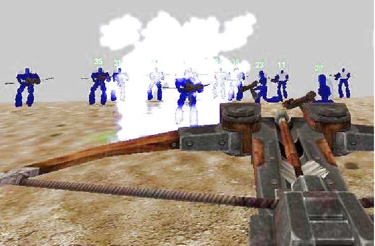
risk to human life of any real-world application, they make an excellent testbed for techniques in artificial
intelligence (Laird and van Lent 2000). Such techniques are also important for the video game industry:
They can potentially both increase the longevity of video games and decrease their production costs (Fogel
et al. 2004b).

    One of the most compelling yet least exploited technologies is machine learning. Thus, there is an
unexplored opportunity to make video games more interesting and realistic, and to build entirely new genres.
Such enhancements may have applications in education and training as well, changing the way people
interact with their computers.

    In the video game industry, the term non-player-character (NPC) refers to an autonomous computer-
controlled agent in the game. This paper focuses on training NPCs as intelligent agents, and the standard
AI term agents is therefore used to refer to them. The behavior of such agents in current games is often
repetitive and predictable. In most video games, simple scripts cannot learn or adapt to control the agents:
Opponents will always make the same moves and the game quickly becomes boring. Machine learning
could potentially keep video games interesting by allowing agents to change and adapt (Fogel et al. 2004b).
However, a major problem with learning in video games is that if behavior is allowed to change, the game
content becomes unpredictable. Agents might learn idiosyncratic behaviors or even not learn at all, making
the gaming experience unsatisfying. One way to avoid this problem is to train agents to perform complex
behaviors offline, and then freeze the results into the final, released version of the game. However, although
the game would be more interesting, the agents still could not adapt and change in response to the tactics of
particular players.

    If agents are to adapt and change in real-time, a powerful and reliable machine learning method is
needed. This paper describes such a method, a real-time enhancement of the NeuroEvolution of Augmenting
Topologies method (NEAT; Stanley and Miikkulainen 2002b, 2004a). NEAT evolves increasingly complex
neural networks, i.e. it complexifies. Real-time NEAT (rtNEAT) is able to complexify neural networks as
the game is played, making it possible for agents to evolve increasingly sophisticated behaviors in real
time. Thus, agent behavior improves visibly during gameplay. The aim is to show that machine learning is
indispensable for an interesting genre of video games, and to show how rtNEAT makes such an application
possible.

    In order to demonstrate the potential of rtNEAT, the Digital Media Collaboratory (DMC) at the Univer-
sity of Texas at Austin initiated, based on a proposal by Kenneth O. Stanley, the NeuroEvolving Robotic
Operatives (NERO) project in October of 2003 (http://nerogame.org). The idea was to create a

                                                      2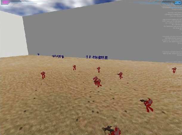
game in which learning is indispensable, in other words, without learning NERO could not exist as a game.
In NERO, the player takes the role of a trainer, teaching skills to a set of intelligent agents controlled by
rtNEAT. Thus, NERO is a powerful demonstration of how machine learning can open up new possibilities
in gaming and allow agents to adapt.

      NERO opens up new opportunities for interactive machine learning in entertainment, education, and
simulation. This paper describes rtNEAT and NERO, and reviews results from the first year of this ongoing
project. The next section presents a brief taxonomy of games that use learning, placing NERO in a broader
context. NEAT is then described, including how it was enhanced to create rtNEAT. The last sections describe
NERO and summarize the current status and performance of the game.

2 Related Work

Early successes in applying machine learning (ML) to board games have motivated more recent work in
live-action video games. For example, Samuel (1959) trained a computer to play checkers using a method
similar to temporal difference learning (Sutton 1988) in the first application of machine learning (ML) to
games. Since then, board games such as tic-tac-toe (Gardner 1962; Michie 1961), backgammon (Tesauro
and Sejnowski 1987), Go (Richards et al. 1997; Stanley and Miikkulainen 2004b), and Othello (Yoshioka
et al. 1998) have remained popular applications of ML (see Fürnkranz 2001 for a survey). A notable example
is Blondie24, which learned checkers by playing against itself without any built-in prior knowledge (Fogel
2001); also see Fogel et al. (2004a).

      Recently, interest has been growing in applying ML to video games (Fogel et al. 2004b; Laird and van
Lent 2000). For example, Fogel et al. (2004b) trained teams of tanks and robots to fight each other using
a competitive coevolution system designed for training video game agents. Others have trained agents to
fight in first- and third-person shooter games (Cole et al. 2004; Geisler 2002; Hong and Cho 2004). ML
techniques have also been applied to other video game genres from Pac-Man1 (Gallagher and Ryan 2003)
to strategy games (Bryant and Miikkulainen 2003; Revello and McCartney 2002; Yannakakis et al. 2004).
This section focuses on how machine learning can be applied to video games.

      From the human player’s perspective there are two types of learning in video games. In out-game
learning (OGL), game developers use ML techniques to pretrain agents that no longer learn after the game
is shipped. In contrast, in in-game learning (IGL), agents adapt as the player interacts with them in the game;
  1
      Pac-Man is a registered trademark of Namco, Ltd., of Tokyo, Japan.

                                                                3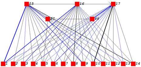
the player can either purposefully direct the learning process or the agents can adapt autonomously to the
player’s behavior. IGL is related to the broader field of interactive evolution, in which a user influences the
direction of evolution of e.g. art, music, or any other kind of phenotype (Parmee and Bonham 1999). Most
applications of ML to games have used OGL, though the distinction may be blurred from the researcher’s
perspective when online learning methods are used for OGL. However, the difference between OGL and IGL
is important to players and marketers, and ML researchers will frequently need to make a choice between
the two.

      In a Machine Learning Game (MLG), the player explicitly attempts to train agents as part of IGL. MLGs
are a new genre of video games that require powerful learning methods that can adapt during gameplay.
Although some conventional game designs include a “training” phase during which the player accumulates
resources or technologies in order to advance in levels, such games are not MLGs because the agents are not
actually adapting or learning.

      Prior examples in the MLG genre include the Tamagotchi virtual pet2 and the video “God game” Black
& White3 . In both games, the player shapes the behavior of game agents with positive or negative feedback.
It is also possible to train agents by human example during the game, as van Lent and Laird (2001) described
in their experiments with Quake II 4 . While these examples demonstrated that limited learning is possible in
a game, NERO is an entirely new kind of MLG; it uses a reinforcement learning method (neuroevolution) to
optimize a fitness function that is dynamically specified by the player while watching and interacting with
the learning agents. Thus agent behavior continues to improve as long as the game is played.

      A flexible and powerful ML method is needed to allow agents to adapt during gameplay. It is not enough
to simply script several key agent behaviors because adaptation would then be limited to the foresight of the
programmer who wrote the script, and agents would only be choosing from a limited menu of options.
Moreover, because agents need to learn online as the game is played, predetermined training targets are
usually not available, ruling out supervised techniques such as backpropagation (Rumelhart et al. 1986) and
decision tree learning (Utgoff 1989).

      Traditional reinforcement learning (RL) techniques such as Q-Learning (Watkins and Dayan 1992) and
Sarsa() with a Case-Based function approximator (SARSA-CABA; Santamaria et al. 1998) adapt in do-
mains with sparse feedback (Kaelbling et al. 1996; Sutton and Barto 1998; Watkins and Dayan 1992). These
  2
      Tamagotchi is a registered trademark of Bandai Co., Ltd., of Tokyo, Japan.
  3
      Black & White is a registered trademark of Lionhead Studios, Ltd., of Guildford, UK.
  4
      Quake II is a registered trademark of Id Software, Inc., of Mesquite, Texas.

                                                                  4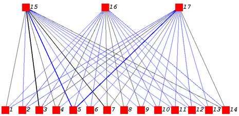
techniques learn to predict the long-term reward for taking actions in different states by exploring the state
space and keeping track of the results. While in principle it is possible to apply them to real-time learning
in video games, it would require significant work to overcome several common demands of video game
domains:

   1. Large state/action space. Since games usually have several different types of objects and characters
      and many different possible actions, the state/action space that RL must explore is extremely high
      dimensional. Dealing with high-dimensional spaces is a known challenge with RL in general (Sutton
      and Barto 1998), but in a real-time game there is the additional challenge of having to check the
      value of every possible action on every game tick for every agent in the game. Because traditional
      RL checks all such action values, the value estimator must execute several times (i.e. once for every
      possible action) for each agent in the game on every game tick. Action selection may thus incur a
      very large cost on the game engine, reducing the amount of computation available for the game itself.

   2. Diverse behaviors. Agents learning simultaneously in a simulated world should not all converge to
      the same behavior: A homogeneous population would make the game boring. Yet because many
      agents in video games have similar physical characteristics and are evaluated in a similar context,
      traditional RL techniques, many of which have convergence guarantees (Kaelbling et al. 1996), risk
      converging to largely homogeneous solution behaviors. Without explicitly maintaining diversity, such
      an outcome is likely.

   3. Consistent individual behaviors. RL depends on occasionally taking a random action in order to
      explore new behaviors. While this strategy works well in offline learning, players do not want to
      constantly see the same individual agent periodically making inexplicable and idiosyncratic moves
      relative to its usual policy.

   4. Fast adaptation and sophisticated behaviors. Because players do not want to wait hours for agents
      to adapt, it may be necessary to use a simple representation that can be learned quickly. However, a
      simple representation would limit the ability to learn sophisticated behaviors. Thus there is a trade-off
      between learning simple behaviors quickly and learning sophisticated behaviors more slowly, neither
      of which is desirable.

   5. Memory of past states. If agents remember past events, they can react more convincingly to the
      present situation. However, such memory requires keeping track of more than the current state, ruling

                                                      5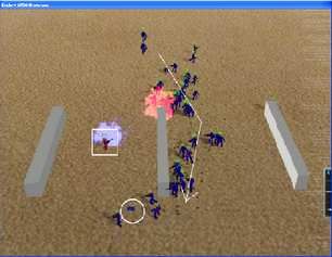
out traditional Markovian methods. While methods for partially observable Markov processes exist,
      significant challenges remain in scaling them up to real-world tasks (Gomez 2003).

   Neuroevolution (NE), i.e. the artificial evolution of neural networks using an evolutionary algorithm,
is an alternative RL technique that meets each of these demands naturally: (1) NE works well in high-
dimensional spaces (Gomez and Miikkulainen 2003); evolved agents do not need to check the value of more
than one action per game tick because agents are evolved to output only a single requested action per game
tick. (2) Diverse populations can be explicitly maintained through speciation (Stanley and Miikkulainen
2002b). (3) The behavior of an individual during its lifetime does not change because it always chooses
actions from the same network. (4) A representation of the solution can be evolved, allowing simple prac-
tical behaviors to be discovered quickly in the beginning and complexified later (Stanley and Miikkulainen
2004a). (5) Recurrent neural networks can be evolved that implement and utilize effective memory struc-
tures; for example, NE has been used to evolve motor-control skills similar to those in continuous-state
games in many challenging non-Markovian domains (Aharonov-Barki et al. 2001; Floriano and Mondada
1994; Fogel 2001; Gomez and Miikkulainen 1998, 1999, 2003; Gruau et al. 1996; Harvey 1993; Moriarty
and Miikkulainen 1996b; Nolfi et al. 1994; Potter et al. 1995; Stanley and Miikkulainen 2004a; Whitley
et al. 1993). In addition to these five demands, neural networks also make good controllers for video game
agents because they can compute arbitrarily complex functions, can both learn and perform in the presence
of noisy inputs, and generalize their behavior to previously unseen inputs (Cybenko 1989; Siegelmann and
Sontag 1994). Thus, NE is a good match for video games.

   There is a large variety of NE algorithms (Yao 1999). While some evolve only the connection weight
values of fixed-topology networks (Gomez and Miikkulainen 1999; Moriarty and Miikkulainen 1996a; Sar-
avanan and Fogel 1995; Wieland 1991), others evolve both weights and network topology simultaneously
(Angeline et al. 1993; Bongard and Pfeifer 2001; Braun and Weisbrod 1993; Dasgupta and McGregor 1992;
Gruau et al. 1996; Hornby and Pollack 2002; Krishnan and Ciesielski 1994; Lee and Kim 1996; Mandischer
1993; Maniezzo 1994; Opitz and Shavlik 1997; Pujol and Poli 1997; Yao and Liu 1996; Zhang and Muh-
lenbein 1993). Topology and Weight Evolving Artificial Neural Networks (TWEANNs) have the advantage
that the correct topology need not be known prior to evolution. Among TWEANNs, NEAT is unique in that
it begins evolution with a population of minimal networks and adds nodes and connections to them over
generations, allowing complex problems to be solved gradually based on simple ones.

   Our research group has been applying NE to gameplay for about a decade. Using this approach, sev-
eral NE algorithms have been applied to board games (Moriarty and Miikkulainen 1993; Moriarty 1997;

                                                    6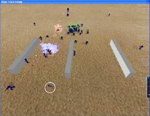
Richards et al. 1997; Stanley and Miikkulainen 2004b). In Othello, NE discovered the mobility strategy
only a few years after its invention by humans (Moriarty and Miikkulainen 1993). Recent work has focused
on higher-level strategies and real-time adaptation, which are needed for success in both continuous and
discrete multi-agent games (Agogino et al. 2000; Bryant and Miikkulainen 2003; Stanley and Miikkulainen
2004a). Using such techniques, relatively simple ANN controllers can be trained in games and game-like
environments to produce convincing purposeful and intelligent behavior (Agogino et al. 2000; Gomez and
Miikkulainen 1998; Moriarty and Miikkulainen 1995a,b, 1996b; Richards et al. 1997; Stanley and Miikku-
lainen 2004a).

    The current challenge is to achieve evolution in real time, as the game is played. If agents could be
evolved in a smooth cycle of replacement, the player could interact with evolution during the game and
the many benefits of NE would be available to the video gaming community. This paper introduces such
a real-time NE technique, rtNEAT, which is applied to the NERO multi-agent continuous-state MLG. In
NERO, agents must master both motor control and higher-level strategy to win the game. The player acts
as a trainer, teaching a team of virtual robots the skills they need to survive. The next section reviews the
NEAT neuroevolution method, and Section 4 how it can be enhanced to produce rtNEAT.

3 NeuroEvolution of Augmenting Topologies (NEAT)

The rtNEAT method is based on NEAT, a technique for evolving neural networks for complex reinforcement
learning tasks using an evolutionary algorithm (EA). NEAT combines the usual search for the appropriate
network weights with complexification of the network structure, allowing the behavior of evolved neural
networks to become increasingly sophisticated over generations.

    The NEAT method consists of solutions to three fundamental challenges in evolving neural network
topology: (1) What kind of genetic representation would allow disparate topologies to cross over in a mean-
ingful way? The solution is to use historical markings to line up genes with the same origin. (2) How can
topological innovation that needs a few generations to optimize be protected so that it does not disappear
from the population prematurely? The solution is to separate each innovation into a different species. (3)
How can topologies be minimized throughout evolution so the most efficient solutions will be discovered?
The solution is to start from a minimal structure and add nodes and connections incrementally. This section
explains how each of these solutions is implemented in NEAT, using the genetic encoding described in the
first subsection.

                                                     7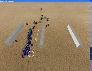
Genome (Genotype)

           Node    Node 1 Node 2 Node 3 Node 4 Node 5
           Genes   Input      Input   Input       Output Hidden

           Connect. Innov 1      Innov 2          Innov 3     Innov 4   Innov 5   Innov 6   Innov 11
           Genes In 1            In 2             In 3        In 2      In 5      In 1      In 4
                   Out 4         Out 4            Out 4       Out 5     Out 4     Out 5     Out 5
                   Weight 0.7 Weight−0.5 Weight 0.5 Weight 0.2 Weight 0.4 Weight 0.6 Weight 0.6
                   Enabled       DISABLED         Enabled     Enabled   Enabled   Enabled   Enabled

                                                          4
                    Network (Phenotype)
                                                          5

                                              1          2     3

Figure 1: A NEAT genotype to phenotype mapping example. A genotype is depicted that produces the shown
phenotype. There are three input nodes, one hidden node, one output node, and seven connection definitions, one
of which is recurrent. The second gene is disabled, so the connection that it specifies (between nodes 2 and 4) is
not expressed in the phenotype. The genotype can have arbitrary length, and thereby represent arbitrarily complex
networks. Innovation numbers, which allow NEAT to identify which genes match up between different genomes, are
shown on top of each gene. This encoding is efficient and allows changing the network structure during evolution.

3.1 Genetic Encoding

Evolving structure requires a flexible genetic encoding. In order to allow structures to complexify, their
representations must be dynamic and expandable. Each genome in NEAT includes a list of connection
genes, each of which refers to two node genes being connected (Figure 1). Each connection gene specifies
the in-node, the out-node, the weight of the connection, whether or not the connection gene is expressed (an
enable bit), and an innovation number, which allows finding corresponding genes during crossover.

    Mutation in NEAT can change both connection weights and network structures. Connection weights
mutate as in any NE system, with each connection either perturbed or not. Structural mutations, which form
the basis of complexification, occur in two ways (Figure 2). Each mutation expands the size of the genome
by adding genes. In the add connection mutation, a single new connection gene is added connecting two
previously unconnected nodes. In the add node mutation, an existing connection is split and the new node
placed where the old connection used to be. The old connection is disabled and two new connections added
to the genome. The connection between the first node in the chain and the new node is given a weight of
one, and the connection between the new node and the last node in the chain is given the same weight as the
connection being split. Splitting the connection in this way introduces a nonlinearity (the sigmoid function)

                                                              8
Add Connection Mutation
1 2 3 4 5 6 1 2 3 4 5 6 7
1−>4 2−>4 3−>4 2−>5 5−>4 1−>5 1−>4 2−>4 3−>4 2−>5 5−>4 1−>5 3−>5
DIS DIS
4 4
5 5
1 2 3 1 2 3
Add Node Mutation
1 2 3 4 5 6 1 2 3 4 5 6 8 9
1−>4 2−>4 3−>4 2−>5 5−>4 1−>5 1−>4 2−>4 3−>4 2−>5 5−>4 1−>5 3−>6 6−>4
DIS DIS DIS
4 4
5 5
6
1 2 3 1 2 3
Figure 2: The two types of structural mutation in NEAT. In each genome, the innovation number is shown on
top, the two nodes connected by the gene in the middle, and the “disabled” symbol at the bottom; the weights and
the node genes are not shown for simplicity. A new connection or a new node is added to the network by adding
connection genes to the genome. Assuming the node is added after the connection, the genes would be assigned
innovation numbers 7, 8, and 9, as the figure illustrates. NEAT can keep an implicit history of the origin of every gene
in the population, allowing matching genes to be identified even in different genome structures.
where there was none before. This nonlinearity changes the function only slightly, and the new node is
immediately integrated into the network. Old behaviors encoded in the preexisting network structure are not
destroyed and remain qualitatively the same, while the new structure provides an opportunity to elaborate
on these original behaviors.
Through mutation, the genomes in NEAT will gradually get larger. Genomes of varying sizes will
result, sometimes with different connections at the same positions. Any crossover operator must be able
to recombine networks with differing topologies, which can be difficult (Radcliffe 1993). The next section
explains how NEAT addresses this problem.
3.2 Tracking Genes through Historical Markings
The historical origin of each gene can be used to determine exactly which genes match up between any indi-
viduals in the population. Two genes with the same historical origin represent the same structure (although
possibly with different weights), since they were both derived from the same ancestral gene at some point
in the past. Thus, in order to properly align and recombine any two disparate topologies in the population
the system only needs to keep track of the historical origin of each gene.
9Tracking the historical origins requires very little computation. Whenever a new gene appears (through
structural mutation), a global innovation number is incremented and assigned to that gene. The innovation
numbers thus represent a chronology of every gene in the population. As an example, say the two mutations
in Figure 2 occurred one after another. The new connection gene created in the first mutation is assigned the
number 7, and the two new connection genes added during the new node mutation are assigned the numbers
8 and 9. In the future, whenever these genomes cross over, the offspring will inherit the same innovation
numbers on each gene. Thus, the historical origin of every gene is known throughout evolution.
A possible problem is that the same structural innovation will receive different innovation numbers in
the same generation if it occurs by chance more than once. However, by keeping a list of the innovations
that occurred in the current generation, it is possible to ensure that when the same structure arises more than
once through independent mutations in the same generation, each identical mutation is assigned the same
innovation number.
Through innovation numbers, the system now knows exactly which genes match up with which (Figure
3). Genes that do not match are either disjoint or excess, depending on whether they occur within or outside
the range of the other parent’s innovation numbers.
When crossing over, the genes with the same innovation numbers are lined up. The offspring is then
formed in one of two ways: In uniform crossover, matching genes are randomly chosen for the offspring
genome. In blended crossover (Wright 1991), the connection weights of matching genes are averaged. These
two types of crossover were found to be most effective in NEAT in extensive testing compared to one-point
crossover.
The disjoint and excess genes are inherited from the more fit parent, or if they are equally fit, from both
parents. Disabled genes have a chance of being reenabled during crossover, allowing networks to make use
of older genes once again.
Historical markings allow NEAT to perform crossover without analyzing topologies. Genomes of differ-
ent organizations and sizes stay compatible throughout evolution, and the variable-length genome problem
is essentially avoided. This methodology allows NEAT to complexify structure while different networks
still remain compatible.
However, it turns out that it is difficult for a population of varying topologies to support new innovations
that add structure to existing networks. Because smaller structures optimize faster than larger structures,
and adding nodes and connections usually initially decreases the fitness of the network, recently augmented
structures have little hope of surviving more than one generation even though the innovations they represent
10Parent1 Parent2
1 2 3 4 5 8 1 2 3 4 5 6 7 9 10
1−>4 2−>4 3−>4 2−>5 5−>4 1−>5 1−>4 2−>4 3−>4 2−>5 5−>4 5−>6 6−>4 3−>5 1−>6
DIS DIS DIS
4 4
5 6
5
1 2 3 1 2 3
disjoint
1 2 3 4 5 8
Parent1 1−>4 2−>4 3−>4 2−>5 5−>4 1−>5
DIS
1 2 3 4 5 6 7 9 10
Parent2 1−>4 2−>4 3−>4 2−>5 5−>4 5−>6 6−>4 3−>5 1−>6
DIS DIS
disjoint disjoint excess excess
1 2 3 4 5 6 7 8 9 10
Offspring 1−>4 2−>4 3−>4 2−>5 5−>4 5−>6 6−>4 1−>5 3−>5 1−>6
DIS DIS
4
6
5
1 2 3
Figure 3: Matching up genomes for different network topologies using innovation numbers. Although Parent
1 and Parent 2 look different, their innovation numbers (shown at the top of each gene) indicate that several of their
genes match up even without topological analysis. A new structure that combines the overlapping parts of the two
parents as well as their different parts can be created in crossover. In this case, the two parents are assumed to have
equal fitness, and therefore the offspring inherits all such genes from both parents. Otherwise these genes would be
inherited from the more fit parent only. The disabled genes may become enabled again in future generations: There
is a preset chance that an inherited gene is enabled if it is disabled in either parent. By matching up genes in this
way, it is possible to determine the best alignment for crossover between any two arbitrary network topologies in the
population.
might be crucial towards solving the task in the long run. The solution is to protect innovation by speciating
the population, as explained in the next section.
3.3 Protecting Innovation through Speciation
NEAT speciates the population so that individuals compete primarily within their own niches instead of
with the population at large. This way, topological innovations are protected and have time to optimize their
structure before they have to compete with other niches in the population. Protecting innovation through
speciation follows the philosophy that new ideas must be given time to reach their potential before they are
eliminated. A secondary benefit of speciation is that is prevents bloating of genomes: Species with smaller
11genomes survive as long as their fitness is competitive, ensuring that small networks are not replaced by
larger ones unnecessarily.
Historical markings make it possible for the system to divide the population into species based on how
similar they are topologically (figure 4). The distance Æ between two network encodings can be measured
as a linear combination of the number of excess (E ) and disjoint (D ) genes, as well as the average weight
differences of matching genes (W ):
1E 2D
Æ=
N
+
N
+ 3 W: (1)
The coefficients 1 , 2 , and 3 adjust the importance of the three factors, and the factor N , the number
of genes in the larger genome, normalizes for genome size (N can be set to one unless both genomes are
excessively large). Genomes are tested one at a time; if a genome’s distance to a randomly chosen member
of the species is less than Æt , a compatibility threshold, the genome is placed into this species.
If a genome is not compatible with any existing species, a new species is created. The problem of
choosing the best value for Æt can be avoided by making Æt dynamic; that is, given a target number of
species, the system can slightly raise Æt if there are too many species, and lower Æt if there are too few. Each
genome is placed into the first species from the previous generation where this condition is satisfied, so that
no genome is in more than one species. Keeping the same set of species from one generation to the next
allows NEAT to remove stagnant species, i.e. species that have not improved for several generations.
As the reproduction mechanism, NEAT uses explicit fitness sharing (Goldberg and Richardson 1987),
where organisms in the same species must share the fitness of their niche. Thus, a species cannot afford to
become too big even if many of its organisms perform well. Therefore, any one species is unlikely to take
over the entire population, which is crucial for speciated evolution to support a variety of topologies. The
adjusted fitness fi0 for organism i is calculated according to its distance Æ from every other organism j in the
population:
fi0 = Pnj=1 fi
sh(Æ (i; j ))
: (2)
sh is set to 0 when distance Æ (i; j ) is above the threshold Æt ; otherwise, sh(Æ (i; j ))
P
The sharing function is
set to 1 (Spears 1995). Thus, nj=1 sh(Æ (i; j )) reduces to the number of organisms in the same species as
organism i. This reduction is natural since species are already clustered by compatibility using the threshold
Æt . Every species is assigned a potentially different number of offspring in proportion to the sum of adjusted
fitnesses fi0 of its member organisms.
The net effect of fitness sharing in NEAT can be summarized as follows. Let Fk be the average fitness of
12The Genome Loop:
Take the next genome g from population P
The Species Loop:
If all species in S have been checked,
create new species snew and place g in it
Else
Get the next species s from S
If g is compatible with s, add g to s
If g has not been placed,
continue the Species Loop
Else exit the Species Loop
If not all genomes in G have been placed,
continue the Genome Loop
Else exit the Genome Loop
Figure 4: Procedure for speciating the population in NEAT. The speciation procedure consists of two nested loops
that allocate the entire population into species. Figure 6 shows how it can be done continuously in real time.
species k and jP j be the size of the population. Let F tot =
Pk Fk be the total of all species fitness averages.
The number of offspring nk allotted to species k is:
Fk
nk =
F tot
jP j: (3)
Species reproduce by first eliminating the lowest performing members from the population. The entire
population is then replaced by the offspring of the remaining individuals in each species.
The main effect of speciating the population is that structural innovation is protected. The final goal
of the system, then, is to perform the search for a solution as efficiently as possible. This goal is achieved
through complexification from a simple starting structure, as detailed in the next section.
3.4 Minimizing Dimensionality through Complexification
Other systems that evolve network topologies and weights begin evolution with a population of random
topologies (Angeline et al. 1993; Gruau et al. 1996; Yao 1999; Zhang and Muhlenbein 1993). In contrast,
NEAT begins with a uniform population of simple networks with no hidden nodes, differing only in their
13initial random weights. Speciation protects new innovations, allowing diverse topologies to gradually accu-
mulate over evolution. Thus, NEAT can start minimally, and grow the necessary structure over generations.
New structures are introduced incrementally as structural mutations occur, and only those structures
survive that are found to be useful through fitness evaluations. In this way, NEAT searches through a
minimal number of weight dimensions, significantly reducing the number of generations necessary to find
a solution, and ensuring that networks become no more complex than necessary. This gradual increase in
complexity over generations is similar to complexification in biology (Amores et al. 1998; Carroll 1995;
Force et al. 1999; Martin 1999). In effect, then, NEAT searches for the optimal topology by incrementally
complexifying existing structure.
3.5 NEAT Performance
In previous work, each of the three main components of NEAT (i.e. historical markings, speciation, and
starting from minimal structure) were experimentally ablated in order to determine how they contribute to
performance (Stanley and Miikkulainen 2002b). The ablation study demonstrated that all three components
are interdependent and necessary to make NEAT work.
The NEAT approach is also highly effective: NEAT outperforms other neuroevolution (NE) methods,
e.g. on the benchmark double pole balancing task (Stanley and Miikkulainen 2002a,b). In addition, because
NEAT starts with simple networks and expands the search space only when beneficial, it is able to find
significantly more complex controllers than fixed-topology evolution (Stanley and Miikkulainen 2004a).
These properties make NEAT an attractive method for evolving neural networks in complex tasks such as
video games. The next section explains how NEAT can be enhanced to work in real time.
4 Real-time NEAT (rtNEAT)
Like most EAs, NEAT was originally designed to run offline. Individuals are evaluated one or two at a time,
and after the whole population has been tested, a new population is created to form the next generation. In
other words, in a normal EA it is not possible for a human to interact with the evolving agents while they
are evolving. This section describes how NEAT can be modified to make it possible for players to interact
with evolving agents in real time.
142 high−fitness agents
1 low−fitness agent X
Cross over
Mutate
New agent
Figure 5: The main replacement cycle in rtNEAT. NE agents (represented as small circles with an arrow indicating
their direction) are depicted playing a game in the large box. Every few ticks, two high-fitness agents are selected to
produce an offspring that replaces another of lower fitness. This cycle of replacement operates continually throughout
the game, creating a constant turnover of new behaviors that is largely invisible to the player.
4.1 Motivation
At each generation, NEAT evaluates one complete generation of individuals before creating the next gener-
ation. Real-time neuroevolution is based on the observation that in a video game, the entire population of
agents plays at the same time. Therefore, fitness statistics are collected constantly as the game is played,
and the agents could in principle be evolved continuously as well.
The central question is how the agents can be replaced continuously so that offspring can be evaluated.
Replacing the entire population together on each generation would look incongruous to the player since
everyone’s behavior would change at once. In addition, behaviors would remain static during the large gaps
of time between generations.
The alternative is to replace a single individual every few game ticks as is done in some evolutionary
strategy algorithms (Beyer and Paul Schwefel 2002). One of the worst individuals is removed and replaced
with a child of parents chosen from among the best. If this cycle of removal and replacement happens
continually throughout the game (figure 5), evolution is largely invisible to the player.
Real-time evolution using continuous replacement was first implemented using conventional neuroevo-
lution before NEAT was developed and applied to a Warcraft II5 -like video game (Agogino et al. 2000). A
5
Warcraft II is a registered trademark of Blizzard Entertainment, of Irvine, California.
15The rtNEAT Loop:
Calculate the adjusted fitness of all current
individuals in the population
Remove the agent with the worst adjusted
fitness from the population provided one has
been alive sufficiently long so that it has
been properly evaluated.
Re-estimate the average fitness F for all
species
Choose a parent species to create the new
offspring
Adjust Æt dynamically and reassign all agents
to species
Place the new agent in the world
Figure 6: Operations performed every n ticks by rtNEAT. These operations allow evolution to proceed continu-
ously, with the same dynamics as in original NEAT.
similar real-time conventional neuroevolution system was later demonstrated by Yannakakis et al. (2004)
in a predator/prey domain. However, conventional neuroevolution is not sufficiently powerful to meet the
demands of modern video games. In contrast, a real-time version of NEAT offers the advantages of NEAT:
Agent neural networks can become increasingly sophisticated and complex during gameplay. The challenge
is to preserve the usual dynamics of NEAT, namely protection of innovation through speciation and com-
plexification. While original NEAT assigns offspring to species en masse for each new generation, rtNEAT
cannot do the same because it only produces one new offspring at a time. Therefore, the reproduction cycle
must be modified to allow rtNEAT to speciate in real-time. This cycle constitutes the core of rtNEAT.
4.2 The rtNEAT Algorithm
In the rtNEAT algorithm, a sequence of operations aimed at introducing a new agent into the population are
repeated at a regular time interval, i.e. every n ticks of the game clock (figure 6). The new agent will replace a
poorly performing individual in the population. The algorithm preserves the speciation dynamics of original
NEAT by probabilistically choosing parents to form the offspring and carefully selecting individuals to
replace. Each of the steps in figure 6 is discussed in more detail below.
164.2.1 Calculating adjusted fitness
Let fi be the original fitness of individual i. Fitness sharing adjusts it to jfSij , where jS j is the number of
individuals in the species (Section 3.3).
4.2.2 Removing the worst agent
The goal of this step is to remove a poorly performing agent from the game, hopefully to be replaced by
something better. The agent must be chosen carefully to preserve speciation dynamics. If the agent with
the worst unadjusted fitness were chosen, fitness sharing could no longer protect innovation because new
topologies would be removed as soon as they appear. Thus, the agent with the worst adjusted fitness should
be removed, since adjusted fitness takes into account species size, so that new, smaller species are not
removed as soon as they appear.
It is also important that agents are evaluated sufficiently before they are considered for removal. In
original NEAT, networks are generally all evaluated for the same amount of time. However, in rtNEAT,
new agents are constantly being born, meaning different agents have been around for different lengths of
time. Therefore, rtNEAT only removes agents who have played for more than the minimum amount of time
m. This parameter is set experimentally, by observing how much time is required for an agent to execute a
substantial behavior in the game.
4.2.3 Re-estimating F
Assuming there was an agent old enough to be removed, its species now has one less member and therefore
its average fitness F has likely changed. It is important to keep F up-to-date because F is used in choosing
the parent species in the next step. Therefore, F needs to be calculated in each step.
4.2.4 Creating offspring
Because only one offspring is created at a time, equation 3 does not apply to rtNEAT. However, its effect can
be approximated by choosing the parent species probabilistically based on the same relationship of adjusted
fitnesses:
Fk
P r (Sk ) = : (4)
F tot
17In other words, the probability of choosing a given parent species is proportional to its average fitness
compared to the total of all species’ average fitnesses. Thus, over the long run, the expected number of
offspring for each species is proportional to nk , preserving the speciation dynamics of original NEAT. A
single new offspring is created by recombining two individuals from the parent species.
4.2.5 Reassigning Agents to Species
As was discussed in Section 3.3, the dynamic compatibility threshold Æt keeps the number of species rela-
tively stable throughout evolution. Such stability is particularly important in a real-time video game since
the population may need to be consistently small to accommodate CPU resources dedicated to graphical
processing.
In original NEAT, Æt can be adjusted before the next generation is created. In rtNEAT, changing Æt alone
is not sufficient because most of the population would still remain in their current species. Instead, the
entire population must be reassigned to the existing species based on the new Æt . As in original NEAT, if a
network does not get assigned to any of the existing species, a new species is created with that network as its
representative. Depending on the specific game, species do not need to be reorganized at every replacement.
The number of ticks between adjustments can be chosen by the game designer based on how rapidly the
species evolve. In NERO, evolution progresses rather quickly, and the reorganization is done every five
replacements.
4.2.6 Replacing the old agent with the new one
Since an individual was removed in step 4.2.2, the new offspring needs to replace it. How agents are replaced
depends on the game. In some games (such as NERO), the neural network can be removed from a body
and replaced without doing anything to the body. In others, the body may have been destroyed and need to
be replaced as well. The rtNEAT algorithm can work with any of these schemes as long as an old neural
network gets replaced with a new one.
4.3 Running the algorithm
The 6-step rtNEAT algorithm is necessary to approximate original NEAT in real-time. However, there is
one remaining issue. The entire loop should be performed at regular intervals, every n ticks: How should n
be chosen?
18If agents are replaced too frequently, they do not live long enough to reach the minimum time m to be
evaluated. On the other hand, if agents are replaced too infrequently, evolution slows down to a pace that
the player no longer enjoys.
Interestingly, the appropriate frequency can be determined through a principled approach. Let I be the
fraction of the population that is too young and therefore cannot be replaced. As before, n is the number
of ticks between replacements, m is the minimum time alive, and jP j is the population size. A law of
eligibility can be formulated that specifies what fraction of the population can be expected to be ineligible
once evolution reaches a steady state (i.e. after the first few time steps when no one is eligible):
m
I =
jP jn : (5)
According to Equation 5, the larger the population and the more time between replacements, the lower the
fraction of ineligible agents. This principle makes sense since in a larger population it takes more time
to replace the entire population. Also, the more time passes between replacements, the more time the
population has to age, and hence fewer are ineligible. On the other hand, the larger the minimum age, the
more are below it, and fewer agents are eligible.
It is also helpful to think of m
n as the number of individuals that must be ineligible at any time; over the
course of m ticks, an agent is replaced every n ticks, and all the new agents that appear over m ticks will
remain ineligible for that duration since they cannot have been around for over m ticks. For example, if jP j
is 50, m is 500, and n is 20, 50% of the population would be ineligible at any one time.
Based on the law of eligibility, rtNEAT can decide on its own how many ticks n should lapse between
replacements for a preferred level of ineligibility, specific population size, and minimum time between
replacements:
m
n=
jP jI : (6)
It is best to let the user choose I because in general it is most critical to performance; if too much of the
population is ineligible at one time, the mating pool is not sufficiently large. Equation 6 then allows rtNEAT
to determine the appropriate number of ticks between replacements. In NERO, 50% of the population
remains eligible using this technique.
By performing the right operations every n ticks, choosing the right individual to replace and replacing
it with an offspring of a carefully chosen species, rtNEAT is able to replicate the dynamics of NEAT in
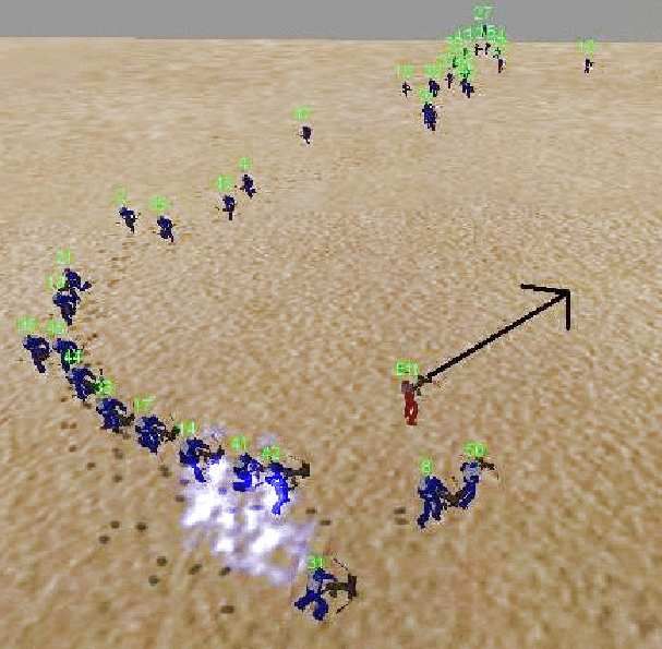
19Scenario 1: Enemy Turret Scenario 2: 2 Enemy Turrets Scenario 3: Mobile Turrets & Walls Battle
Figure 7: A turret training sequence. The figure depicts a sequence of increasingly difficult and complicated
training exercises in which the agents attempt to attack turrets without getting hit. In the first exercise there is only a
single turret but more turrets are added by the player as the team improves. Eventually walls are added and the turrets
are given wheels so they can move. Finally, after the team has mastered the hardest exercises, it is deployed in a real
battle against another team.
real-time. Thus, it is now possible to deploy NEAT in a real video game and interact with complexifying
agents as they evolve. The next section describes such a game.
5 NeuroEvolving Robotic Operatives (NERO)
NERO is representative of a new MLG genre that is only possible through machine learning. The idea is
to put the player in the role of a trainer or a drill instructor who teaches a team of agents by designing a
curriculum. Of course, for the player to be able to teach agents, the agents must be able to learn; rtNEAT is
the learning algorithm that makes NERO possible.
In NERO, the learning agents are simulated robots, and the goal is to train a team of these agents for
military combat. The agents begin the game with no skills and only the ability to learn. In order to prepare
for combat, the player must design a sequence of training exercises and goals. Ideally, the exercises are
increasingly difficult so that the team can begin by learning basic skills and then gradually build on them
(figure 7). When the player is satisfied that the team is well prepared, the team is deployed in a battle against
another team trained by another player, making for a captivating and exciting culmination of training. The
challenge is to anticipate the kinds of skills that might be necessary for battle and build training exercises to
hone those skills. The next two sections explain how the agents are trained in NERO and how they fight an
opposing team in battle.
20(a) Objects (b) Sliders
Figure 8: Setting up training scenarios. These NERO screenshots show examples of items that the player can place
on the field, and sliders used to control the agents’ behavior. (a) Three types of enemies are shown from left to right:
a rover that runs in a preset pattern, a static enemy that stands in a single location, and a rotating turret with a gun. To
the right of the turret is a flag that NERO agents can learn to approach or avoid. Behind these objects is a wall. The
player can place any number and any configuration of these items on the training field. (b) Interactive sliders specify
the player’s preference for the behavior the team should try to optimize. For example the “E” icon means “approach
enemy,” and the descending bar above it specifies that the player wants to punish agents that approach the enemy.
The crosshair icon represents “hit target,” which is being rewarded. The sliders are used to specify coefficients for the
corresponding components of the fitness function that NEAT optimizes. Through placing items on the field and setting
sliders, the player creates training scenarios where learning takes place.
5.1 Training Mode
The player sets up training exercises by placing objects on the field and specifying goals through several
sliders (figure 8). The objects include static enemies, enemy turrets, rovers (i.e. turrets that move), flags,
and walls. To the player, the sliders serve as an interface for describing ideal behavior. To rtNEAT, they
represent coefficients for fitness components. For example, the sliders specify how much to reward or punish
approaching enemies, hitting targets, getting hit, following friends, dispersing, etc. Each individual fitness
component is normalized to a Z-score (i.e. the number of standard deviations from the mean) so that each
fitness component is measured on the same scale. Fitness is computed as the sum of all these components
multiplied by their slider levels, which can be positive or negative. Thus, the player has a natural interface
for setting up a training exercise and specifying desired behavior.
Agents have several types of sensors. Although NERO programmers frequently experiment with new
sensor configurations, the standard sensors include enemy radars, an “on target” sensor, object rangefinders,
and line-of-fire sensors. Figure 9 shows a neural network with the standard set of sensors and outputs, and
figure 10 describes how the sensors function.
Training mode is designed to allow the player to set up a training scenario on the field where the agents
can continually be evaluated while the worst agent’s neural network is replaced every few ticks. Thus,
training must provide a standard way for agents to appear on the field in such a way that every agent has
an equal chance to prove its worth. To meet this goal, the agents spawn from a designated area of the field
21Left/Right Forward/Back Fire
Evolved Topology
Bias
Enemy Radars On Object Rangefiners Enemy
Target LOF
Sensors
Figure 9: NERO input sensors and action outputs. Each NERO agent can see enemies, determine whether an
enemy is currently in its line of fire, detect objects and walls, and see the direction the enemy is firing. Its outputs
specify the direction of movement and whether or not to fire. This configuration has been used to evolve varied and
complex behaviors; other variations work as well and the standard set of sensors can easily be changed in NERO.
(a) Enemy Radars (b) Rangefinders
(c) On-Target Sensor (d) Line-of-fire sensors
Figure 10: NERO sensor design. All NERO sensors are egocentric, i.e. they tell where the objects are from
the agent’s perspective. (a) Several enemy radar sensors divide the 360 degrees around the agent into slices. Each
slice activates a sensor in proportion to how close an enemy is within that slice. If there is more than one enemy
in it, their activations are summed. (b) Rangefinders project rays at several angles from the agent. The distance
the ray travels before it hits an object is returned as the value of the sensor. Rangefinders are useful for detecting
long contiguous objects whereas radars are appropriate for relatively small, discrete objects. (c) The on-target sensor
returns full activation only if a ray projected along the front heading of the agents hits an enemy. This sensor tells
the agent whether it should attempt to shoot. (d) The line of fire sensors detect where a bullet stream from the closest
enemy is heading. Thus, these sensors can be used to avoid fire. They work by computing where the line of fire
intersects rays projecting from the agent, giving a sense of the bullet’s path. Together, these four kinds of sensors
provide sufficient information for agents to learn successful behaviors for battle. Other sensors can be added based on
the same structures, such as radars for detecting a flag or friendly agents on the same team.
22called the factory. Each agent is allowed a limited time on the field during which its fitness is assessed.
When their time on the field expires, agents are transported back to the factory, where they begin another
evaluation. Neural networks are only replaced in agents that have been put back in the factory. The factory
ensures that a new neural network cannot get lucky (or unlucky) by appearing in an agent that happens to be
standing in an advantageous (or difficult) position: All evaluations begin consistently in the factory.
The fitness of agents that survive more than one deployment on the field is updated through a diminishing
average that gradually forgets deployments from the distant past. A true average is first computed over the
first few trials (e.g. 2) and a continuous leaky average (similar to TD(0) reinforcement learning update
(Sutton and Barto 1998)) is maintained thereafter:
st ft
ft+1 = ft + (7)
r
where ft is the current fitness, st is the score from the current evaluation, and r controls the rate of forgetting.
The lower r is set, the sooner recent evaluations are forgotten. In this process, older agents have more reliable
fitness measures since they are averaged over more deployments than younger agents, but their fitness does
not become out of date.
Training begins by deploying 50 agents on the field. Each agent is controlled by a neural network with
random connection weights and no hidden nodes, which is the usual starting configuration for NEAT (see
Appendix A for a complete description of the rtNEAT parameters used in NERO). As the neural networks
are replaced in real-time, behavior improves dramatically, and agents eventually learn to perform the task
the player sets up. When the player decides that performance has reached a satisfactory level, he or she can
save the team in a file. Saved teams can be reloaded for further training in different scenarios, or they can
be loaded into battle mode. In battle, they face off against teams trained by an opponent player, as will be
described next.
5.2 Battle Mode
In battle mode, the player discovers how well the training worked out. Each player assembles a battle team
of 20 agents from as many different trained teams as desired. For example, perhaps some agents were trained
for close combat while others were trained to stay far away and avoid fire. A player may choose to compose
a heterogeneous team from both training sessions, and deploy it in battle.
Battle mode is designed to run over a server so that two players can watch the battle from separate
23(a) (b) (c)
Figure 11: Battlefield configurations. A range of possible configurations from an open pen (a) to a maze-like
environment (c) can be created for NERO. Players can construct their own battlefield configurations and train for
them. The basic configuration, which is used in Section 6, is the empty pen surrounded by four bounding walls, as
shown in (a).
terminals on the Internet. The battle begins with the two teams arrayed on opposite sides of the field. When
one player presses a “go” button, the neural networks obtain control of their agents and perform according
to their training. Unlike in training, where being shot does not lead to an agent body being damaged, the
agents are actually destroyed after being shot several times (currently five) in battle. The battle ends when
one team is completely eliminated. In some cases, the only surviving agents may insist on avoiding each
other, in which case action ceases before one side is completely destroyed. In that case, the winner is the
team with the most agents left standing.
The basic battlefield configuration is an empty pen surrounded by four bounding walls, although it is
possible to compete on a more complex field with walls or other obstacles (figure 11). In the experiments
described in this paper, the battlefield was the basic pen, and the agents were trained specifically for this
environment. The next section gives examples of actual NERO training and battle sessions.
6 Playing NERO
Behavior can be evolved very quickly in NERO, fast enough so that the player can be watching and inter-
acting with the system in real time. The game engine Torque, licensed from GarageGames
(http://www.garagegames.com/), drives NERO’s simulated physics and graphics. An important
property of the Torque engine is that its physics is slightly nondeterministic, so that the same game is never
played twice. In addition, Torque makes it possible for the player to take control of enemy robots using a
joystick, an option that can be useful in training.
24You can also read