Numerical Inside View of Hypermassive Remnant Models for GW170817
←
→
Page content transcription
If your browser does not render page correctly, please read the page content below
Numerical Inside View of Hypermassive Remnant Models for GW170817

                                                                                                      W. Kastaun1, 2 and F. Ohme1, 2
                                                        1
                                                            Max Planck Institute for Gravitational Physics (Albert Einstein Institute), Callinstr. 38, D-30167 Hannover, Germany
                                                                                      2
                                                                                        Leibniz Universität Hannover, D-30167 Hannover, Germany
                                                                  The first multimessenger observation attributed to a merging neutron star binary provided an enormous
                                                               amount of observational data. Unlocking the full potential of this data requires a better understanding of the
                                                               merger process and the early post-merger phase, which are crucial for the later evolution that eventually leads to
                                                               observable counterparts. In this work, we perform standard hydrodynamical numerical simulations of a system
                                                               compatible with GW170817. We focus on a single equation of state (EOS) and two mass ratios, while neglect-
                                                               ing magnetic fields and neutrino radiation. We then apply newly developed postprocessing and visualization
                                                               techniques to the results obtained for this basic setting. The focus lies on understanding the three-dimensional
                                                               structure of the remnant, most notably the fluid flow pattern, and its evolution until collapse. We investigate
arXiv:2103.01586v1 [astro-ph.HE] 2 Mar 2021

                                                               the evolution of mass and angular momentum distribution up to collapse, as well as the differential rotation
                                                               along and perpendicular to the equatorial plane. For the cases that we studied, the remnant cannot be adequately
                                                               modeled as a differentially rotating axisymetric NS. Further, the dominant aspect leading to collapse is the GW
                                                               radiation and not internal redistribution of angular momentum. We relate features of the gravitational wave sig-
                                                               nal to the evolution of the merger remnant, and make the waveforms publicly available. Finally, we find that the
                                                               three-dimensional vorticity field inside the disk is dominated by medium-scale perturbances and not the orbital
                                                               velocity, with potential consequences for magnetic field amplification effects.

                                                               PACS numbers: 04.25.dk, 04.30.Db, 04.40.Dg, 97.60.Jd,

                                                                      I.   INTRODUCTION                                   of disk mass expelled via winds is uncertain, the total mass of
                                                                                                                          the disk poses an upper limit. Numerical simulations suggest
                                                 This work is motivated by the first multi-messenger de-                  that the initial disk mass depends strongly on the total mass
                                              tection compatible with the coalescence of two neutron stars                of the system in comparison to the maximum NS mass for the
                                              (NSs). The gravitational wave (GW) event GW170817 de-                       given EOS, and on the mass ratio.
                                              tected by the LIGO/Virgo observatories matches the inspiral                    On timescales of 0.1 s, the evolution of the disk is strongly
                                              of two compact objects in the NS mass range [1, 2]. After                   influenced by the interaction with the remnant. In case of a
                                              a delay around 1.7 s, the GW signal was followed by short                   supra- or hypermassive NS, matter can be transported into the
                                              gamma ray burst (SGRB) event GRB170817A observed by                         disk by different mechanisms. One is a purely hydrodynamic
                                              Fermi and INTEGRAL satellites and attributed to the same                    consequence of a complicated internal fluid flow inside the
                                              source [3]. Later observations also revealed radio signals                  remnant [10, 11]. Another potential mechanism is the ampli-
                                              [4, 5] that likely correspond to the radio-afterglow of the                 fication of magnetic fields inside the remnant and disk and the
                                              SGRB. The coincident GW and SGRB events triggered a large                   resulting pressure [12]. Until collapse, a remnant NS also ir-
                                              observational followup campaign [6]. Observations ranging                   radiates disk and ejecta with neutrinos and therefore has an
                                              from infrared to ultraviolet revealed an optical counterpart                impact on the composition. In particular the fraction of Lan-
                                              AT2017gfo with luminosity and spectral evolution compati-                   thanides in the ejecta has a strong impact on the optical opac-
                                              ble with a kilonova [6–9].                                                  ity. For those reasons, the remnant lifetime is important with
                                                 The comparison of those observations to theoretical expec-               regard to the kilonova signal.
                                              tations requires the modeling of many different aspects of                     Also with regard to the SGRB signal, the mass of the disk
                                              fundamental physics, such as general relativity, hydrodynam-                and the delay before black-hole (BH) formation are likely to
                                              ics, nuclear physics, neutrino physics, and magnetohydrody-                 be very relevant parameters. Current models for the SGRB
                                              namics. Modeling all potentially observable electromagnetic                 engine require either a BH [13] or a magnetar [14] embedded
                                              counterparts also involves a large range of timescales rang-                in a massive disk. The question which scenario is viable, or
                                              ing from milliseconds to years. There is however little doubt               if both are viable, is an active field of research. Should it
                                              that the early evolution phase up to tens of milliseconds after             be the case that BH formation is required before the SGRB,
                                              merger is of crucial importance. This phase can be studied via              one obtains an upper limit on the collapse delay after merger.
                                              brute force three-dimensional numerical simulations and will                Given the total mass of the coalescing NSs as inferred from
                                              be the topic of this work.                                                  the GW signal, one obtains an upper limit on the mass which
                                                 For predicting the expected kilonova signal, the important               the central NS can be sustain longer than the SGRB delay. By
                                              input from such studies are amount, composition, and velocity               comparing with the maximum mass of a nonrotating NS, a
                                              of matter dynamically ejected to infinity and of matter ejected             robust but not very strict constraint on the EOS was obtained
                                              from the disk. The latter is likely relevant since the kilonova             from GW170817 [3]. Adding further assumptions, e.g., that
                                              spectral evolution is best fitted by two or more distinct ejecta            the remnant NS is hypermassive, results in stricter limits [15–
                                              components [7–9] with masses that would be at tension with                  18]. It is therefore very important to understand the stability
                                              purely dynamical ejection mechanism. Although the fraction                  criteria of the remnant.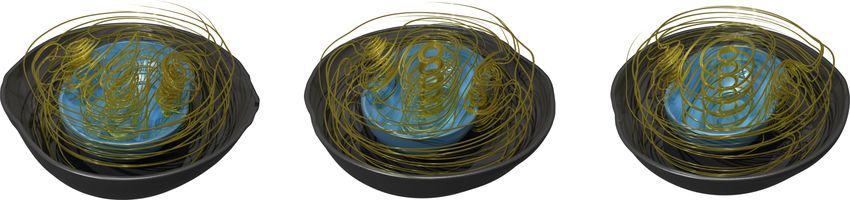
2

   For the simpler case of isolated uniformly rotating NS, the      nal or strict upper limits. In order to support the development
stability conditions are well understood. There is a maxi-          of postmerger-GW data analysis methods, we make the wave-
mum mass that depends only on the EOS. In the supramas-             forms extracted from our simulations publicly available [26]
sive range, i.e. between the maximum masses of nonrotating          as a qualitative example.
and uniformly rotating NS, a minimum angular momentum is
required. On timescales .0.1s however, one has to take into
account that the remnant is not uniformly rotating and that a                               II.   METHODS
significant fraction of total mass and angular momentum can
be located in the disk outside the NS remnant.                                               A.   Evolution
   For the important case of hypermassive NS remnants, dif-
ferential rotation is needed to prevent collapse. It is a popular      The general relativistic hydrodynamic equations are
assumption that collapse is caused by the dissipation of the        evolved numerically using the code described in [27, 28]. The
differential rotation. Should this be the only important as-        code utilizes a finite-volume high resolution shock capturing
pect, then the collapse delay depends on the effective viscos-      scheme in conjunction with the HLLE approximate Riemann
ity, which is not well constrained as it may depend on small        solver and the piecewise parabolic method for reconstruct-
scale magnetic field amplification. However, numerical simu-        ing values at the cell interfaces. We neither include magnetic
lations prove that merger remnants emit strong GWs. Since           fields nor neutrino radiation, and the electron fraction is pas-
short-lived remnants are close to collapse already, collapse        sively advected along with the fluid. Our numerical evolution
could be triggered by a relatively small angular momentum           employs a standard artificial atmosphere scheme, with zero
loss. It might well be the case that the collapse delay is mainly   velocity, lowest available temperature, and a spatially constant
determined by such losses instead of viscosity, or that both as-    density cut of 6 × 10⁵ g/cm3 .
pects are relevant.                                                    The matter equation of state is computed using a three-
   The overall rotation profile of merger remnants, which is a      dimensional interpolation table, where the independent vari-
key aspect for stability, has been studied in many numerical        ables are density, temperature, and electron fraction. For the
simulations [10–12, 19–23]. All these studies find a relatively     simulations in this work, we employ the SFHO EOS [29],
slow rotation of the core, and a maximum rotation rate in the       which incorporates thermal and composition effects. The EOS
outer parts of the remnant. The typical mass distribution in        was taken from the CompOSE EOS collection [30]. The ta-
the remnant core seems in fact to be similar to that of a nonro-    ble only contains temperatures above 0.1 MeV. In the context
tating NS [10, 11, 19, 21]. This led to the conjecture that the     of a binary NS (BNS) merger simulation, this is not problem-
collapse occurs once the remnant core density profile matches       atic since the thermal pressure at this temperature is negligible
the one in the core of the maximum-mass nonrotating NS [19].        to the degeneracy pressure except for very low densities. Al-
This conjecture was validated for a small number of examples        though dynamically ejected matter becomes diluted, it is also
[19, 21] but remains unproven in general.                           very hot and therefore not affected.
   The works above also revealed that the fluid flow can be            The spacetime is evolved using the McLachlan code [31],
more complex than just axisymmetric differential rotation,          which is part of the Einstein Toolkit [32]. This code imple-
featuring secondary vortices (see [11, 19, 20]). However,           ments two formulations of the evolution equation: the BSSN
those results are restricted to the equatorial plane, and little    formulation [33–35], and the newer conformal and spatially
is know about the 3D structure. The analysis of fluid flow pat-     covariant Z4 evolution scheme described in [28, 36]. Here we
terns in numerical simulations is complicated because early         use the latter because of its constraint damping capabilities.
merger phase is not fully stationary. Remnants show strong          We employ standard gauge conditions, choosing the lapse ac-
oscillations and can undergo a drift of compactness and rota-       cording to the 1 + log-slicing condition [37] and the shift vec-
tion rate within few dynamical timescales. A further difficulty     tor according to the hyperbolic Γ-driver condition [38]. At
arises from the coordinate choices in numerical simulations,        the outer boundary, we use the Sommerfeld radiation bound-
which are not well suited for studying the remnant shape [10].      ary condition.
   In this work, we focus on studying the three-dimensional            The time integration of the coupled hydrodynamic and
structure of merger remnants obtained when including only           spacetime evolution equations is carried out using the Method
the most basic ingredient of general relativistic hydrodynam-       of Lines (MoL) with a 4th-order Runge-Kutta scheme. Fur-
ics, while neglecting magnetic fields, effective magnetic vis-      ther, we use Berger-Oliger moving-box mesh refinement pro-
cosity, and neutrino radiation transport. We will analyze the       vided by the Carpet code [39]. For tests of the code, we
outcome of two simulations compatible with GW170817 in              refer the reader to [27, 28].
depth. For this, we develop novel postprocessing and visu-             In total, we use six refinement levels, each of which has
alization methods. We also investigate the evolution of the         twice the resolution of the next finer one. The four coars-
angular momentum distribution, using different measures.            est levels consist of a simple hierarchy of nested cubes cen-
   For GW170817, all useful information about the post-             tered around the origin. The two finest levels consist of nested
merger phase comes from the optical counterparts. No GW             cubes that follow each of the stars during inspiral. Near
signal could be detected after merger [24, 25]. Future obser-       merger, those are replaced by non-moving nested cubes cen-
vations of similar events with third-generation GW antennas         tered around the origin. The finest grid spacing is 221 m. The
might also include direct detection of a postmerger GW sig-         outer boundary is located at 950 km, and the finest level after
3

merger covers a radius of 28 km. Finally, we use reflection
                                                                    TABLE I. Initial data parameters: MB denotes the total baryonic
symmetry across the orbital plane.
                                                                    mass of the binary, Mc the chirp mass, M1 and M2 the gravitational
                                                                    masses of the stars, q = M2 /M1 the mass ratio, Λ1 and Λ2 the
                                                                    dimensionless tidal deformability of the stars, and Λ̃ the effective
                        B.   Initial data                           tidal deformability.
                                                                    Model                             Q10                         Q09
   In this work, we evolve binaries with a chirp mass of            MB [M     ]                      3.001                       3.008
Mc = 1.187 M , which is compatible with the very pre-               Mc [M    ]                       1.187                       1.187
cise measurement result of Mc = 1.186+0.001 −0.001 M for GW         M1 [M    ]                       1.364                       1.438
event GW170817 [2]. We consider the equal-mass case and             M2 [M    ]                       1.364                       1.294
one unequal-mass system with mass ratio q = 0.9. The NSs            q                                 1.0                         0.9
in our models are non-spinning, i.e. we use irrotational initial    Λ1                                396                         280
data. However, note that spin can have an impact on many as-        Λ2                                396                         551
pects discussed here, as demonstrated, e.g., in [20, 40–42] for     Λ̃                                396                         396
different systems. The characteristic properties of our models
are listed in Table I.
   As initial data EOS, we use the lowest temperature of            find that the maximum baryonic mass for a uniformly rotating
0.1 MeV that is available in the SFHO EOS. The initial              NS is 2.86 M . Based on comparisons in [11, 51], we do not
electron fraction for a given density is set according to β-        expect thermal contributions in the heated merger remnant to
equilibrium. This approximation to the zero-temperature EOS         significantly increase this maximum. The total baryonic mass
breaks down at very low densities because the thermal pres-         of our BNS models is well above the maximum allowed for
sure contribution becomes important and stays constant once         uniformly rotating models. Even allowing for atypically large
it is dominated by the photon gas. To avoid technical prob-         mass ejection of 0.1 M , the remnant is therefore hypermas-
lems determining the NS surface, we therefore replace the fi-       sive, i.e., it requires non-uniform rotation to delay collapse.
nite temperature table at densities below 1.4 × 10⁷ g/cm3 by        We therefore expect BH formation within tens of ms after
a matching polytropic EOS (with adiabatic exponent 1.58).           merger.
   The effective tidal deformability Λ̃, which encodes the im-
pact of tidal effects on the gravitational waveform during co-
alescence, is almost identical for the two mass ratios (in con-
trast to the individual deformabilities). The value of Λ̃ is com-                       C.   Coordinate Systems
patible with upper limits inferred for GW170817 under the as-
sumption of small NS spins [1, 2, 43, 44]. The statistical inter-      The standard 1+log and gamma-driver gauge conditions
pretation of the lower confidence bounds given in [2, 43, 44] is    used during evolution are well suited to prevent catastrophic
called into question [45], but in any case Λ̃ is well above those   gauge pathologies, but they are not designed to recover ax-
limits for our models. We also note that the Bayesian model         isymmetric coordinates when the spacetime approaches a
selection study [18] does not rule out even the zero tidal de-      mostly axisymmetric stationary phase. The coordinate sys-
formability case.                                                   tem present after merger depends not on the final mass distri-
   We note that our model is not compatible with the lower          bution, but on the whole history of the evolution. Therefore,
limit Λ̃ > 450 derived in [46] using inferred ejecta mass re-       one cannot rely on the coordinate-dependent quantities, e.g.
quirements for kilonova observation AT2017gfo. However,             multipole moments expressed in coordinates, to measure any
this value is based on an invalid assumption about the relation     deviations from axisymmetry.
between disk mass and effective tidal deformability. A first           In [10], we developed a postprocessing procedure to obtain
counterexample was found in [21] and a systematic investiga-        a well defined coordinate system in the equatorial plane with
tion [47] provided more. Revised fitting formulas presented in      the following properties 1. The radial coordinate is the proper
[48] exhibit large residuals and the search for robust analytic     distance to the origin along radial coordinate lines 2. The an-
modeling of ejecta masses is an ongoing effort. In any case,        gular coordinate is based on proper distance along arcs of
the disk and ejecta mass is computed in our simulations and         constant radial coordinate 3. On average, the radial coordi-
will be compared to values inferred from the kilonova directly.     nate lines are orthogonal on the angular ones, thus minimiz-
   In order to compute BNS systems in quasi-circular orbit,         ing twisting. If the spacetime is indeed axisymmetric (with
we employ the LORENE code [49]. Since we are mainly in-             axis orthogonal to the equatorial plane of the simulation coor-
terested in the qualitative post-merger behavior, we take no        dinates) then so are the new coordinates.
steps to reduce the residual eccentricity inherent in the quasi-       In this work, we also want to study the 3D structure of the
stationary approximation, and we chose an initial separation        remnant. We therefore need to extend the coordinate system
that corresponds to no more than 6 full orbital cycles before       above from the equatorial plane. However, the metric was not
merger.                                                             saved in 3D in our simulations, which precludes a generaliza-
   Using the same EOS as for the initial data, we computed the      tion in the same spirit. Instead, we use an ad-hoc construction
baryonic mass for sequences of NSs rotating uniformly with          as follows. First, we apply the same coordinate transforma-
rate at the mass shedding limit (using the RNS code [50]). We       tion as within the equatorial plane to all planes with constant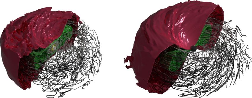
4
z-coordinate. Using the metric saved along the z-axis during where W is the Lorentz factor of the fluid with respect to Eu-
the simulation, we transform the z-coordinate as z → z 0 (z) lerian observers, dV is the proper 3-volume element and γ is
such that on the z-axis, the new z-coordinate is the proper the determinant of the 3-metric. On the numerical level, the
distance to the equatorial plane along the axis. Away from baryonic mass definition is complicated by the use of an artifi-
the axis, the new z-coordinate is only an approximation to the cial atmosphere. Our numerical volume integrals of baryonic
proper distance to the equatorial plane. mass exclude any grid cell set to atmosphere.
The resulting 3D coordinate system allows to judge ax- To obtain the mass of dynamically ejected matter, we com-
isymmetry in the equatorial plane, and it allows to assess pute the time-integrated flux of unbound matter through sev-
oblateness since distances along the z-axis and within the eral coordinate spheres with radii between 73–916 km. For
equatorial plane are exact proper distances. In the meridional each sphere, we then add the volume integral of residual un-
planes a coordinate circle might still show some deviations bound matter still present within the same sphere at the end
from a proper sphere, except on z-axis and the equator. In of the simulation. Matter is considered unbound according
the rest of this work, we refer to this coordinate system as to the geodesic criterion ut < −1, where u is the 4-velocity,
postprocessing coordinates to distinguish from simulation co- and the artificial atmosphere is excluded. This criterion as-
ordinates. sumes force-free ejecta and therefore becomes more accurate
From previous experience [11, 19, 20], we expect that the at larger radii.
remnant is changing only slowly when viewed in a coordinate The combined measure for the ejecta mass alleviates draw-
system rotating with a certain angular velocity, which is also backs of using flux or volume integrals only. When using only
changing slowly (also compare the animations provided in the the flux through an extraction sphere, one is either restricted
supplemental material of [20]). In other words, we expect an to small extraction radii to ensure that all ejecta are accounted
approximate helical Killing vector. for, or forced to evolve the system long enough to allow all
To extract the rotating pattern of mass distribution and ve- ejecta to reach the extraction radius. When using only vol-
locity field, we construct corotating coordinates as follows. ume integrals, they have to be computed before significant
First, we perform a Fourier decomposition with respect to φ amounts of ejecta leave the computational domain. Such in-
(in postprocessing coordinates) in the equatorial plane. We tegrals then include matter at small radii where the geodesic
then compute a density-weighted average to get the phase of criterion is unreliable, and miss ejecta that become unbound
the dominant m = 2 density deformation as function of time. later. The combined measure allows meaningful comparison
We further apply a smoothing by convolution with a 2 ms long over a larger range of extraction radii. For the cases at hand,
Hanning window function to suppress high frequency contri- we find negligible differences for radii & 400 km, and use the
butions. We then apply the opposite rotation to the 3D post- outermost radius 916 km for quoting ejecta masses.
processing coordinates at each time to obtain postprocessing We employ a similar approach for estimating the escape
coordinates corotating with the main deformation pattern. velocity. In a stationary spacetime, the velocity that a fluid
element would reach after escaping the system on a geodesic
trajectory is v∞2
= 1−u−2
t . Again, we consider both the ejecta
leaving the system through a spherical extraction surface dur-
D. Diagnostic Measures ing the simulation, and the unbound matter still within the
domain at the end. Both contributions are filled into a mass-
In order to extract gravitational waves, we decompose the weighted histogram of the escape velocity. This way, we ac-
Weyl-scalar Ψ4 into spin-weighted spherical harmonics, con- count for the fastest components via the flux as well as the
sidering all multipole coefficients up to l = 4. The strain is slowest ones via the unbound matter at final time.
computed by time integrating using the fixed-frequency inte- For technical reasons, we first combine all ejecta at a given
gration [52] method with a low-frequency cutoff at 500 Hz. time within thin spherical shells Vs with radius Rs and thick-
The fluxes of energy and angular momentum are also com- ness δRs . For those, we compute the volume integrals
puted using multipole components up to l = 4. We use a fixed Z Z
1
extraction radius Rex = 916 km, close to the outer boundary Ws = ut W ρu dV, Ms = W ρu dV (2)
of the computational domain. We do not extrapolate the signal Ms V s Vs
to infinity as we expect the finite resolution error to dominate
where ρu is the density of unbound matter in the fluid rest
the error due to finite extraction radius.
frame. From the above measures, we attribute an average
To describe the distribution of matter, we use the bary- escape velocity vs2 = 1 − Ws−2 to each shell. To compute
onic mass density ρ, defined as baryon number density in the the above integrals at each time for each radius, we employ a
fluid rest frame times an arbitrary mass constant (in this work simple and robust technical implementation based on creating
1.66 × 10⁻²⁷ kg). Baryon number conservation implies a histograms of all numerical grid cells, binned by radius, and
conserved current uµ ρ, with u being the fluid 4-velocity. The weighted by the integrands.
total baryonic mass within a volume can only change by mat- Another quantity relevant for our study is the ADM mass
ter leaving the boundary, and is given by of the system. This measure is formally defined for the whole
spacetime, as there is no locally conserved energy in GR. It
√
Z
MB = W ρ dV, dV = γ d3 x (1) can be expressed either via surface integrals at infinity, or 3-
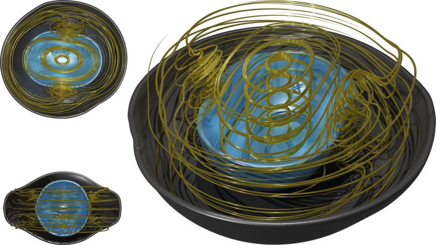
V volume integrals over a spacelike hypersurface of a given fo-5 liation of spacetime. When restricting either formulation to lative summation over the bins. Using this method, we inte- sufficiently large but finite region, such that the outer bound- grate the (i) proper volume (ii) baryonic mass (iii) ADM mass ary lies in the weak field regime, then the ADM mass is not (iv) ADM angular momentum (v) Komar angular momentum constant but changes by the amount of energy carried away by approximation (vi) estimated mass of unbound matter. GW. We thus compute a time-dependent ADM mass from the We note that the 3-dimensional isodensity surfaces in 4- ADM mass of the initial data minus the integrated GW energy dimensional spacetime are gauge-independent. The corre- flux. sponding volume integrals within a time slice depend only on As a heuristic measure of energy distribution, we monitor the time slicing but not on the spatial gauge. In contrast, in- the integrand of the ADM mass volume integral as well. How- tegrals over spheres of constant coordinate radius depend on ever, we stress that this is not gauge invariant as it depends on the spatial coordinates. In order to reduce this dependency, the chosen foliation of spacetime. Our motivation is to split we parametrize the spheres by the enclosed proper volume. the total ADM energy into contributions of the remnant NS The only remaining gauge ambiguity (beside the time slicing) and the surrounding disk. is given by the shapes of the coordinate spheres, but not their We also need to consider the gravitational radiation still in- overall extent. side the computational domain. As a practical measure, we Similarly, we also parametrize the integrals within isoden- use the following: considering the region between R0 < r < sity surfaces by the enclosed proper volume. Within the rem- Rex , we define a GW energy at time t as the integrated GW nant NS, where the mass distribution is roughly spherical, flux through Rex over the time interval (t, t + Rex − R0 ). We the two methods of defining radial mass distribution should compute this measure for R0 as low as 100 km (around the roughly agree. This is not the case for the torus-shaped disk. wavelength of a 3 kHz signal). In other words, we associate For convenience, we will sometimes express proper volumes an energy loss of the remnant at a given time with the GW in terms of the radius of Euclidean spheres with same volume luminosity at a large extraction radius at the time when the ra- (“volumetric radius”, RV ). diation from radius R0 has reached the extraction radius. This Based on the above integrals, we can define a measure for can only provide a qualitative picture, as the measure is build the compactness of any volume as the baryonic mass divided on concepts valid in the weak field limit / wave zone. by the volumetric radius. The compactness of isodensity sur- For the angular momentum, we use the volume integral for- faces as function of volumetric radius a has a maximum. We mulation of the ADM angular momentum, similarly to the refer to the region within this maximum-compactness surface ADM mass above. As for the mass, we compute the GW an- as the “bulk”. We use the bulk definition to divide the mat- gular momentum loss, at the same extraction radius. For ax- ter distribution after merger into a remnant and a disk, but we isymmetric spacetimes, another angular momentum definition stress that this is somewhat arbitrary as there is a smooth tran- is given by Komar. Since the system approaches a roughly sition. axisymmetric state after merger, it makes sense to use the Ko- mar angular momentum. We note that the Komar measure is more closely related to the fluid in the sense that there are no III. RESULTS contributions of vacuum, horizons aside, and, consequently, no contributions of GW radiation present in the system. For A. Overall dynamics exact definitions of ADM and Komar quantities, we refer to [53]. In the following, we provide a broad overview on the The post-merger evolution is not exactly axisymmetric, the merger outcome. Key quantities are summarized in Table II. postprocessing coordinates are not available during the simu- Qualitatively, both cases are very similar. For the example of lation, and we avoid storing all metric quantities as 3D data. the q = 0.9 case, we visualize the evolution timeline in Fig. 1. Therefore, we use an approximation to the Komar angular mo- The coalescing NS merge into a hypermassive NS (HMNS) mentum that is obtained by integrating the φ-component (in which collapses to a BH after a delay on the order of ≈10 ms. simulation coordinates) of Sφ , the evolved quasi-conserved The HMNS is embedded in a massive debris disk created dur- momentum density. This is trivial to compute during the sim- ing merger. The disk is strongly perturbed by interactions with ulation, but becomes exact only if the φ-coordinate is a Killing the remnant, and settles to a more stationary state shortly after vector field. the BH is formed. Besides volume integrals over the full domain, we are in- Quantitatively, we observe some differences between the terested in the radial distribution of the integrands. For this, two mass ratios. Most notably, the collapse delay is about we employ a numerical method developed in a previous study 0.25% shorter for the unequal mass case. This can be seen in [11]. This method allows an efficient computation of vol- Fig. 2 showing the evolution of the remnant density. We stress ume integrals (i) within spheres of constant coordinate radii that in general, the delay time for a given mass is very sensi- as function of radius, and (ii) within regions above given mass tive to numerical errors, because the system is at the verge of densities ρ as function of ρ. It works by adding the inte- collapse (we will discuss the evolution leading to collapse in grand (including the volume element) in each numerical cell later sections). However, since both simulations employ the into onedimensional histograms binned in terms of coordi- same resolution, grid setup, and numerial method, we expect nate radius and density, respectively. The volume integrals the difference of the delays to be more robust than the absolute can then be obtained during post-processing simply by cumu- values.
6

                                                                                                                                     q=1
                                                                                    1016

                                                                          [g/cm3]
                                                                                    1015

                                                                                                     max                             q = 0.9
                                                                                                     blk
                                                                                    1016

                                                                          [g/cm3]
                                                                                    1015
FIG. 1. Overview of the evolution phases for the q = 0.9 case. Time
runs from lower right to upper left, while the other two dimensions                        14         12        10          8          6       4     2   0
correspond to the orbital plane. The transparent green surface corre-                                                           t tah [ms]
sponds to a fixed density of 5 × 10¹³ g/cm3 , highlighting the evolu-
tion of the merged NS and the coalescing NS shortly before merger.
The solid red surface corresponds to a density of 1011 g/cm3 , as a     FIG. 2. Post-merger evolution of mass density in the remnant for the
proxy for the denser parts of the disk. To avoid occlusion, one half-   equal mass case (top panel) and unequal mass case (bottom panel).
plane was cut away. The blue surface marks the apparent horizon         The solid curve shows the maximum baryonic mass density in the
extracted during the simulation. To give an impression of the thermal   fluid frame. The dotted curve shows an average density given by
evolution inside the remnant, we rendered hot, dense regions as light   bulk mass per bulk volume (see text). The time refers to coordinate
emitters (without absorption). The time coordinate was compressed       time. For comparison, the horizontal lines show the central density
by a factor 0.05 with respect to the spatial coordinates in geometric   (dashed) and average bulk density (dash-dotted) of the maximum-
units, such that light cones would appear almost orthogonal to the      mass TOV solution. The vertical lines mark the time of merger and
world tube of the remnant.                                              formation of an apparent horizon.

                                                                                                 99%            BH loss             Max TOV                  15
   For a remnant close to collapse, one can expect that small                        40          98%            Max Unif.           Core
                                                                                                                                                             14
changes of the initial parameters, mainly the total mass,
should lead to large changes of the delay. This is however                           20                                                                      13

                                                                                                                                                                       )
                                                                                                                                                                 log10 [g/cm3]
not a drawback. Any observational constraint on the delay
                                                                                                                                                             12
                                                                          z[km]

translates into a stronger constraint on the total mass. In this                      0

                                                                                                                                                                       (
context, the relevant numerical uncertainty is not the (large)                                                                                               11
error of the delay for a given mass, but the (smaller) error in                      20
                                                                                                                                                             10
the total mass that leads to a given collapse delay.
   We emphasize that our non-magnetized simulations ex-                              40                                                                      9
clude the possibility of effective magnetic viscosity due to
                                                                                                60         40        20       0       20       40   60
small-scale magnetic field amplification. Such effects might                                                                x[km]
reduce the collapse delay further. Since it is difficult to pre-
dict the impact of mass ratio on magnetic field amplification,
we also cannot exclude an impact on the relation between col-           FIG. 3. Mass distribution in the meridional plane 2 ms before ap-
                                                                        parent horizon formation, averaged over a time window ±1 ms. The
lapse delays and mass ratio. For further discussion, see [54]
                                                                        color scale shows the baryonic mass density. The contours mark
and the references therein.                                             densities for which the corresponding isodensity surfaces contain se-
   The HMNS is smoothly embedded within a debris disk.                  lected mass fractions. We show the contours for 99%, 98%, the mass
The structure of the disk is shown in Fig. 3 for the example            swallowed by the BH within 1 ms after formation, the maximum
of the q = 0.9 case. The innermost part of the disk falls               mass of uniformly rotating and nonrotating NS, and the (nearly iden-
into the BH after the remnant collapses. After collapse, the            tical) mass of the nonrotating NS best approximating the core (see
remaining disk mass is around 0.05 M (see Table II). The                text).
disk contains enough matter to supply a wind that could ex-
plain the red component of the kilonova AT2017gfo observed
after GW170817, with an inferred mass ≈0.04 M [7]. It                   remnant into the disk. This was already observed for different
would, however, require an effective mechanism in order to              models in previous studies [11, 21]. Since the remnant life-
expel around 80% of the disk. The structure of the disk after           time also increases with decreasing mass, the final disk mass
BH formation is shown in Fig. 4 for the q = 0.9 example.                should depend even more strongly on the total mass. Con-
   As a general trend, we expect that for fixed EOS and mass            versely, we expect a more massive disk for a system with the
ratio, systems with lower total mass possess a more massive             same total mass, but obeying a different EOS for which the
disk after merger (compare, for example, [46]). We will fur-            maximum NS mass is slightly larger.
ther show that in our cases, some matter is migrating from the             We observe significant dynamical mass ejection during
7
13
AH 1.5% 0.8% 0.5% q=1 24.0
40
12 15
23.7
(t tmerger) [ms]
20
10 23.4
)
11
log10 [g/cm3]
z[km]
0 23.1
ub [g/cm])
10 5
(
22.8
20
0 22.5
log10(4 r2
9
15.0 q = 0.9
40 22.2
8 12.5
(t tmerger) [ms]
60 40 20 0 20 40 60 10.0 21.9
x[km] 7.5
21.6
5.0
2.5 21.3
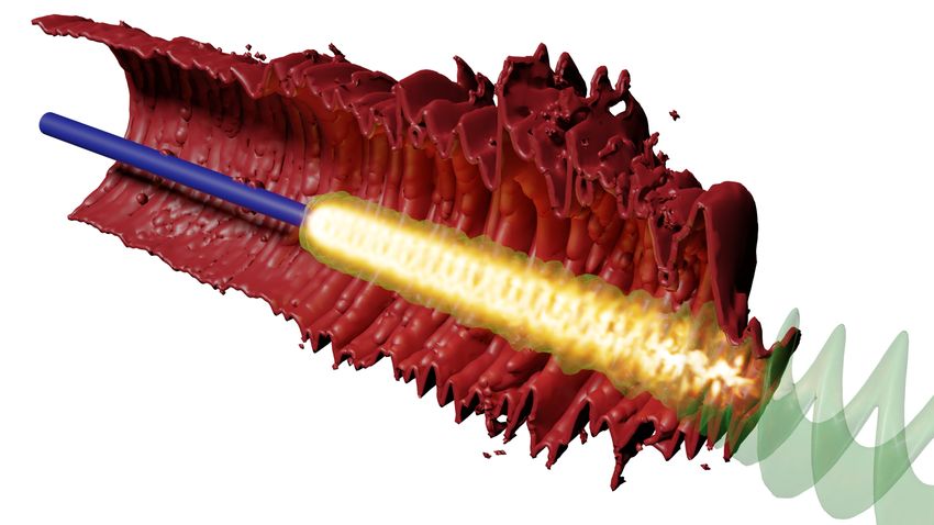
FIG. 4. Like Fig. 3, but showing the time 2 ms after apparent horizon
0.0
formation. The density contours contain selected fractions of initial 0 200 400 600 800
total baryonic mass (excluding the BH interior). r [km]
FIG. 5. Radial distribution of unbound matter versus time after
TABLE II. Key parameters of merger outcome. MBH and JBH are merger. The color scale corresponds to unbound mass per radial dis-
black hole mass and angular momentum 5.0 ms after formation. tance, where matter is considered unbound according to the geodesic
FBH is the GW frequency from quasi-normal-mode ringdown for criterion. The horizontal lines mark the time of BH formation.
the given mass and spin. Mblk and Rblk are bulk mass and bulk
volumetric radius, extracted 1.0 ms before collapse. Rows νcnt and
νmax denote the remnants central and maximum rotation rates com-
similar numerical setup found a finite resolution error of the
puted 1.0 ms before collapse. fmerge is the gravitational wave in-
stantaneous frequency at the time of merger, fpm is the frequency dynamical ejecta mass around 20%. In our case, an additional
of the maximum in the post-merger part of the gravitational wave — and likely dominant — source of uncertainty is the depen-
power spectrum. Row Mdisk provides the baryonic mass outside dence of dynamical ejecta mass on the lifetime of the remnant.
the apparent horizon, excluding unbound matter, at time 6.0 ms af- The latter can be extremely sensitive to errors if the remnant is
ter collapse. Mej is the estimate for the total mass of dynamically on the verge of collapse. It is therefore difficult to estimate the
ejected matter, v∞ refers to the median, 5th and 95th percentiles of error without expensive tests with much higher resolutions,
the mass-weighted escape-velocity distribution of ejected matter. but we suspect that the error could easily reach a factor two.
Model Q10 Q09 Comparing to other results in the literature, we find a disk
MBH [M ] 2.55 2.57 mass that is an outlier to the phenomenological fit of disk
JBH /MBH2
0.66 0.67 mass in terms of effective tidal deformability that was pro-
FBH [kHz] 6.56 6.52 posed in [46]. Other counterexamples were already found
Mblk [M ] 2.56 2.59 in [21, 47]. We also note that [55] performed a simulation
Mblk /Rblk 0.31 0.31 that corresponds almost exactly to our q = 1 setup, except
νcnt [kHz] 0.96 0.87 that it includes neutrino radiation. They quote a lower ejecta
νmax [kHz] 1.76 1.71 mass (2.8 ± 0.7) × 10−3 M as well as a lower disk mass
fmerge [kHz] 1.94 1.94 (1.9 ± 0.7) × 10−2 M , but also find a remnant lifetime that
fpm [kHz] 3.38 3.35
is around 3 times shorter than for our simulations.
Mdisk [10−2 M ] 5.5 4.6
Mej [10−2 M ] 1.7 0.8
Our results depicted in Fig. 5 show that mass is continu-
v∞ [c] 0.16+0.08 0.14+0.09 ously ejected during the HMNS lifetime. The differences in
−0.11 −0.08
lifetime could thus account for the tension regarding the ejecta
masses. Similarly, it might account as least partially for the
lower disk mass. The difference in lifetime could be due to
merger and during the remnant lifetime. As shown in Fig. 5, finite resolution errors alone, but it is also possible that the in-
several independent mass ejections are launched, mostly from clusion of neutrino transport has an influence on HMNS close
radii .100 km. The individual ejected components merge, to collapse. In any case, the result that increasing the lifetime
because of their velocity dispersion, and leave the system as a of a HMNS can lead to larger disk and ejecta masses suggests
single ejecta component. It seems that the pressure waves in- that fitting these quantities in terms of the binary parameters
jected into the disk (see also Fig. 1) by the HMNS also result as in [46, 48] is challenging for the parameter ranges resulting
in matter ejection from the disk. in short-lived HMNS. We propose to include the lifetime as
The ejecta mass as extracted from the numerical results is an unknown in the fit, not just because of the sensitivity with
given in Table II. We stress that in general, ejecta masses ex- regard to total mass and numerical errors, but also because the
tracted from numerical simulations are affected comparably lifetime may be affected by physical effects such as magnetic
strong by the numerical errors. Convergence tests presented viscosity that are essentially unknown.
in [19] for simulations of a long-lived remnant using a very The spectral evolution of the kilonova depends strongly on8
the ejecta velocity. Table II reports the median of the veloc- with next-generation instruments. Apart from the modula-
ity distribution extracted from our simulations as described in tion, the frequency also shows a slow drift towards higher
Sec. II D, together with 5th and 95th percentiles. The values frequencies. This correlates with a change in remnant com-
refer to the outermost extraction radius, but we also compared pactness that will be investigated in Sec. III C. Once the BH
smaller ones. We find that the median and 5th percentile are is formed, the signal amplitude decays quickly while the fre-
stable outside 400 km, whereas the 95th percentile continu- quency reaches the value that is expected for a BH with the
ously decreases and should be considered as unreliable. Given mass and spin found in our simulations (this can only be ob-
that the fastest components are those running into the artificial served briefly as the amplitude quickly becomes too small for
atmosphere, the deceleration is likely unphysical. Another numerical study).
source of uncertainty is that an earlier collapse of the HMNS The other two curves shown in Fig. 6 are predictions from
would result in less ejected mass, but faster median velocity, waveform models commonly used in the LIGO and Virgo data
because ejecta launched at later times tend to be slower for the analysis. In order to visually compare them to the numeri-
cases at hand. cal simulations and hybridize the waveforms, we aligned each
The mass and velocity found in our numerical results are model with the respective signal from our numerical simu-
both about a factor two lower than the estimates inferred by [7] lation using the following procedure. First, after generating
for the blue component of the kilonova AT2017gfo. However, the model waveforms using the same masses as our numer-
because of the uncertainties discussed above, we cannot make ical simulations and zero spins, we align the signals in time
a conclusive statement if the dynamical ejecta mass for the by minimizing the L2 norm of the difference between the
SFHO EOS is compatible with the observed kilonova. phase velocities ω = 2πF , taken over the time interval where
Besides mass and velocity, kilonova models such as [7] ω ∈ [3850, 6000] rad/s. Second, we adjust the phase offset in
also predict a strong dependency on the composition of the the model such that the average phase difference between the
ejecta. The initial electron fraction of the neutron-rich ejecta numerical data and the models vanishes in the interval speci-
is strongly affected by neutrino radiation (see, e.g., [56]). fied above. The only free choice in this procedure is the inter-
Since those are not included in our study, we refrain from dis- val used for the alignment. It has to be chosen small enough
cussing the ejecta composition, but note that once again the to align the waveforms in the “early” inspiral of the numerical
lifetime of the HMNS has a direct impact on an observable. simulation. On the other hand, the size of the interval has to be
It should also be noted that disk evolution and ejecta might large enough so that the frequency evolves significantly [60].
be sensitive to magnetic field effects, which are not included Otherwise the time shift would only be weakly constrained.
here. For the example of a system with large initial magnetic The range defined above is an empirically found compromise
field that was studied in [12], the entire disk was driven to that is shown as a shaded band in Fig. 6.
migrate outwards (but not necessarily ejected). On the other One model used for comparison is the binary BH (BBH)
hand, a reduction of remnant lifetime by magnetic viscosity model IMRPhenomD [58, 59] that does not incorporate tidal,
might result in less dynamical ejecta and a less massive disk. finite-size effects of NSs. We would therefore not expect it
to accurately describe the late inspiral and merger of a BNS.
However, the tidal effects for the cases at hand are small in
B. Gravitational Waves the frequency range used for the fitting, quite likely within the
numerical error of the simulations. We stress that the aim of
In this section, we present the GW signals extracted from our study is not the accurate modeling of the inspiral phase,
the simulations as described in Sec. II D. We compare the which would require very high resolution (see, e.g., [61]).
dominant spherical harmonic ` = |m| = 2 mode with pre- Just before merger, the BH model and NS simulation start
dictions from theoretical waveform models, produce a hybrid to diverge significantly. A BBH with the same masses, fol-
waveform combining analytical inspiral data with the result lowing the alignment of the model and simulations used here,
from our numerical simulations, and quantify the initial ec- would perform about 1.5 orbits more than the BNS before
centricity of our simulations through the GW frequency. merging. The most striking difference then, of course, is
Figure 6 shows the plus polarization of the GW from three that the BBH forms a remnant BH immediately at merger,
data sets. The purple line is the result extracted from the nu- whereas our BNS mergers result a short-lived HMNS which
merical simulation. Three characteristic phases are clearly emits strong GW until it collapses to a BH. During merger, the
identifiable. During the inspiral, the amplitude and frequency signal shows an amplitude minimum accompanied by a phase
gradually increase until the maximal amplitude of the com- jump that is characteristic to BNS mergers [20], but we ob-
plex strain, h = h+ − i h× , is reached at t = tmerger . The serve none of the secondary minima/phase jumps which can
following post-merger oscillation is characterized by an over- sometimes be present. We will revisit this point in Sec. III D.
all slowly decaying amplitude. Figure 7 shows the instan- The mass of the final BH that would result from the analo-
taneous frequency, F = (2π)−1 dφ/dt, where φ is the GW gous BBH case can be computed using the fit to nonprecess-
phase extracted as the argument of the complex strain h. It ing NR simulations by Varma et al [62]. The fit predicts that
exhibits a characteristic modulation, with an initially large but BBH mergers in the mass ratio 0.9 and 1 case produce rem-
rapidly damped amplitude. As we will show in Sec. III C, nants with mass 2.60 M and dimensionless spins of 0.68 and
this modulation is an imprint of the remnant’s radial oscil- 0.69, respectively. Somewhat surprisingly, this agrees within
lations. Such an imprint might be exploited in observations a few percent with the parameters of the BH formed in the9
1e 22
PhenD PhenDNRTv2 NR q = 0.9
5
0
h+
5
1e 22
q=1
5
0
h+
5
30 20 10 0 10 2 1 0 1 2
t tmerger [ms] t tmerger [ms]
FIG. 6. The GW signals extracted from our simulations (blue) as observed face-on at a distance of 40.7 Mpc. We extend the inspiral with the
BNS model IMRPhenomD NRTidalv2 [57] (orange), aligned with the numerical data over the grey shaded region. For comparison, we also
include the BBH model IMRPhenomD [58, 59] (gray dashed lines).
BNS case, shown in Table II. The hybrid waveforms are released as data files [26] with
Waveform models that include tidal deformations of the this article to facilitate exploratory data analysis studies. How-
NSs and the resulting effect on the binary’s orbit are more ever, we caution that the accuracy of both the inspiral and
appropriate for the systems we simulate here. As an ex- NR data may not be sufficient for high-accuracy applications.
ample of current state-of-the-art models, we employ the Nevertheless, they may be used to estimate the order of mag-
IMRPhenomD NRTidalv2 model [57] that adds an NR- nitude at which differences in waveforms become measurable.
informed description of the tidal dephasing on top of the BH As an example, we calculate the mismatch between the hy-
model [63]. The model is also shown in Fig. 6. While visu- brids and the analytical waveforms shown in Fig. 6.
ally there is no difference to the BH model over the fitting re- The mismatch quantifies the disagreement between two sig-
gion, the effect of the tidal phase corrections becomes visible nals akin to an angle between vectors. We employ the standard
as a gradual dephasing in the earlier inspiral. The impression definition of the mismatch,
that the dephasing between BH and tidal model seems to in-
crease as one moves to earlier times is an artifact of aligning hh1 |h2 i
M(h1 , h2 ) = 1 − max , (5)
the models in the late inspiral. IMRPhenomD NRTidalv2 δφ,δt kh1 k kh2 k
does not attempt to model the merger and postmerger accu- Z f2
h̃1 (f ) h̃∗2 (f )
rately; it simply decays rapidly beyond the contact frequency hh1 |h2 i = 4 Re df, (6)
f1 Sn (f )
of the two NSs.
We use IMRPhenomD NRTidalv2 to construct hybrid
waveforms that cover the GW signal from the very early inspi- where h̃(f ) is the Fourier transform of h(t), ∗ denotes com-
ral starting at 20 Hz to the end of what was simulated numeri- plex conjugation, Sn (f ) is the power spectral density of the
cally. We smoothly blend the inspiral model and the NR data assumed instrument noise, and the mismatch is minimized
over the same region that we used for aligning the signals in over relative time (δt) and phase (δφ) shifts between the two
Fig. 6. The boundaries of this interval [t1 , t2 ] inform a Planck signals. khk2 = hh|hi is the norm induced by the inner prod-
taper function [64], uct. As examples, we calculate mismatches using the noise
curves provided in [65] for Advanced LIGO [66], LIGO Voy-
0,
t ≤ t1 ager [67] and the Einstein Telescope [68]. For simplicity, we
i−1
use the starting frequency of the hybrid, f1 = 20 Hz in our
h
2 −t1 2 −t1
T (t) = 1 + exp tt−t + tt−t , t1 < t < t2 ,
1 2 calculations. Note that the assumed instruments are sensitive
1, t ≥ t2
to lower frequencies, but as we mainly want to illustrate the
(3) effect of the merger and post-merger, our results are meaning-
ful even for this artificially chosen starting frequency.
which we use to construct a C ∞ transition with compact sup-
As we can see from the results in Table III, the hybrids dis-
port of the form
agree significantly more with the BBH model than with the
Xhyb (t) = T (t) XNR (t) + [1 − T (t)] Xinsp (t). (4) tidal NS model. MBBH is dominated by the tidal effects of
the inspiral, i.e., it reflects the difference between the tidal
Here, X(t) stands for the amplitude or phase of the complex inspiral model chosen for hybridization and the BBH model.
strain, which are hybridized individually. Note, however, that the mismatch is larger than it would be in10
able to measure the difference between our hybrid and the in-
TABLE III. Comparison of our hybrid waveforms with either the the
spiral tidal model out to a greater distance. We note that the
BBH model (IMRPhenomD) (first row) or the tidal inspiral model
(IMRPhenomD NRTidalv2) (remaining rows). We present mis- SNR contained in the hybrid waveform beyond the merger fre-
matches M assuming instrument noise curves for aLIGO second quency accounts for most of the mismatch we calculate, i.e.,
observing run O2, aLIGO design sensitivity, LIGO Voyager and the
khhyb (f > fmerger )k2
∼ 2M ∼ O 10−4 .
Einstein Telescope. The last two rows indicate at what SNR the hy- (9)
khhyb k 2
brid and the tidal inspiral model would distinguishable at the 90%
credible level (see text), and at which distance this SNR would be
achieved for optimally oriented binaries. While the mismatch and overall SNR may be affected by our
choice of lower cutoff frequency f1 , the distance we quote is
O2 aLIGO Voyager ET dominated by the post-merger and largely independent of the
Q09 Q10 Q09 Q10 Q09 Q10 Q09 Q10 specific choice of f1 . Hence, it defines the volume in which
MBBH [10−4 ] 51 52 120 110 49 49 96 98 the specific post-merger signal from our simulations is distin-
MBNS [10−4 ] 0.8 1.7 2.8 4.6 0.7 1.6 1.7 3.3 guishable from the tidal model without post-merger contribu-
SNR90 130 91 69 54 140 93 89 64
tion. A study of similar questions was published in [71]. We
D90 [Mpc] 13 19 48 62 100 160 380 530
stress that we do not address the more complicated question at
which distance the presence of an unknown post-merger sig-
nal can be observed.
a real parameter estimation study, where the masses and spins As a final application of our waveform comparison, we use
are not fixed, such that the BBH model could partly mimic the inspiral data to estimate the eccentricity of our NR sim-
tidal effects at the expense of biasing these parameters. On ulations. We do this by comparing the frequency evolution
the other hand, by comparing the hybrids with the same in- ω(t) = dφ/dt of the NR data with the quasi-circular data of
spiral waveform used for hybridization, we can quantify the the IMRPhenomD NRTidalv2 model. The residual differ-
effect of the merger and post-merger that is only present in ence
the hybrid. Those mismatches for all assumed instruments are ωNR − ωcirc
O(10−4 ). This might seem surprising at first, given that e.g., eω = (10)
the Einstein Telescope is more sensitive than aLIGO. How- 2ωcirc
ever, because the mismatch is based on the normalized inner can be fit by a sinusoidal oscillation added to a small linear
product, its value is determined by the relative weight between drift that absorbs any inaccuracies in the alignment. The am-
low and high frequencies as given by the noise spectral den- plitude of the oscillatory part of eω characterizes the eccen-
sity, and not by the instrument’s overall sensitivity. Choosing tricity of the NR simulation [72]. We find initial eccentricities
the same lower cutoff frequency f1 = 20 Hz for all instru- 0.010 and 0.009 for the equal-mass and mass ratio 0.9 simu-
ments exaggerates this effect. lation, respectively.
We can appropriately account for the actual detector sen-
sitivity by relating measurability of a difference between two
signals with the signal-to-noise ratio (SNR). Following the C. Radial Remnant Profiles
derivation in [69, 70], one finds that the difference between
the hybrid and the inspiral model is indistinguishable at the We begin our discussion of the remnant structure with the
p-probability level if average radial mass distribution shortly before the onset of
collapse. For this we use the measure introduced in Sec. II D.
khhyb − hBNS k2 < χ2k (p), (7) Fig. 8 shows the profile of baryonic mass contained within
isodensity surfaces versus the proper volume within the same
where χ2k (p) is a number derived from the χ2 -distribution surfaces. We also mark the bulk region defined in Sec. II D. As
with k degrees of freedom at which the cumulative proba- shown in Fig. 3, there is a smooth transition between remnant
bility is p. Here we consider the question at what SNR the core and surrounding disk. This is also reflected in the mass-
waveform differences are distinguishable at a 90% level for volume profile.
a one-dimensional distribution. Using the corresponding val- It is instructive to compare this profile to those obtained for
ues p = 0.9, k = 1 results in χ2k (p) = 2.71. Expanding the nonrotating NS with same EOS as the initial data. In a previ-
left-hand side of Eq. (7) for small M, we finally obtain ous work [11], we introduced a method to find a nonrotating
NS model (with same EOS as the initial data) for which the
min khhyb − hBNS k2 ≈ 2khhyb k2 M < χ2k (p), (8)
khBNS k profile of the core resembles the one of the remnant. To this
end, we compute the bulk mass versus bulk volume for the
which allows us to estimate the critical SNR (khhyb k) required whole sequence of nonrotating NS and find the intersection
to distinguish the two signals given their mismatch. The re- with the remnant mass-volume profile, provided that it does
sult is shown in the third row of Table III. Further assuming intersect.
an optimally oriented source overhead the detector, we can The sequence is shown in Fig. 8 and just barely intersects
calculate the luminosity distance at which the critical SNR the remnant profile, near the maximum mass NS model. The
is achieved. This last row in Table III follows the expected figure also shows the mass-volume profile of the correspond-
trend: more sensitive, future-generation instruments would be ing NS model, which we refer to as core-equivalent TOV11
8 3.0 q=1
7
2 × frot
max
q=1 Simulation
fGW Adv. LIGO 2.5
6 fmodel ET design
fBH Voyager 2.0
Mb [M ]
5 fradial 1.5
fvibrato
F [kHz]
4 1.0
3
0.5
2
0.0
1
0
3.0 q = 0.9
2.5
8
7
q = 0.9 2.0
Mb [M ]
6 1.5
Remnant
5 1.0 Bulk
0.5 TOV bulk
F [kHz]
4 Core equiv
3 0.0
0 2500 5000 7500 10000 12500 15000 17500 20000
2 V [km3]
1
0 FIG. 8. Total baryonic mass contained inside surfaces of constant
15 10 5 0 5 10 21.5 21.0 20.5
t tmerger [ms] log10(F h) density (blue curve) versus proper volume contained within the same
surfaces. The top panel shows the remnant for the equal mass case,
the bottom panel for the unequal mass system, both at a time 1 ms
FIG. 7. Left panels: time evolution of GW frequency fGW , maxi- before apparent horizon formation. The dot marks bulk mass and
mum rotation rate νmax , radial oscillation frequency fradial , and the bulk volume of the remnant (see text). For comparison, we show bulk
rate of the modulation of the GW frequency, fvibrato . Vertical lines mass versus bulk volume (green line) for the sequence of nonrotating
mark time of merger and apparent horizon formation. For compar- NS following the same EOS as the BNS initial data, starting at mass
ison, we show the inspiral GW frequency fmodel according to the 0.9 M up to the maximum bulk mass. The intersection with the
IMRPhenomD NRTidalv2 waveform model. Further, we com- remnant mass-volume curve defines the core equivalent TOV model,
pute the m = l = 2 BH quasinormal-mode frequency fBH from for which we show the mass-volume relation as well (dashed red
BH mass and angular momentum as found in the simulation at each curve).
time. Horizontal lines mark the frequency at merger (maximum GW
amplitude) and the main peak of the spectrum. Right panels: Power
spectrum of the l = m = 2 component of the GW signal, at distance
40.7 MPc, in terms of F h̃(F ), where h̃2 (F ) = h̃2+ (F ) + h̃2× (F ). oscillations after merger (this is hardly visible in the figure).
For comparison we show the design sensitivity curves for various Currently, it is up to speculation if one should expect col-
detectors, taken from [65]. lapse when this limit is briefly exceeded dynamically. Our
original conjecture for the collapse criterion is motivated by
quasi-stationary systems. It is however worth noting an ex-
model. It agrees remarkably well with the merger remnant ample where the limit was almost reached during the initial
profile within the whole bulk of the NS. Close to the NS sur- oscillations without any collapse, presented in [19]. The mass
face, the two profiles naturally start to deviate, with the merger of this model was known to be just below the estimated thresh-
remnant profile smoothly extending to the debris disk. old for prompt collapse for the given EOS (APR4). It seems
The time evolution of the core equivalent mass is shown in likely that the merger studied here is also very close to prompt
Fig. 9, whereas the evolution of the bulk density is depicted collapse.
in Fig. 2. We find large initial oscillations which are almost Next, we turn to study the time evolution of the radial mass
completely damped until collapse. Simultaneously with the distribution. Since the average radial distribution in the late
damping, we also observe a drift towards larger equivalent core is very close to the one of the maximum mass spherical
core mass and larger bulk density. NS, it is natural to subtract the latter. Fig. 10 shows the re-
At some point, the remnant bulk density exceeds the max- sulting differences in density profile in a time-radius diagram.
imum bulk density of TOV solutions and also no core equiv- As one can see, the deviations from the maximum mass TOV
alent NS can be found anymore. Collapse sets in within less profile are larger at first, up to 60% of the maximum density,
than 1 ms after this point. This behavior agrees well with ear- and also show large oscillations. A noteworthy property of the
lier results [19, 21] obtained for different systems. The mount- oscillations is that the density in the core does not significantly
ing number of simulation results without any counterexample exceed the TOV model until shortly before collapse.
adds weight to the conjecture that a HMNS collapses as soon To further investigate the oscillations, we also show the vol-
as it does not allow for a core equivalent TOV model anymore. umetric radius of surfaces containing fixed amounts of bary-
It should however be mentioned that the above conjecture is onic mass in Fig. 10. The oscillation of the occupied proper
disregarding brief violations due to oscillations. For the q = 1 volume provides a definition for an average radial displace-
case, the core is slightly too compact to allow a stable TOV ment associated to those oscillations. Again, we see a strong
core equivalent for a very brief time already during the first damping of the oscillations.You can also read