Image Matching Across Wide Baselines: From Paper to Practice
←
→
Page content transcription
If your browser does not render page correctly, please read the page content below
Noname manuscript No.
                                         (will be inserted by the editor)

                                         Image Matching Across Wide Baselines: From Paper to Practice
                                         Yuhe Jin · Dmytro Mishkin · Anastasiia Mishchuk · Jiri Matas · Pascal Fua ·
                                         Kwang Moo Yi · Eduard Trulls
arXiv:2003.01587v5 [cs.CV] 11 Feb 2021

                                         Received: date / Accepted: date

                                         Abstract We introduce a comprehensive benchmark for lo-
                                         cal features and robust estimation algorithms, focusing on
                                         the downstream task – the accuracy of the reconstructed
                                         camera pose – as our primary metric. Our pipeline’s modular
                                         structure allows easy integration, configuration, and combi-
                                         nation of different methods and heuristics. This is demon-
                                         strated by embedding dozens of popular algorithms and
                                         evaluating them, from seminal works to the cutting edge of
                                         machine learning research. We show that with proper set-
                                         tings, classical solutions may still outperform the perceived
                                         state of the art.
                                             Besides establishing the actual state of the art, the con-
                                         ducted experiments reveal unexpected properties of Struc-
                                         ture from Motion (SfM) pipelines that can help improve
                                                                                                                Fig. 1 Every paper claims to outperform the state of the art. Is this
                                         This work was partially supported by the Natural Sciences and En-      possible, or an artifact of insufficient validation? On the left, we show
                                         gineering Research Council of Canada (NSERC) Discovery Grant           stereo matches obtained with D2-Net (2019) [37], a state-of-the-art lo-
                                         “Deep Visual Geometry Machines” (RGPIN-2018-03788), by sys-            cal feature, using OpenCV RANSAC with its default settings. We color
                                         tems supplied by Compute Canada, and by Google’s Visual Po-            the inliers in green if they are correct and in red otherwise. On the right,
                                         sitioning Service. DM and JM were supported by OP VVV                  we show SIFT (1999) [54] with a carefully tuned MAGSAC [15] – no-
                                         funded project CZ.02.1.01/0.0/0.0/16 019/0000765 “Research Cen-        tice how the latter performs much better. This illustrates our take-home
                                         ter for Informatics”. DM was also supported by CTU student grant       message: to correctly evaluate a method’s performance, it needs to be
                                         SGS17/185/OHK3/3T/13 and by the Austrian Ministry for Transport,       embedded within the pipeline used to solve a given problem, and the
                                         Innovation and Technology, the Federal Ministry for Digital and Eco-   different components in said pipeline need to be tuned carefully and
                                         nomic Affairs, and the Province of Upper Austria in the frame of the   jointly, which requires engineering and domain expertise. We fill this
                                         COMET center SCCH. AM was supported by the Swiss National Sci-         need with a new, modular benchmark for sparse image matching, in-
                                         ence Foundation.                                                       corporating dozens of built-in methods.

                                         Y. Jin, K.M. Yi
                                         Visual Computing Group, University of Victoria                         their performance, for both algorithmic and learned meth-
                                         E-mail: {yuhejin, kyi}@uvic.ca
                                                                                                                ods. Data and code are online1 , providing an easy-to-use and
                                         A. Mishchuk, P. Fua                                                    flexible framework for the benchmarking of local features
                                         Computer Vision Lab, École Polytechnique Fédérale de Lausanne
                                         E-mail: {anastasiia.mishchuk, pascal.fua}@epfl.ch                      and robust estimation methods, both alongside and against
                                                                                                                top-performing methods. This work provides a basis for the
                                         D. Mishkin, J. Matas
                                         Center for Machine Perception, Czech Technical University in Prague    Image Matching Challenge2 .
                                         E-mail: {mishkdmy, matas}@cmp.felk.cvut.cz
                                         E. Trulls
                                         Google Research                                                          1
                                                                                                                      https://github.com/vcg-uvic/image-matching-benchmark
                                         E-mail: trulls@google.com                                                2
                                                                                                                      https://vision.uvic.ca/image-matching-challenge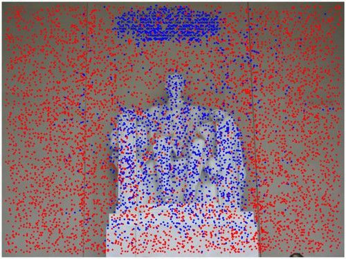
2                                                                                                                     Yuhe Jin et al.

1 Introduction                                                          cameras, in varying illumination and weather conditions
                                                                        – all of which are necessary for a comprehensive evalu-
Matching two or more views of a scene is at the core of                 ation. We reconstruct the scenes with SfM, without the
fundamental computer vision problems, including image re-               need for human intervention, providing depth maps and
trieval [54, 7, 78, 104, 70], 3D reconstruction [3, 47, 90, 122],       ground truth poses for 26k images, and reserve another
re-localization [85, 86, 57], and SLAM [68, 33, 34]. Despite            4k for a private test set.
decades of research, image matching remains unsolved in             (b) A modular pipeline incorporating dozens of methods for
the general, wide-baseline scenario. Image matching is a                feature extraction, matching, and pose estimation, both
challenging problem with many factors that need to be taken             classical and state-of-the-art, as well as multiple heuris-
into account, e.g., viewpoint, illumination, occlusions, and            tics, all of which can be swapped out and tuned sepa-
camera properties. It has therefore been traditionally ap-              rately.
proached with sparse methods – that is, with local features.        (c) Two downstream tasks – stereo and multi-view recon-
    Recent effort have moved towards holistic, end-to-end               struction – evaluated with both downstream and inter-
solutions [50, 12, 26]. Despite their promise, they are yet to          mediate metrics, for comparison.
outperform the separatists [88, 121] that are based on the          (d) A thorough study of dozens of methods and tech-
classical paradigm of step-by-step solutions. For example,              niques, both hand-crafted and learned, and their combi-
in a classical wide baseline stereo pipeline [74], one (1) ex-          nation, along with a recommended procedure for effec-
tracts local features, such as SIFT [54], (2) creates a list of         tive hyper-parameter selection.
tentative matches by nearest-neighbor search in descriptor
space, and (3) retrieves the pose with a minimal solver in-             The framework enables researchers to evaluate how a
side a robust estimator, such as the 7-point algorithm [45]         new approach performs in a standardized pipeline, both
in a RANSAC loop [40]. To build a 3D reconstruction out             against its competitors, and alongside state-of-the-art solu-
of a set of images, same matches are fed to a bundle ad-            tions for other components, from which it simply cannot be
justment pipeline [44, 106] to jointly optimize the camera          detached. This is crucial, as true performance can be easily
intrinsics, extrinsics, and 3D point locations. This modular        hidden by sub-optimal hyperparameters.
structure simplifies engineering a solution to the problem
and allows for incremental improvements, of which there
have been hundreds, if not thousands.                               2 Related Work
    New methods for each of the sub-problems, such as fea-
                                                                    The literature on image matching is too vast for a thorough
ture extraction and pose estimation, are typically studied in
                                                                    overview. We cover relevant methods for feature extraction
isolation, using intermediate metrics, which simplifies their
                                                                    and matching, pose estimation, 3D reconstruction, applica-
evaluation. However, there is no guarantee that gains in one
                                                                    ble datasets, and evaluation frameworks.
part of the pipeline will translate to the final application, as
these components interact in complex ways. For example,
patch descriptors, including very recent work [46, 110, 103,
                                                                    2.1 Local features
67], are often evaluated on Brown’s seminal patch retrieval
database [24], introduced in 2007. They show dramatic im-
                                                                    Local features became a staple in computer vision with the
provements – up to 39x relative [110] – over handcrafted
                                                                    introduction of SIFT [54]. They typically involve three dis-
methods such as SIFT, but it is unclear whether this remains
                                                                    tinct steps: keypoint detection, orientation estimation, and
true on real-world applications. In fact, we later demonstrate
                                                                    descriptor extraction. Other popular classical solutions are
that the gap narrows dramatically when decades-old base-
                                                                    SURF [18], ORB [83], and AKAZE [5].
lines are properly tuned.
                                                                         Modern descriptors often train deep networks on
    We posit that it is critical to look beyond intermedi-
                                                                    pre-cropped patches, typically from SIFT keypoints
ate metrics and focus on downstream performance. This
                                                                    (i.e.Difference of Gaussians or DoG). They include Deep-
is particularly important now as, while deep networks are
                                                                    desc [94], TFeat [13], L2-Net [102], HardNet [62], SOS-
reported to outperform algorithmic solutions on classical,
                                                                    Net [103], and LogPolarDesc [39] – most of them are
sparse problems such as outlier filtering [114, 79, 117, 97,
                                                                    trained on the same dataset [24]. Recent works leverage ad-
22], bundle adjustment [99, 93], SfM [109, 111] and SLAM
                                                                    ditional cues, such as geometry or global context, including
[100,51], our findings in this paper suggest that this may not
                                                                    GeoDesc [56] and ContextDesc [55]. There have been mul-
always be the case. To this end, we introduce a benchmark
                                                                    tiple attempts to learn keypoint detectors separately from
for wide-baseline image matching, including:
                                                                    the descriptor, including TILDE [108], TCDet [119], Quad-
(a) A dataset with thousands of phototourism images of 25           Net [89], and Key.Net [16]. An alternative is to treat this as
    landmarks, taken from diverse viewpoints, with different        an end-to-end learning problem, a trend that started with the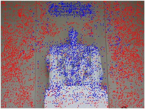
Image Matching Across Wide Baselines: From Paper to Practice                                                                                   3

     (a)            (b)            (c)           (d)          (e)            (f)             (g)           (h)          (i)            (j)
Fig. 2 On the limitations of previous datasets. To highlight the need for a new benchmark, we show examples from datasets and benchmarks
featuring posed images that have been previously used to evaluate local features and robust matchers (some images are cropped for the sake of
presentation). From left to right: (a) VGG Oxford [60], (b) HPatches [11], (c) Edge Foci [123], (d) Webcam [108], (e) AMOS [48], (f) Kitti [42],
(g) Strecha [95], (h) SILDa [10], (i) Aachen [85], (j) Ours. Notice that many (a-e) contain only planar structures or illumination changes, which
makes it easy – or trivial – to obtain ground truth poses, encoded as homographies. Other datasets are small – (g) contains very accurate depth
maps, but only two scenes and 19 images total – or do not contain a wide enough range of photometric and viewpoint transformations. Aachen (i)
is closer to ours (j), but relatively small, limited to one scene, and focused on re-localization on the day vs. night use-case.

introduction of LIFT [113] and also includes DELF [70],                   2.4 Datasets and benchmarks
SuperPoint [34], LF-Net [71], D2-Net [37] and R2D2 [81].
                                                                          Early works on local features and robust matchers typically
                                                                          relied on the Oxford dataset [60], which contains 48 im-
2.2 Robust matching                                                       ages and ground truth homographies. It helped establish two
                                                                          common metrics for evaluating local feature performance:
Inlier ratios in wide-baseline stereo can be below 10% –
                                                                          repeatability and matching score. Repeatability evaluates the
and sometimes even lower. This is typically approached
                                                                          keypoint detector: given two sets of keypoints over two im-
with iterative sampling schemes based on RANSAC [40],
                                                                          ages, projected into each other, it is defined as the ratio of
relying on closed-form solutions for pose solving such as
                                                                          keypoints whose support regions’ overlap is above a thresh-
the 5- [69], 7- [45] or 8-point algorithm [43]. Improve-
                                                                          old. The matching score (MS) is similarly defined, but also
ments to this classical framework include local optimiza-
                                                                          requires their descriptors to be nearest neighbours. Both re-
tion [28], using likelihood instead of reprojection (MLE-
                                                                          quire pixel-to-pixel correspondences – i.e., features outside
SAC) [105], speed-ups using probabilistic sampling of hy-
                                                                          valid areas are ignored.
potheses (PROSAC) [27], degeneracy check using homogra-
                                                                              A modern alternative to Oxford is HPatches [11], which
phies (DEGENSAC) [30], Graph Cut as a local optimization
                                                                          contains 696 images with differences in illumination or
(GC-RANSAC) [14], and auto-tuning of thresholds using
                                                                          viewpoint – but not both. However, the scenes are planar,
confidence margins (MAGSAC) [15].
                                                                          without occlusions, limiting its applicability.
    As an alternative direction, recent works, starting with
                                                                              Other datasets that have been used to evaluate local fea-
CNe (Context Networks) in [114], train deep networks for
                                                                          tures include DTU [1], Edge Foci [123], Webcam [108],
outlier rejection taking correspondences as input, often fol-
                                                                          AMOS [75], and Strecha’s [95]. They all have limitations
lowed by a RANSAC loop. Follow-ups include [79, 120, 97,
                                                                          – be it narrow baselines, noisy ground truth, or a small num-
117]. Differently from RANSAC solutions, they typically
                                                                          ber of images. In fact, most learned descriptors have been
process all correspondences in a single forward pass, with-
                                                                          trained and evaluated on [25], which provides a database of
out the need to iteratively sample hypotheses. Despite their
                                                                          pre-cropped patches with correspondence labels, and mea-
promise, it remains unclear how well they perform in real-
                                                                          sures performance in terms of patch retrieval. While this
world settings, compared to a well-tuned RANSAC.
                                                                          seminal dataset and evaluation methodology helped devel-
                                                                          oped many new methods, it is not clear how results translate
2.3 Structure from Motion (SfM)                                           to different scenarios – particularly since new methods out-
                                                                          perform classical ones such as SIFT by orders of magnitude,
In SfM, one jointly optimizes the location of the 3D points               which suggests overfitting.
and the camera intrinsics and extrinsics. Many improve-                       Datasets used for navigation, re-localization, or SLAM,
ments have been proposed over the years [3, 47, 31, 41, 122].             in outdoor environments are also relevant to our problem.
The most popular frameworks are VisualSFM [112] and                       These include KITTI [42], Aachen [87], Robotcar [58],
COLMAP [90] – we rely on the latter, to both generate the                 and CMU seasons [86, 9]. However, they do not feature the
ground truth and as the backbone of our multi-view task.                  wide range of transformations present in phototourism data.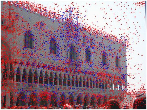
4                                                                                                                      Yuhe Jin et al.

Fig. 3 The Image Matching Challenge PhotoTourism (IMC-PT) dataset. We show a few selected images from our dataset and their corre-
sponding depth maps, with occluded pixels marked in red.

Megadepth [53] is a more representative, phototourism-                  Our approach is to obtain a ground truth signal using re-
based dataset, which using COLMAP, as in our case – it              liable, off-the-shelf technologies, while making the problem
could, in fact, easily be folded into ours.                         as easy as possible – and then evaluate new technologies on
    Benchmarks, by contrast, are few and far between – they         a much harder problem, using only a subset of that data. For
include VLBenchmark [49], HPatches [11], and SILDa [10]             example, we reconstruct a scene with hundreds or thousands
– all limited in scope. A large-scale benchmark for SfM             of images with vanilla COLMAP and then evaluate “mod-
was proposed in [91], which built 3D reconstructions with           ern” features and matchers against its poses using only two
different local features. However, only a few scenes con-           images (“stereo”) or up to 25 at a time (“multiview” with
tain ground truth, so most of their metrics are qualitative         SfM). For a discussion regarding the accuracy of our ground
– e.g.number of observations or average reprojection error.         truth data, please refer to Section 3.3.
Yi et al. [114] and Bian et al. [21] evaluate different meth-           In addition to point clouds, COLMAP provides dense
ods for pose estimation on several datasets – however, few          depth estimates. These are noisy, and have no notion of oc-
methods are considered and they are not carefully tuned.            clusions – a depth value is provided for every pixel. We
    We highlight some of these datasets/benchmarks, and             remove occluded pixels from depth maps using the recon-
their limitations, in Fig. 2. We are, to the best of our knowl-     structed model from COLMAP; see Fig. 3 for examples. We
edge, the first to introduce a public, modular benchmark for        rely on these “cleaned” depth maps to compute classical,
3D reconstruction with sparse methods using downstream              pixel-wise metrics – repeatability and matching score. We
metrics, and featuring a comprehensive dataset with a large         find that some images are flipped 90◦ , and use the recon-
range of image transformations.                                     structed pose to rotate them – along with their poses – so
                                                                    they are roughly ‘upright’, which is a reasonable assump-
                                                                    tion for this type of data.
3 The Image Matching Challenge PhotoTourism Dataset

While it is possible to obtain very accurate poses and depth        3.1 Dataset details
maps under controlled scenarios with devices like LIDAR,
this is costly and requires a specific set-up that does not scale   Out of the 25 scenes, containing almost 30k registered im-
well. For example, Strecha’s dataset [95] follows that ap-          ages in total, we select 2 for validation and 9 for testing. The
proach but contains only 19 images. We argue that a truly           remaining scenes can be used for training, if so desired, and
representative dataset must contain a wider range of trans-         are not used in this paper. We provide images, 3D recon-
formations – including different imaging devices, time of           structions, camera poses, and depth maps, for every train-
day, weather, partial occlusions, etc. Phototourism images          ing and validation scene. For the test scenes we release only
satisfy this condition and are readily available.                   a subset of 100 images and keep the ground truth private,
    We thus build on 25 collections of popular landmarks            which is an integral part of the Image Matching Challenge.
originally selected in [47, 101], each with hundreds to thou-       Results on the private test set can be obtained by sending
sands of images. Images are downsampled with bilinear in-           submissions to the organizers, who process them.
terpolation to a maximum size of 1024 pixels along the long-             The scenes used for training, validation and test are
side and their poses were obtained with COLMAP [90],                listed in Table 1, along with the acronyms used in several
which provides the (pseudo) ground truth. We do exhaustive          figures. For the validation experiments – Sections 5 and 7 –
image matching before Bundle Adjustment – unlike [92],              we choose two of the larger scenes, “Sacre Coeur” and “St.
which uses only 100 pairs for each image – and thus pro-            Peter’s Square”, which in our experience provide results that
vide enough matching images for any conventional SfM to             are quite representative of what should be expected on the
return near-perfect results in standard conditions.                 Image Matching Challenge Dataset. These two subsets have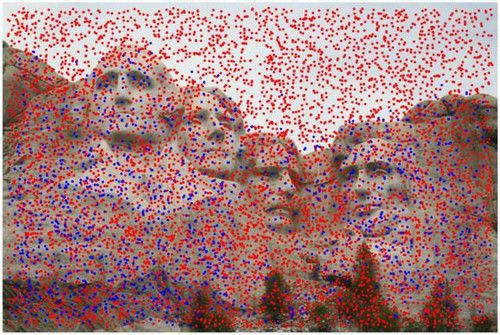
Image Matching Across Wide Baselines: From Paper to Practice 5
Name Group Images 3D points Co-visibility histogram
SC
“Brandenburg Gate” T 1363 100040
“Buckingham Palace” T 1676 234052
“Colosseum Exterior” T 2063 259807
SPS
“Grand Place Brussels” T 1083 229788
“Hagia Sophia Interior” T 888 235541
BM
“Notre Dame Front Facade” T 3765 488895
“Palace of Westminster” T 983 115868
“Pantheon Exterior” T 1401 166923
FCS
“Prague Old Town Square” T 2316 558600
“Reichstag” T 75 17823
LMS
“Taj Mahal” T 1312 94121
“Temple Nara Japan” T 904 92131
“Trevi Fountain” T 3191 580673
LB
“Westminster Abbey” T 1061 198222
“Sacre Coeur” (SC) V 1179 140659
MC
“St. Peter’s Square” (SPS) V 2504 232329
Total T + V 25.7k 3.6M
MR
“British Museum” (BM) E 660 73569
“Florence Cathedral Side” (FCS) E 108 44143
PSM
“Lincoln Memorial Statue” (LMS) E 850 58661
“London (Tower) Bridge” (LB) E 629 72235
“Milan Cathedral” (MC) E 124 33905
SF
“Mount Rushmore” (MR) E 138 45350
“Piazza San Marco” (PSM) E 249 95895
SPC
“Sagrada Familia” (SF) E 401 120723
“St. Paul’s Cathedral” (SPC) E 615 98872
AVG
Total E 3774 643k
]
]
]
]
]
]
]
]
]
]
.1
.2
.3
.4
.5
.6
.7
.8
.9
.0
,0
,0
,0
,0
,0
,0
,0
,0
,0
,1
Table 1 Scenes in the IMC-PT dataset. We provide some statistics
.0
.1
.2
.3
.4
.5
.6
.7
.8
.9
[0
[0
[0
[0
[0
[0
[0
[0
[0
[0
for the training (T), validation (V), and test (E) scenes.
Fig. 4 Co-visibility histogram. We break down the co-visibility mea-
sure for each scene in the validation (green) and test (red) sets, as well
as the average (purple). Notice how the statistics may vary significantly
been released, so that the validation results are reproducible from scene to scene.
and comparable. They can all be downloaded from the chal-
lenge website2 .
For stereo, the minimum co-visibility threshold is set to
0.1. For the multi-view task, subsets where at least 100 3D
points are visible in each image, are selected, as in [114,
3.2 Estimating the co-visibility between two images 117]. We find that both criteria work well in practice.
When evaluating image pairs, one has to be sure that two
given images share a common part of the scene – they may 3.3 On the quality of the “ground-truth”
be registered by the SfM reconstruction without having any
pixels in common as long as other images act as a ‘bridge’ Our core assumption is that accurate poses can be obtained
between them. Co-visible pairs of images are determined from large sets of images without human intervention. Such
with a simple heuristic. 3D model points, detected in both poses are used as the “ground truth” for evaluation of im-
the considered images, are localised in 2D in each image. age matching performance on pairs or small subsets of im-
The bounding box around the keypoints is estimated. The ages – a harder, proxy task. Should this assumption hold, the
ratio of the bounding box area and the whole image is the (relative) poses retrieved with a large enough number of im-
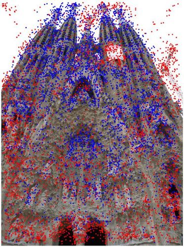
“visibility” of image i in j and j in i respectively; see Fig. 5 ages would not change as more images are added, and these
for examples. The minimum of the two “visibilities” is the poses would be the same regardless of which local feature is
“co-visibility” ratio vi,j ∈ [0, 1], which characterizes how used. To validate this, we pick the scene “Sacre Coeur” and
challenging matching of the particular image pair is. The compute SfM reconstructions with a varying number of im-
co-visibility varies significantly from scene to scene. The ages: 100, 200, 400, 800, and 1179 images (the entire “Sacre
histogram of co-visibilities is shown in Fig. 4, providing in- Coeur” dataset), where each set contains the previous one;
sights into how “hard” each scene is – without accounting new images are being added and no images are removed.
for some occlusions. We run each reconstruction three times, and report the aver-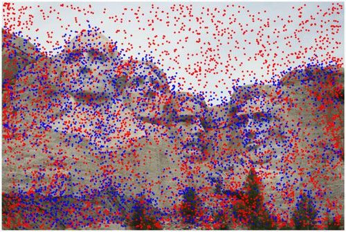
6                                                                                                                                                        Yuhe Jin et al.

Fig. 5 Co-visibility examples – image pairs from validation scenes “Sacre Coeur” (top) and “St. Peter’s Square” (bottom). Image keypoints that
are part of the 3D reconstruction are blue if they are co-visible in both images, are red otherwise. The bounding box of the co-visible points, used
to compute a per-image co-visibility ratio, is shown in blue. The co-visibility value for the image pair is the lower of these two values. Examples
include different ‘difficulty’ levels. All of the pairs are used in the evaluation except the top-right one, as we set a cut-off at 0.1.

                                        Number of Images                                                                    Number of images
       Local featured type                                                   Local feature type
                                100       200     400      800      all                                100 vs. all       200 vs. all       400 vs. all       800 vs. all
       SIFT [54]                0.06◦    0.09◦   0.06◦     0.07◦   0.09◦     SIFT [54]                0.58◦   / 0.22◦   0.31◦   / 0.08◦   0.23◦   / 0.05◦   0.18◦   / 0.04◦
       SIFT (Upright) [54]      0.07◦    0.07◦   0.04◦     0.06◦   0.09◦     SIFT (Upright) [54]      0.52◦   / 0.16◦   0.29◦   / 0.08◦   0.22◦   / 0.05◦   0.16◦   / 0.03◦
       HardNet (Upright) [62]   0.06◦    0.06◦   0.06◦     0.04◦   0.05◦     HardNet (Upright) [62]   0.35◦   / 0.10◦   0.33◦   / 0.08◦   0.23◦   / 0.06◦   0.14◦   / 0.04◦
       SuperPoint [34]          0.31◦    0.25◦   0.33◦     0.19◦   0.32◦     SuperPoint [34]          1.22◦   / 0.71◦   1.11◦   / 0.67◦   1.08◦   / 0.48◦   0.74◦   / 0.38◦
       R2D2 [80]                0.12◦    0.08◦   0.07◦     0.08◦   0.05◦     R2D2 [80]                0.49◦   / 0.14◦   0.32◦   / 0.10◦   0.25◦   / 0.08◦   0.18◦   / 0.05◦

Table 2 Standard deviation of the pose difference of three                  Table 3 Pose convergence in SfM. We report the mean/median of
COLMAP runs with different number of images. Most of them are               the difference (in degrees) between the poses extracted with the full set
below 0.1◦ , except for SuperPoint.                                         of 1179 images for “Sacre Coeur”, and different subsets of it, for four
                                                                            local feature methods – to keep the results comparable we only look at
                                                                            the 100 images in common across all subsets. We report the maximum
                                                                            among the angular difference between rotation matrices and translation
age result of the three runs, to account for the variance in-               vectors. The estimated poses are stable, with as little as 100 images.
side COLMAP. The standard deviation among different runs
is reported in Table 2. Note that these reconstructions are
only defined up to a scale factor – we do not know the abso-
lute scale that could be used to compare the reconstructions                present in the smallest subset, and compare how much their
against each other. That is why we use a simple, pairwise                   relative pose change with respect to their counterparts re-
metric instead. We pick all the pairs out of the 100 images                 constructed using the entire set – we do this for every subset,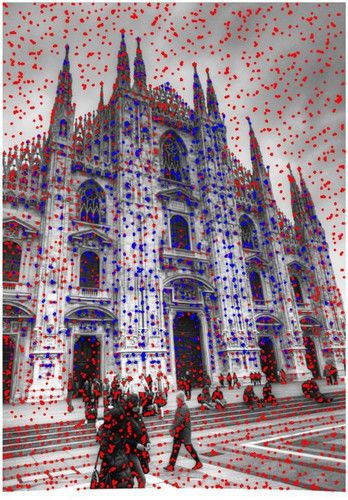
Image Matching Across Wide Baselines: From Paper to Practice                                                                                           7

                                       Compared to
  Reference
              SIFT (Upright) HardNet (Upright)    SuperPoint          R2D2
                  ◦         ◦      ◦      ◦          ◦         ◦
  SIFT [54]   0.20 / 0.05       0.26 / 0.05      1.01 / 0.62       0.26◦ / 0.09◦

Table 4 Difference between poses obtained with different local
features. We report the mean/median of the difference (in degrees)
between the poses extracted with SIFT (Upright), HardNet (Upright),
SuperPoint, or R2D2, and those extracted with SIFT. We use the max-
imum of the angular difference between rotation matrices and transla-
tion vectors. SIFT (Upright), HardNet (Upright), and R2D2 give near-
identical results to SIFT.
                                                                                          (a) SIFT              (b) SuperPoint             (c) R2D2
                                                                                   Fig. 6 COLMAP with different local features. We show the recon-
                                                                                   structed point cloud for the scene “Sacre Coeur” using three different
i.e., 100, 200, etc. Ideally, we would like the differences be-                    local features: SIFT, SuperPoint, and R2D2, using all images available
tween the relative poses to approach zero as more images are                       (1179). The reconstructions with SIFT and R2D2 are both dense, albeit
                                                                                   somewhat different. The reconstruction with SuperPoint is quite dense,
added. We list the results in Table 3, for different local fea-
                                                                                   considering it can only extract a much smaller number of features ef-
ture methods. Notice how the poses converge, especially in                         fectively, but its poses appear less accurate.
terms of the median, as more images are used, for all meth-
ods – and that the reconstructions using only 100 images are
already very stable. For SuperPoint we use a smaller number                            In addition, we note that the use of dense, ground truth
of features (2k per image), which is not enough to achieve                         depth from SfM, which is arguably less accurate that camera
pose convergence, but the error is still reduced as more im-                       poses, has been verified by multiple parties, for training and
ages are used.                                                                     evaluation, including: CNe [114], DFE [79], LF-Net [71],
                                                                                   D2-Net [37], LogPolarDesc [39], OANet [118], and Super-
     We conduct a second experiment to verify that there is                        Glue [84] among others, suggesting it is sufficiently accurate
no bias towards using SIFT features for obtaining the ground                       – several of these rely on the data used in our paper.
truth. We compare the poses obtained with SIFT to those ob-                            As a final observation, while the poses are stable, they
tained with other local features – note that our primary met-                      could still be incorrect. This can happen on highly symmet-
ric uses nothing but the estimated poses for evaluation. We                        ric structures: for instance, a tower with a square or circular
report results in Table 4. We also show the histogram of pose                      cross section. In order to prevent such errors from creeping
differences in Fig. 7. The differences in pose due to the use                      into our evaluation, we visually inspected all the images in
of different local features have a median value below 0.1◦ .                       our test set. Out of 900 of them, we found 4 misregistered
In fact, the pose variation of individual reconstructions with                     samples, all of them from the same scene, “London Bridge”,
SuperPoint is of the same magnitude as the difference be-                          which were removed from our data.
tween reconstructions from SuperPoint and other local fea-
tures: see Table 3. We conjecture that the reconstructions
with SuperPoint, which does not extract a large number of
                                                                                   4 Pipeline
keypoints, are less accurate and stable. This is further sup-
ported by the fact that the point cloud obtained with the en-
                                                                                   We outline our pipeline in Fig. 8. It takes as input N =100
tire scene generated with SuperPoint is less dense (125K 3D
                                                                                   images per scene. The feature extraction module computes
points) than the ones generated with SIFT (438K) or R2D2
                                                                                   up to K features from each image. The feature matching
(317k); see Fig. 6. In addition, we note that SuperPoint key-
                                                                                   module generates a list of putative matches for each image
points have been shown to be less accurate when it comes
                                                                                   pair, i.e. 21 N (N − 1) = 4950 combinations. These matches
to precise alignment [34, Table 4,  = 1]. Note also that the
                                                                                   can be optionally processed by an outlier pre-filtering mod-
poses from R2D2 are nearly identical to those from SIFT.
                                                                                   ule. They are then fed to two tasks: stereo, and multiview re-
    These observations reinforce our trust in the accuracy                         construction with SfM. We now describe each of these com-
of our ground truth – given a sufficient number of images,                         ponents in detail.
the choice of local feature is irrelevant, at least for the pur-
pose of retrieving accurate poses. Our evaluation considers
pose errors of up to 10◦ , at a resolution of 1◦ – significantly                   4.1 Feature extraction
smaller than the fluctuations observed here, which we con-
sider negligible. Note that these conclusions may not hold                         We consider three broad families of local features. The first
on large-scale SfM requiring loop closures, but our dataset                        includes full, “classical” pipelines, most of them handcraf-
contains landmarks, which do not suffer from this problem.                         ted: SIFT [54] (and RootSIFT [8]), SURF [18], ORB [83],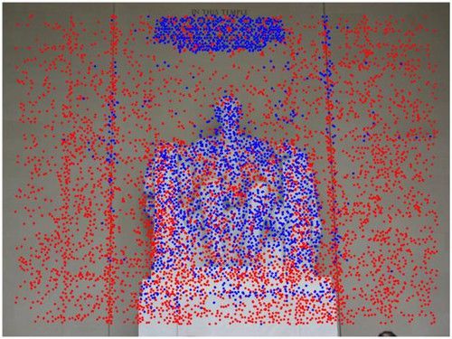
8                                                                                                                                                                        Yuhe Jin et al.

                                                Pose Difference among Different Local Features (bin width 0.2 )
             1.0 R2D2 vs. HardNet (Upright)
             80%
                                                              R2D2 vs. SIFT                 R2D2 vs. SIFT (Upright)          R2D2 vs. SuperPoint        HardNet (Upright) vs. SIFT

             0.8
             40%
    Percentage

             0.6
              0%
                 HardNet (Upright) vs. SIFT (Upright) HardNet (Upright) vs. SuperPoint       SIFT vs. SIFT (Upright)         SIFT vs. SuperPoint       SIFT (Upright) vs. SuperPoint
             0.4
             80%
             0.2
             40%
             0.0
              0%0.1 0.5 0.9 1.3 1.7 2.1 2.5 2.9 0.1 0.5 0.9 1.3 1.7 2.1 2.5 2.9 0.1 0.5 0.9 1.3 1.7 2.1 2.5 2.9 0.1 0.5 0.9 1.3 1.7 2.1 2.5 2.9 0.1 0.5 0.9 1.3 1.7 2.1 2.5 2.9
               0.0                            0.2                             0.4                            0.6                             0.8                             1.0
                                                                                         Pose Difference (degrees)
Fig. 7 Histograms of pose differences between reconstructions with different local feature methods. We consider five different local features
– including rotation-sensitive and upright SIFT – resulting in 10 combinations. The plots show that about 80% percent of image pairs are within a
0.2o pose difference, with the exception of those involving SuperPoint.

                                                                                                                        Task 1: Stereo
                                                                                                                                                    Pose Error
                                                                                                                           RANSAC
                                                                                                                                                   Computation
                             Image                 Feature                 Feature                Outlier
                             subset               Extraction               Matching             Pre-filtering          Task 2: Multi-view
                                                                                                                                                    Pose Error
                                                                                                                        SfM (Colmap)
                                                                                                                                                   Computation

                                              Full               SfM (Colmap)                Ground Truth
                                             Dataset

Fig. 8 The benchmark pipeline takes a subset of N images of a scene as input, extracts features for each, and computes matches for all M
image pairs, M = 12 N (N − 1). After an optional filtering step, the matches are fed to two different tasks. Performance is measured downstream,
by a pose-based metric, common across tasks. The ground truth is extracted once, on the full set of images.

and AKAZE [5]. We also consider FREAK [4] descrip-                                                       sults of this features are included into the Tables and Fig-
tors with BRISK [52] keypoints. We take these from                                                       ures, but not discussed in the text.
OpenCV. For all of them, except ORB, we lower the de-
tection threshold to extract more features, which increases
performance when operating with a large feature budget.
We also consider DoG alternatives from VLFeat [107]:
(VL-)DoG, Hessian [19], Hessian-Laplace [61], Harris-
                                                                                                         4.2 Feature matching
Laplace [61], MSER [59]; and their affine-covariant ver-
sions: DoG-Affine, Hessian-Affine [61, 17], DoG-AffNet
[64], and Hessian-AffNet [64].                                                                           We break this step into four stages. Given images Ii and Ij ,
                                                                                                         i 6= j, we create an initial set of matches by nearest neigh-
   The second group includes descriptors learned on DoG                                                  bor (NN) matching from Ii to Ij , obtaining a set of matches
keypoints: L2-Net [102], Hardnet [62], Geodesc [56], SOS-                                                mij . We optionally do the same in the opposite direction,
Net [103], ContextDesc [55], and LogPolarDesc [39].                                                      mji . Lowe’s ratio test [54] is applied to each list to filter
    The last group consists of pipelines learned end-to-end                                              out non-discriminative matches, with a threshold r ∈ [0, 1],
(e2e): Superpoint [34], LF-Net [71], D2-Net [37] (with both                                              creating “curated” lists m̃ij and m̃ji . The final set of pu-
single- (SS) and multi-scale (MS) variants), and R2D2 [80].                                              tative matches is lists intersection, m̃ij ∩ m̃ji = m̃∩    i↔j
    Additionally, we consider Key.Net [16], a learned detec-                                             (known in the literature as one-to-one, mutual NN, bipartite,
tor paired with HardNet and SOSNet descriptors – we pair                                                 or cycle-consistent), or union m̃ij ∪ m̃j→i = m̃∪     i↔j (sym-
it with original implementation of HardNet instead than the                                              metric). We refer to them as “both” and “either”, respec-
one provided by the authors, as it performs better3 . Post-                                              tively. We also implement a simple unidirectional matching,
IJCV update. We have added 3 more local features to the                                                  i.e., m̃ij . Finally, the distance filter is optionally applied,
benchmark after official publication of the paper – DoG-                                                 removing matches whose distance is above a threshold.
AffNet-HardNet [62,?], DoG-TFeat [13] and DoG-MKD-                                                           The “both” strategy is similar to the “symmetrical near-
Concat [66]. We take them from the kornia [38] library. Re-                                              est neighbor ratio” (sNNR) [20], proposed concurrently –
                                                                                                         SNNR combines the nearest neighbor ratio in both direc-
    3
     In [16] the models are converted to TensorFlow – we use the orig-                                   tions into a single number by taking the harmonic mean,
inal PyTorch version.                                                                                    while our test takes the maximum of the two values.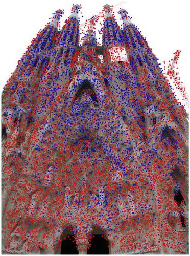
Image Matching Across Wide Baselines: From Paper to Practice                                                                  9

4.3 Outlier pre-filtering                                        4.5 Multiview task

Context Networks [114], or CNe for short, proposed a             Large-scale SfM is notoriously hard to evaluate, as it re-
method to find sparse correspondences with a permutation-        quires accurate ground truth. Since our goal is to bench-
equivariant deep network based on PointNet [77], sparking a      mark local features and matching methods, and not SfM al-
number of follow-up works [79, 32, 120, 117, 97]. We embed       gorithms, we opt for a different strategy. We reconstruct a
CNe into our framework. It often works best when paired          scene from small image subsets, which we call “bags”. We
with RANSAC [114,97], so we consider it as an optional           consider bags of 5, 10, and 25 images, which are randomly
pre-filtering step before RANSAC – and apply it to both          sampled from the original set of 100 images per scene – with
stereo and multiview. As the published model was trained         a co-visibility check. We create 100 bags for bag sizes 5, 50
on one of our validation scenes, we re-train it on “Notre        for bag size 10, and 25 for bag size 25 – i.e., 175 SfM runs
Dame Front Facade” and “Buckingham Palace”, following            in total.
CNe training protocol, i.e., with 2000 SIFT features, unidi-         We use COLMAP [90], feeding it the matches computed
rectional matching, and no ratio test. We evaluated the new      by the previous module – note that this comes before the
model on the test set and observed that its performance is       robust estimation step, as COLMAP implements its own
better than the one that was released by the authors. It could   RANSAC. If multiple reconstructions are obtained, we con-
be further improved by using different matching schemes,         sider the largest one. We also collect and report statistics
such as bidirectional matching, but we have not explored         such as the number of landmarks or the average track length.
this in this paper and leave as future work.                     Both statistics and error metrics are averaged over the three
                                                                 bag sizes, each of which is in turn averaged over its individ-
    We perform one additional, but necessary, change: CNe
                                                                 ual bags.
(like most of its successors) was originally trained to esti-
mate the Essential matrix instead of the Fundamental ma-
trix [114], i.e., it assumes known intrinsics. In order to use   4.6 Error metrics
it within our setup, we normalize the coordinates by the size
of the image instead of using ground truth calibration matri-    Since the stereo problem is defined up to a scale factor [44],
ces. This strategy has also been used in [97], and has been      our main error metric is based on angular errors. We com-
shown to work well in practice.                                  pute the difference, in degrees, between the estimated and
                                                                 ground-truth translation and rotation vectors between two
                                                                 cameras. We then threshold it over a given value for all pos-
                                                                 sible – i.e., co-visible – pairs of images. Doing so over dif-
                                                                 ferent angular thresholds renders a curve. We compute the
4.4 Stereo task
                                                                 mean Average Accuracy (mAA) by integrating this curve
                                                                 up to a maximum threshold, which we set to 10◦ – this is
The list of tentative matches is given to a robust estima-       necessary because large errors always indicate a bad pose:
tor, which estimates Fi,j , the Fundamental matrix between       30◦ is not necessarily better than 180◦ , both estimates are
Ii and Ij . In addition to (locally-optimized) RANSAC [40,       wrong. Note that by computing the area under the curve we
29], as implemented in OpenCV [23], and sklearn [72], we         are giving more weight to methods which are more accurate
consider more recent algorithms with publicly available im-      at lower error thresholds, compared to using a single value
plementations: DEGENSAC [30], GC-RANSAC [14] and                 at a certain designated threshold.
MAGSAC [15]. We use the original GC-RANSAC imple-                    This metric was originally introduced in [114], where it
mentation4 , and not the most up-to-date version, which in-      was called mean Average Precision (mAP). We argue that
corporates MAGSAC, DEGENSAC, and later changes.                  “accuracy” is the correct terminology, since we are simply
    For DEGENSAC we additionally consider disabling the          evaluating how many of the predicted poses are “correct”,
degeneracy check, which theoretically should be equiva-          as determined by thresholding over a given value – i.e., our
lent to the OpenCV and sklearn implementations – we call         problem does not have “false positives”.
this variant “PyRANSAC”. Given Fi,j , the known intrinsics           The same metric is used for multiview. Because we do
K{i,j} were used to compute the Essential matrix Ei,j , as       not know the scale of the scene a priori, it is not possible to
Ei,j = KTj Fi,j Ki . Finally, the relative rotation and trans-   measure translation error in metric terms. While we intend
lation vectors were recovered with a cheirality check with       to explore this in the future, such a metric, while more in-
OpenCV’s recoverPose.                                            terpretable, is not without problems – for instance, the range
                                                                 of the distance between the camera and the scene can vary
 4
   https://github.com/danini/graph-cut-ransac/                   drastically from scene to scene and make it difficult to com-
tree/benchmark-version                                           pare their results. To compute the mAA in pose estimation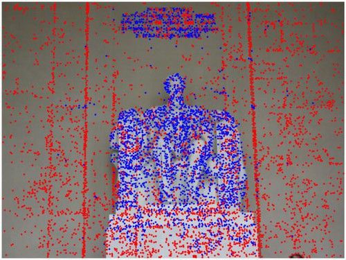
10                                                                                                                                                                                                        Yuhe Jin et al.

                                                                                                            Performance vs cost: mAA(5o )                                    Performance vs cost: mAA(10o )
for the multiview task, we take the mean of the average ac-                                      0.52                                                               0.60

curacy for every pair of cameras – setting the pose error to                                     0.50                                                               0.58

                                                                   Mean Average Accuracy (mAA)
∞ for pairs containing unregistered views. If COLMAP re-                                         0.48                                                               0.56

                                                                                                 0.46                                                               0.54
turns multiple models which cannot be co-registered (which
                                                                                                 0.44                                                               0.52
is rare) we consider only the largest of them for simplicity.
                                                                                                 0.42                                                               0.50

     For the stereo task, we can report this value for different                                 0.40                                                               0.48

co-visibility thresholds: we use v = 0.1 by default, which                                       0.38                                                               0.46

preserves most of the “hard” pairs. Note that this is not ap-                                    0.36                                                               0.44
                                                                                                   0.00    0.25    0.50   0.75   1.00   1.25   1.50   1.75   2.00     0.00   0.25    0.50   0.75   1.00   1.25   1.50   1.75   2.00
plicable to the multiview task, as all images are registered at                                                   Time in seconds (per image pair)                                  Time in seconds (per image pair)
                                                                                                          CV-RANSAC, η = 0.5 px                        PyRANSAC, η = 0.25 px                       MAGSAC, η = 1.25 px
once via bundle adjustment in SfM.                                                                        sklearn-RANSAC, η = 0.75 px                  DEGENSAC, η = 0.5 px                        GC-RANSAC, η = 0.5 px

     Finally, we consider repeatability and matching score.
                                                                   Fig. 9 Validation – Performance vs. cost for RANSAC. We evaluate
Since many end-to-end methods do not report and often do           six RANSAC variants, using 8k SIFT features with “both” matching
not have a clear measure of scale – or support region – we         and a ratio test threshold of r=0.8. The inlier threshold η and itera-
simply threshold by pixel distance, as in [82]. For the multi-     tions limit Γ are variables – we plot only the best η for each method,
view task, we also compute the Absolute Trajectory Error           for clarity, and set a budget of 0.5 seconds per image pair (dotted red
                                                                   line). For each RANSAC variant, we pick the largest Γ under this time
(ATE) [96], a metric widely used in SLAM. Since, once              “limit” and use it for all validation experiments. Computed on ‘n1-
again, the reconstructed model is scale-agnostic, we first         standard-2’ VMs on Google Compute (2 vCPUs, 7.5 GB).
scale the reconstructed model to that of the ground truth and
then compute the ATE. Note that ATE needs a minimum of
three points to align the two models.                              5 Details are Important

                                                                   Our experiments indicate that each method needs to be care-
                                                                   fully tuned. In this section we outline the methodology we
                                                                   used to find the right hyperparameters on the validation set,
4.7 Implementation                                                 and demonstrate why it is crucial to do so.

The benchmark code has been open-sourced1 along with
every method used in the paper5 . The implementation re-
                                                                   5.1 RANSAC: Leveling the field
lies on SLURM [115] for scalable job scheduling, which is
compatible with our supercomputer clusters – we also pro-          Robust estimators are, in our experience, the most sensitive
vide on-the-cloud, ready-to-go images6 . The benchmark can         part of the stereo pipeline, and thus the one we first turn to.
also run on a standard computer, sequentially. It is com-          All methods considered in this paper have three parameters
putationally expensive, as it requires matching about 45k          in common: the confidence level in their estimates, τ ; the
image pairs. The most costly step – leaving aside feature          outlier (epipolar) threshold, η; and the maximum number of
extraction, which is very method-dependent – is typically          iterations, Γ . We find the confidence value to be the least
feature matching: 2–6 seconds per image pair7 , depending          sensitive, so we set it to τ = 0.999999.
on descriptor size. Outlier pre-filtering takes about 0.5–0.8
                                                                        We evaluate each method with different values for Γ
seconds per pair, excluding some overhead to reformat the
                                                                   and η, using reasonable defaults: 8k SIFT features with bidi-
data into its expected format. RANSAC methods vary be-
                                                                   rectional matching with the “both” strategy and a ratio test
tween 0.5–1 second – as explained in Section 5 we limit
                                                                   threshold of 0.8. We plot the results in Fig. 9, against their
their number of iterations based on a compute budget, but
                                                                   computational cost – for the sake of clarity we only show
the actual cost depends on the number of matches. Note that
                                                                   the curve corresponding to the best reprojection threshold η
these values are computed on the validation set – for the test
                                                                   for each method.
set experiments we increase the RANSAC budget, in order
                                                                        Our aim with this experiment is to place all methods on
to remain compatible with the rules of the Image Matching
                                                                   an “even ground” by setting a common budget, as we need
Challenge2 . We find COLMAP to vary drastically between
                                                                   to find a way to compare them. We pick 0.5 seconds, where
set-ups. New methods will be continuously added, and we
                                                                   all methods have mostly converged. Note that these are dif-
welcome contributions to the code base.
                                                                   ferent implementations and are obviously not directly com-
 5
                                                                   parable to each other, but this is a simple and reasonable
    https://github.com/vcg-uvic/
                                                                   approach. We set this budget by choosing Γ as per Fig. 9,
image-matching-benchmark-baselines
  6
    https://github.com/etrulls/slurm-gcp                           instead of actually enforcing a time limit, which would not
  7
    Time measured on ‘n1-standard-2’ VMs on Google Cloud Com-      be comparable across different set-ups. Optimal values for
pute: 2 vCPUs with 7.5 GB of RAM and no GPU.                       Γ can vary drastically, from 10k for MAGSAC to 250k for
Image Matching Across Wide Baselines: From Paper to Practice 11
STEREO: mAA(10o ) vs Inlier Threshold STEREO: mAA(10o ) MULTIVIEW: mAA(10o )
0.8
(a) PyRANSAC (b) DEGENSAC
0.7
0.7
Mean Average Accuracy (mAA)
Mean Average Accuracy (mAA)
0.6
0.6
0.5 0.5
0.4 0.4
0.3
0.3
0.2
0.2
0.1
0.1
(c) GC-RANSAC (d) MAGSAC 0.0
0.7 60 65 70 75 80 85 90 95 None 60 65 70 75 80 85 90 95 None
Ratio test r Ratio test r
Mean Average Accuracy (mAA)
0.6 CV-AKAZE CV-SURF GeoDesc LogPolarDesc VL-DoG-SIFT
CV-FREAK ContextDesc Key.Net-HardNet R2D2 (wasf-n8-big) VL-DoGAff-SIFT
CV-ORB D2-Net (MS) Key.Net-SOSNet SOSNet VL-Hess-SIFT
0.5 CV-RootSIFT D2-Net (SS) L2-Net SuperPoint (2k points) VL-HessAffNet-SIFT
CV-SIFT DoG-HardNet LF-Net (2k points)
0.4
Fig. 11 Validation – Optimal ratio test r for matching with “both”.
0.3
We evaluate bidirectional matching with the “both” strategy (the best
0.2
one), and different ratio test thresholds r, for each feature type. We
use 8k features (2k for SuperPoint and LF-Net). For stereo, we use
0.1 PyRANSAC.
0.1
5
0.22
5
0.5
5
1
1.5
2
3
4
5
7.5
10
15
20
0.1
5
0.22
5
0.5
5
1
1.5
2
3
4
5
7.5
10
15
20
0.1
0.
0.7
0.1
0.
0.7
Inlier threshold η Inlier threshold η
CV-AKAZE CV-SURF GeoDesc LogPolarDesc SuperPoint (2k)
CV-FREAK ContextDesc Key.Net-HardNet R2D2 (waf-n16) VL-DoG-SIFT
CV-ORB
CV-RootSIFT
D2-Net (MS)
D2-Net (SS)
Key.Net-SOSNet
L2-Net
R2D2 (wasf-n16)
R2D2 (wasf-n8-big)
VL-DoGAff-SIFT
VL-Hess-SIFT
test with the threshold recommended by the authors of each
CV-SIFT DoG-HardNet LF-Net (2k) SOSNet VL-HessAffNet-SIFT
feature, or a reasonable value if no recommendation exists,
Fig. 10 Validation – Inlier threshold for RANSAC, η. We determine and the “both” matching strategy – this cuts down on the
η for each combination, using 8k features (2k for LF-Net and Super- number of outliers.
Point) with the “both” matching strategy and a reasonable value for the
ratio test. Optimal parameters (diamonds) are listed in the Section 7.
PyRANSAC. MAGSAC gives the best results for this exper- 5.3 Ratio test: One feature at a time
iment, closely followed by DEGENSAC. We patch OpenCV
to increase the limit of iterations, which was hardcoded Having “frozen” RANSAC, we turn to the feature matcher
to Γ = 1000; this patch is now integrated into OpenCV. – note that it comes before RANSAC, but it cannot be eval-
This increases performance by 10-15% relative, within our uated in isolation. We select PyRANSAC as a “baseline”
budget. However, PyRANSAC is significantly better than RANSAC and evaluate different ratio test thresholds, sep-
OpenCV version even with this patch, so we use it as our arately for the stereo and multiview tasks. For this experi-
“vanilla” RANSAC instead. The sklearn implementation is ment, we use 8k features with all methods, except for those
too slow for practical use. which cannot work on this regime – SuperPoint and LF-Net.
We find that, in general, default settings can be woefully This choice will be substantiated in Section 5.4. We report
inadequate. For example, OpenCV recommends τ = 0.99 the results for bidirectional matching with the “both” strat-
and η = 3 pixels, which results in a mAA at 10◦ of 0.3642 egy in Fig. 11, and with the “either” strategy in Fig. 12. We
on the validation set – a performance drop of 29.3% relative. find that “both” – the method we have used so far – performs
best overall. Bidirectional matching with the “either” strat-
egy produces many (false) matches, increasing the compu-
tational cost in the estimator, and requires very small ratio
5.2 RANSAC: One method at a time test thresholds – as low as r=0.65. Our experiments with
unidirectional matching indicate that is slightly worse, and
The last free parameter is the inlier threshold η. We expect it depends on the order of the images, so we did not explore
the optimal value for this parameter to be different for each it further.
local feature, with looser thresholds required for methods As expected, each feature requires different settings, as
operating on higher recall/lower precision, and end-to-end the distribution of their descriptors is different. We also ob-
methods trained on lower resolutions. serve that optimal values vary significantly between stereo
We report a wide array of experiments in Fig. 10 that and multiview, even though one might expect that bundle
confirm our intuition: descriptors learned on DoG keypoints adjustment should be able to better deal with outliers. We
are clustered, while others vary significantly. Optimal values suspect that this indicates that there is room for improve-
are also different for each RANSAC variant. We use the ratio ment in COLMAP’s implementation of RANSAC.12 Yuhe Jin et al.
STEREO: mAA(10o ) MULTIVIEW: mAA(10o ) STEREO (mAA(10o )): Ratio Test VS Distance Threshold
0.8 ORB FREAK AKAZE
Hamming Distance Threshold Hamming Distance Threshold Hamming Distance Threshold
16 24 32 40 48 64 16 32 64 96 128 16 32 64 96 128
0.7
Match RT: ”either”
Mean Average Accuracy (mAA)
0.4 Match RT: ”both” 0.4 0.4
Mean Average Accuracy (mAA)
0.6
Match DT: ”either”
Match DT: ”both”
0.5 0.3 0.3 0.3
0.4
0.2 0.2 0.2
0.3
0.1 0.1 0.1
0.2
0.1 0.0 0.0 0.0
0.60 0.70 0.80 0.90 None 0.60 0.70 0.80 0.90 None 0.60 0.70 0.80 0.90 None
Ratio test Ratio test Ratio test
0.0
60 65 70 75 80 85 90 95 None 60 65 70 75 80 85 90 95 None
Ratio test r Ratio test r Fig. 14 Validation – Matching binary descriptors. We filter out
CV-AKAZE CV-ORB CV-SURF GeoDesc SOSNet non-discriminative matches with the ratio test or a distance threshold.
CV-DoG/HardNet CV-RootSIFT D2-Net (MS) LF-Net (2k points) SuperPoint (2k)
CV-FREAK CV-SIFT D2-Net (SS) LogPolarDesc
The latter (the standard) performs worse in our experiments.
Fig. 12 Validation – Optimal ratio test r for matching with “ei-
ther”. Equivalent to Fig. 11 but with the “either” matching strategy. for different values of K in Fig. 13. We use PyRANSAC
This strategy requires aggressive filtering and does not reach the per-
formance of “both”, we thus explore only a subset of the methods.
with reasonable defaults for all three matching strategies,
with SIFT features.
STEREO: mAA(10o ) MULTIVIEW: mAA(10o ) As expected, performance is strongly correlated with the
0.6 number of features. We find 8k to be a good compromise be-
Mean Average Accuracy (mAA)
0.5
tween performance and cost, and also consider 2k (actually
2048) as a ‘cheaper’ alternative – this also provides a fair
0.4
comparison with some learned methods which only operate
0.3
on that regime. We choose these two values as valid cate-
0.2
Unidirectional (r =0.80) gories for the open challenge2 linked to the benchmark, and
Bidirectional + ’either’ (r =0.65)
0.1 do the same on this paper for consistency.
Bidirectional + ’both’ (r =0.80)
0.0
500 2k 4k 6k 8k 10k 12k 15k 500 2k 4k 6k 8k 10k 12k 15k
Number of features Number of features
Fig. 13 Validation – Number of features. Performance on the stereo 5.5 Additional experiments
and multi-view tasks while varying the number of SIFT features, with
three matching strategies, and reasonable defaults for the ratio test r.
Some methods require additional considerations before
evaluating them on the test set. We briefly discuss them in
Note how the ratio test is critical for performance, and this section. Further experiments are available in Section 7.
one could arbitrarily select a threshold that favours one Binary features (Fig. 14). We consider three binary de-
method over another, which shows the importance of proper scriptors: ORB [83], AKAZE [5], and FREAK [4] Binary
benchmarking. Interestingly, D2-Net is the only method that descriptor papers historically favour a distance threshold in
clearly performs best without the ratio test. It also performs place of the ratio test to reject non-discriminative matches
poorly overall in our evaluation, despite reporting state-of- [83], although some papers have used the ratio test for ORB
the-art results in other benchmarks [60, 11, 85, 98] – without descriptors [6]. We evaluate both in Fig. 14 – as before, we
the ratio test, the number of tentative matches might be too use up to 8k features and matching with the “both” strategy.
high for RANSAC or COLMAP to perform well. The ratio test works better for all three methods – we use
Additionally, we implement the first-geometric- it instead of a distance threshold for all experiments in the
inconsistent ratio threshold, or FGINN [63]. We find that paper, including those in the previous sections.
although it improves over unidirectional matching, its gains
mostly disappear against matching with “both”. We report On the influence of the detector (Fig. 15). We embed sev-
these results in Section 7.2. eral popular blob and corner detectors into our pipeline,
with OpenCV’s DoG [54] as a baseline. We combine mul-
tiple methods, taking advantage of the VLFeat library: Dif-
5.4 Choosing the number of features ference of Gaussians (DoG), Hessian [19], HessianLaplace
[61], HarrisLaplace [61], MSER [59], DoGAffine, Hessian-
The ablation tests in this section use (up to) K=8000 feature Affine [61, 17], DoG-AffNet [64], and Hessian-AffNet [64].
(2k for SuperPoint and LF-Net, as they are trained to extract We pair them with SIFT descriptors, also computed with
fewer keypoints). This number is commensurate with that VLFeat, as OpenCV cannot process affine keypoints, and
used by SfM frameworks [112, 90]. We report performance report the results in Fig. 15. VLFeat’s DoG performsImage Matching Across Wide Baselines: From Paper to Practice 13
STEREO w/ SIFT descriptors STEREO w/ SIFT descriptors
0.7 0.60 6 Establishing the State of the Art
0.6
0.58
0.5
0.56
mAA(10o )
With the findings and the optimal parameters found in Sec-
mAA(10o )
0.4
0.54
0.3
0.52
tion 5, we move on to the test set, evaluating many meth-
0.2
0.1 0.50 ods with their optimal settings. All experiments in this
0.0 0.48 section use bidirectional matching with the ‘’both” strat-
oG
oG
n
p
p
R
oG
oG
e
et
+A ian
+A e
et
a
La
La
n
n
SE
ffN
ffN
si
ffi
ffi
D
D
D
D
s
es
ar
es
M
es
+A
V-
L-
V-
L-
egy. We consider a large feature budget (up to 8k features)
+A
H
H
H
L-
H
V
C
V
C
L-
L-
L-
L-
V
V
V
V
V
Detector Affine detector
and a smaller one (up to 2k), and evaluate many detec-
Fig. 15 Validation – Benchmarking detectors. We evaluate the per- tor/descriptor combinations.
formance on the stereo task while pairing different detectors with SIFT
descriptors. The dashed, black line indicates OpenCV SIFT – the base-
We make three changes with respect to the validation ex-
line. Left: OpenCV DoG vs. VLFeat implementations of blob detec- periments of the previous section. (1) We double the RAN-
tors (DoG, Hessian, HesLap) and corner detectors (Harris, HarLap), SAC budget from 0.5 seconds (used for validation) to 1 sec-
and MSER. Right: Affine shape estimation for DoG and Hessian key- ond per image pair, and adjust the maximum number of it-
points, against the plain version. We consider a classical approach,
Baumberg (Affine) [17], and the recent, learned AffNet [64] – they
erations Γ accordingly – we made this decision to encour-
provide a small but inconsistent boost. age participants to the challenge based on this benchmark to
use built-in methods rather than run RANSAC themselves to
squeeze out a little extra performance, and use the same val-
STEREO: mAA(10o ) ues in the paper for consistency. (2) We run each stereo and
multiview evaluation three times and average the results, in
Mean Average Accuracy (mAA)
0.60
order to decrease the potential randomness in the results –
0.55 in general, we found the variations within these three runs
0.50
to be negligible. (3) We use brute-force to match descriptors
instead of FLANN, as we observed a drop in performance.
0.45
For more details, see Section 6.6 and Table 12.
0.40 For stereo, we consider DEGENSAC and MAGSAC,
SIFT
which perform the best in the validation set, and PyRAN-
0.35
HardNet SAC as a ‘baseline’ RANSAC. We report the results with
6 8 12 16 20 24 both 8k features and 2k features in the following subsec-
Patch scaling factor
tions. All observations are in terms of mAA, our primary
Fig. 16 Validation – Scaling the descriptor support region. Per- metric, unless stated otherwise.
formance with SIFT and HardNet descriptors while applying a scaling
factor λ to the keypoint scale (note that OpenCV’s default value is
λ=12). We consider SIFT and HardNet. Default values are optimal or
near-optimal.
6.1 Results with 8k features — Tables 5 and 6
On the stereo task, deep descriptors extracted on DoG key-
points are at the top in terms of mAA, with SOSNet being
marginally better than OpenCV’s. Its affine version gives a #1, closely followed by HardNet. Interestingly, ‘HardNetA-
small boost. Given the small gain and the infrastructure bur- mos+’ [76], a version trained on more datasets – Brown [24],
den of interacting with a Matlab/C library, we use OpenCV’s HPatches [11], and AMOS-patches [76] – performs worse
DoG implementation for most of this paper. than the original models, trained only on the “Liberty” scene
from Brown’s dataset. On the multiview task, HardNet edges
On increasing the support region (Fig. 16). The size out ContextDesc, SOSNet and LogpolarDesc by a small
(“scale”) of the support region used to compute a descrip- margin.
tor can significantly affect its performance [36, 116, 2]. We We also pair HardNet and SOSNet with Key.Net, a
experiment with different scaling factors, using DoG with learned detector, which performs worse than with DoG
SIFT and HardNet [62], and find that 12× the OpenCV scale when extracting a large number of features, with the excep-
(the default value) is already nearly optimal, confirming the tion of Key.Net + SOSNet on the multiview task.
findings reported in [39]. We show these results in Fig. 16. R2D2, the best performing end-to-end method, does
Interestingly, SIFT descriptors do benefit from increasing well on multiview (#7), but performs worse than SIFT on
the scaling factor from 12 to 16, but the difference is very stereo – it produces a much larger number of “inliers”
small – we thus use the recommended value of 12 for the (which may be correct or incorrect) than most other meth-
rest of the paper. This, however, suggests that deep descrip- ods. This suggests that, like D2-Net, its lack of compatibil-
tors such as HardNet might be able to increase performance ity with the ratio test may be a problem when paired with
slightly by training on larger patches. sample-based robust estimators, due to a lower inlier ratio.You can also read