MonoSLAM: Real-Time Single Camera SLAM - Andrew J. Davison, Ian D. Reid, Nicholas D. Molton and Olivier Stasse
←
→
Page content transcription
If your browser does not render page correctly, please read the page content below

1

      MonoSLAM: Real-Time Single Camera SLAM
          Andrew J. Davison, Ian D. Reid, Nicholas D. Molton and Olivier Stasse

                                                             Abstract
           We present a real-time algorithm which can recover the 3D trajectory of a monocular camera, moving rapidly
      through a previously unknown scene. Our system, which we dub MonoSLAM, is the first successful application of
      the SLAM methodology from mobile robotics to the ‘pure vision’ domain of a single uncontrolled camera, achieving
      real-time but drift-free performance inaccessible to Structure from Motion approaches. The core of the approach is
      the on-line creation of a sparse but persistent map of natural landmarks within a probabilistic framework. Our key
      novel contributions include an active approach to mapping and measurement, the use of a general motion model
      for smooth camera movement, and solutions for monocular feature initialization and feature orientation estimation.
      Together, these add up to an extremely efficient and robust algorithm which runs at 30Hz with standard PC and
      camera hardware.
           This work extends the range of robotic systems in which SLAM can be usefully applied, but also opens up
      new areas. We present applications of MonoSLAM to real-time 3D localization and mapping for a high-performance
      full-size humanoid robot, and live augmented reality with a hand-held camera.

                                                           Index Terms
          I.2.9.a Autonomous vehicles, I.2.10.a 3D/stereo scene analysis, I.4.8.n Tracking

                                               I. I NTRODUCTION
   The last ten years have seen significant progress in autonomous robot navigation, and specifically
SLAM (Simultaneous Localization and Mapping) has become well defined in the robotics community
as the question of a moving sensor platform constructing a representation of its environment on the fly
while concurrently estimating its ego-motion. SLAM is today is routinely achieved in experimental robot
systems using modern methods of sequential Bayesian inference, and SLAM algorithms are now starting
to cross over into practical systems. Interestingly however, and despite the large computer vision research
community, until very recently the use of cameras has not been at the center of progress in robot SLAM,
with much more attention given to other sensors such as laser range-finders and sonar.
   This may seem surprising since for many reasons vision is an attractive choice of SLAM sensor: cameras
are compact, accurate, non-invasive and well-understood — and today cheap and ubiquitous. Vision of
course also has great intuitive appeal as the sense humans and animals primarily use to navigate. However,
cameras capture the world’s geometry only indirectly through photometric effects, and it was thought too
difficult to turn the sparse sets of features popping out of an image into reliable long-term maps generated
in real-time, particularly since the data rates coming from a camera are so much higher than those from
other sensors.
   Instead, vision researchers concentrated on reconstruction problems from small image sets, developing
the field known as Structure from Motion (SFM). SFM algorithms have been extended to work on
longer image sequences, (e.g. [1]–[3]), but these systems are fundamentally off-line in nature, analyzing
a complete image sequence to produce a reconstruction of the camera trajectory and scene structure
observed. To obtain globally consistent estimates over a sequence, local motion estimates from frame-to-
frame feature matching are refined in a global optimization moving backwards and forwards through the
   A. J. Davison (corresponding author) is with the Department of Computing, Imperial College, 180 Queen’s Gate, SW7 2AZ, London,
UK. Email: ajd@doc.ic.ac.uk.
   I. D. Reid is with the Robotics Research Group, Department of Engineering Science, University of Oxford, OX1 3PJ, UK. Email:
ian@robots.ox.ac.uk.
   N. D. Molton is with Imagineer Systems Ltd., The Surrey Technology Centre, 40 Occam Road, The Surrey Research Park, Guildford
GU2 7YG, UK. Email: ndm@imagineersystems.com
   O. Stasse is with the Joint Japanese-French Robotics Laboratory (JRL), CNRS/AIST, AIST Central 2, 1-1-1 Umezono, Tsukuba, 305-8568
Japan. Email: olivier.stasse@aist.go.jp.
2

whole sequence (called bundle adjustment). These methods are perfectly suited to the automatic analysis of
short image sequences obtained from arbitrary sources — movie shots, consumer video or even decades-old
archive footage — but do not scale to consistent localization over arbitrarily long sequences in real-time.
   Our work is highly focused on high frame-rate real-time performance (typically 30Hz) as a requirement.
In applications, real-time algorithms are necessary only if they are to be used as part of a loop involving
other components in the dynamic world — a robot that must control its next motion step, a human that
needs visual feedback on his actions or another computational process which is waiting for input. In these
cases, the most immediately useful information to be obtained from a moving camera in real-time is where
it is, rather than a fully detailed ‘final result’ map of a scene ready for display. Although localization and
mapping are intricately coupled problems, and it has been proven in SLAM research that solving either
requires solving both, in this work we focus on localization as the main output of interest. A map is
certainly built, but it is a sparse map of landmarks optimized towards enabling localization.
   Further, real-time camera tracking scenarios will often involve extended and looping motions within a
restricted environment (as a humanoid performs a task, a domestic robot cleans a home, or room is viewed
from different angles with graphical augmentations). Repeatable localization, in which gradual drift from
ground truth does not occur, will be essential here, and much more important than in cases where a
moving camera continually explores new regions without returning. This is where our fully-probabilistic
SLAM approach comes into its own: it will naturally construct a persistent map of scene landmarks to
be referenced indefinitely in a state-based framework, and permit loop closures to correct long-term drift.
Forming a persistent world map means that if camera motion is restricted, the processing requirement
of the algorithm is bounded and continuous real-time operation can be maintained, unlike in tracking
approaches such as [4] where loop-closing corrections are achieved by matching to a growing history of
past poses.

A. Contributions of this Paper
   Our key contribution is to show that it is indeed possible to achieve real-time localization and mapping
with a single freely moving camera as the only data source. We achieve this by applying the core of
the probabilistic SLAM methodology with novel insights specific to what here is a particularly difficult
SLAM scenario. The MonoSLAM algorithm we explain and demonstrate achieves the efficiency required
for real-time operation by using an active, guided approach to feature mapping and measurement, a general
motion model for smooth 3D camera movement to capture the dynamical prior information inherent in a
continuous video stream, and a novel top-down solution to the problem of monocular feature initialization.
   In a nutshell, when compared to SFM approaches to sequence analysis, using SLAM we are able
both to implement on-the-fly probabilistic estimation of the state of the moving camera and its map, and
benefit from this in using the running estimates to guide efficient processing. This aspect of SLAM is
often overlooked. Sequential SLAM is very naturally able for instance to select a set of highly salient and
trackable but efficiently spaced features to put into its visual map, with the use of only simple mapping
heuristics. Sensible confidence bound assumptions allow all but the most important image processing to
be avoided, and at high frame-rates all but tiny search regions of incoming images are completely ignored
by our algorithm. Our approach to mapping can be summarized as ‘a sparse map of high quality features’.
   We are able in this paper to demonstrate real-time MonoSLAM indoors in room-sized domains. A long
term goal in SLAM shared by many would be to achieve a system with the following performance: a
single low-cost camera attached to a portable computer would be switched on at an arbitrary location
in an unknown scene, then carried off by a fast-moving robot (perhaps flying, or jumping) or even a
running human through an arbitrarily large domain, all the time effortlessly recovering its trajectory in
real-time and building a detailed, persistent map of all it has seen. While others attack the large map
issue, but continue to work with the same slow-moving robots and multi-sensor platforms as before,
we are approaching the problem from the other direction and solve issues relating to highly dynamic
3D motion, commodity vision-only sensing, processing efficiency and relaxing platform assumptions. We
believe that our results are of both theoretical and practical importance because they open up completely
new avenues for the application of SLAM techniques.
3

   The current paper draws on earlier work published in conference papers [5]–[7]. We also present new
unpublished results demonstrating the advanced use of the algorithm in humanoid robotics and augmented
reality applications.

                                            II. R ELATED W ORK
   The work of Harris and Pike [8], whose DROID system built visual maps sequentially using input from
a single camera, is perhaps the grandfather of our research and was far ahead of its time. Impressive
results showed 3D maps of features from long image sequences, and a later real-time implementation was
achieved. A serious oversight of this work, however, was the treatment of the locations of each of the
mapped visual features as uncoupled estimation problems, neglecting the strong correlations introduced by
the common camera motion. Closely-related approaches were presented by Ayache [9] and later Beardsley
et al. [10] in an uncalibrated geometrical framework, but these approaches also neglected correlations, the
result being over-confident mapping and localization estimates and an inability to close loops and correct
drift.
   Smith et al. [11] and at a similar time Moutarlier and Chatila [12] had proposed taking account of all
correlations in general robot localization and mapping problems within a single state vector and covariance
matrix updated by the Extended Kalman Filter (EKF). Work by Leonard [13], Manyika [14] and others
demonstrated increasingly sophisticated robot mapping and localization using related EKF techniques,
but the single state vector and ‘full covariance’ approach of Smith et al. did not receive widespread
attention until the mid to late nineties, perhaps when computing power reached the point where it could
be practically tested. Several early implementations [15]–[19] proved the single EKF approach for building
modest-sized maps in real robot systems, and demonstrated convincingly the importance of maintaining
estimate correlations. These successes gradually saw very widespread adoption of the EKF as the core
estimation technique in SLAM, and its generality as a Bayesian solution was understood across a variety
of different platforms and sensors.
   In the intervening years, SLAM systems based on the EKF and related probabilistic filters have
demonstrated impressive results in varied domains. The methods deviating from the standard EKF have
mainly aimed at building large scale maps, where the EKF suffers problems of computational complexity
and inaccuracy due to linearization, and have included sub-mapping strategies (e.g. [20], [21]) and
factorized particle filtering (e.g. [22]). The most impressive results in terms of mapping accuracy and
scale have come from robots using laser range-finder sensors. These directly return accurate range and
bearing scans over a slice of the nearby scene, which can either be processed to extract repeatable features
to insert into a map (e.g. [23]) or simply matched whole-scale with other overlapping scans to accurately
measure robot displacement and build a map of historic robot locations each with a local scan reference
(e.g. [24], [25]).

A. Vision-Based SLAM
  Our algorithm uses vision as the only outward-looking sense. In the introduction we mentioned the
additional challenges posed by vision over laser sensors, which include the very high input data rate, the
inherent 3D quality of visual data, the lack of direct depth measurement and the difficulty in extracting
long-term features to map. These factors have combined to mean that there have been relatively few
successful vision-only SLAM systems (where now we define a SLAM system as one able to construct
persistent maps on the fly while closing loops to correct drift). In this section we review some of the
most interesting and place our work into context.
  Neira et al. presented a simple system mapping vertical line segments in 2D in a constrained indoor
environment [26], but the direct ancestor of the approach in the current paper was the work by Davison
and Murray [18], [27], [28] whose system using fixating active stereo was the first visual SLAM system
with processing in real-time (at 5Hz), able to build a 3D map of natural landmarks on the fly and control a
mobile robot. The robotic active head that was used forced a one-by-one choice of feature measurements
and sparse mapping. Nevertheless, it was proved that a small set of landmarks could provide a very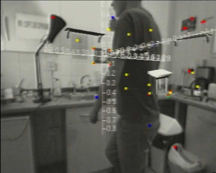
4

accurate SLAM reference if carefully chosen and spread. Davison and Kita [29] extended this method to
the case of a robot able to localize while traversing non-planar ramps by combining stereo vision with
an inclinometer.
   In more recent work, vision-based SLAM has been used in a range of different systems. Jung and
Lacroix [30] presented a stereo vision SLAM system using a downward-looking stereo rig to localize
a robotic airship and perform terrain mapping. Their implementation was sequential but did not run in
real-time and relied on a wide baseline fixed stereo rig to obtain depth measurements directly. Kim and
Sukkarieh [31] used monocular vision in combination with accurate inertial sensing to map ground-based
targets from a dynamically maneuvering UAV in an impressive system, though the targets were artificially
placed and estimation of their locations is made easier by the fact that they can be assumed to lie in a
plane.
   Bosse et al. [20], [32] used omnidirectional vision in combination with other sensors in their ATLAS
sub-mapping framework, making particular use of lines in a man-made environment as consistent bearing
references. Most recently Eustice et al. [33] have used a single downward-looking camera and inertial
sensing to localize an underwater remote vehicle and produce detailed seabed reconstructions from low
frame-rate image sequences. Using an efficient sparse information filter their approach scales well to
large-scale mapping in their experimental setup where loop closures are relatively infrequent.
   Recently published work by Sim et al. [34] uses an algorithm combining SIFT features [35] and
FastSLAM filtering [22] to achieve particularly large-scale vision-only SLAM mapping. Their method
is processor-intensive, and at an average of 10 seconds processing time per frame is currently a large
factor away from real-time operation. The commercial vSLAM system [36] also uses SIFT features,
though within a SLAM algorithm which relies significantly on odometry to build a connected map of
recognizable locations rather than fully continuous accurate localization. There is little doubt that invariant
features such as SIFT provide a high level of performance in matching, and permit high fidelity ‘location
recognition’ in the same way as they were designed for use in visual object recognition. Their value in
loop-closing or for localizing a ‘lost robot’, which involve matching with very weak priors, is clear. They
are less suited to continuous tracking, however, due to the high computational cost of extracting them —
a method like ours using active search will always outperform invariant matching for speed.
   A stress of our work is to simplify the hardware required for SLAM to the simplest case possible, a
single camera connected to a computer, and to require a minimum of assumptions about this camera’s
free 3D movement. Several authors have presented real-time camera tracking systems with goals similar
to our own. McLauchlan and Murray [37] introduced the VSDF (Variable State-Dimension Filter) for
simultaneous structure and motion recovery from a moving camera using a sparse information filter
framework, but were not able to demonstrate long-term tracking or loop closing. The approach of Chiuso
et al. [38] shared several of the ideas of our work, including the propagation of map and localization
uncertainty using a single Extended Kalman Filter, but only limited results of tracking small groups of
objects with small camera motions were presented. Their method used simple gradient descent feature
tracking and was therefore unable to match features during high acceleration or close loops after periods
of neglect. Nistér [39] presented a real-time system based very much on the standard structure from
motion methodology of frame-to-frame matching of large numbers of point features which was able to
recover instantaneous motions impressively but again had no ability to re-recognize features after periods
of neglect and therefore would lead inevitably to rapid drift in augmented reality or localization. Foxlin
[40] has taken a different approach in a single camera system by using fiducial markers attached to
the ceiling in combination with high-performance inertial sensing. This system achieved very impressive
and repeatable localization results but with the requirement for substantial extra infrastructure and cost.
Burschka and Hager [41] demonstrated a small-scale visual localization and mapping system, though by
separating the localization and mapping steps they neglect estimate correlations and the ability of this
method to function over long time periods is doubtful.
   In the following section we will present our method step by step in a form accessible to readers
unfamiliar with the details of previous SLAM approaches.
5
(a) (b)
Fig. 1. (a) A snapshot of the probabilistic 3D map, showing camera position estimate and feature position uncertainty ellipsoids. In this
and other figures in the paper the feature color code is as follows: red = successfully measured; blue = attempted but failed measurement;
yellow = not selected for measurement on this step. (b) Visually salient feature patches detected to serve as visual landmarks and the 3D
planar regions deduced by back-projection to their estimated world locations. These planar regions are projected into future estimated camera
positions to predict patch appearance from new viewpoints.
III. M ETHOD
A. Probabilistic 3D Map
The key concept of our approach, as in [11], is a probabilistic feature-based map, representing at any
instant a snapshot of the current estimates of the state of the camera and all features of interest, and
crucially also the uncertainty in these estimates. The map is initialized at system start-up and persists
until operation ends, but evolves continuously and dynamically as it is updated by the Extended Kalman
Filter. The probabilistic state estimates of the camera and features are updated during camera motion and
feature observation. When new features are observed the map is enlarged with new states, and if necessary
features can also be deleted.
The probabilistic character of the map lies in the propagation over time not only of the mean ‘best’
estimates of the states of the camera and features but a first order uncertainty distribution describing the
size of possible deviations from these values. Mathematically, the map is represented by a state vector
x̂ and covariance matrix P. State vector x̂ is composed of the stacked state estimates of the camera and
features, and P is a square matrix of equal dimension which can be partitioned into sub-matrix elements
as follows:
x̂v Pxx Pxy1 Pxy2 . . .
ŷ1 P P P ...
x̂ = , P = y1 x y1 y1 y1 y2
ŷ2 Py2 x Py2 y1 Py2 y2 . . . . (1)
.. .. .. ..
. . . .
In doing this the probability distribution over all map parameters is approximated as a single multi-variate
Gaussian distribution in a space of dimension equal to the total state vector size.
Explicitly, the camera’s state vector xv comprises a metric 3D position vector rW , orientation quaternion
qRW , velocity vector vW and angular velocity vector ω R relative to a fixed world frame W and ‘robot’
frame R carried by the camera (13 parameters):
W
r
qW R
xv = vW .
(2)
ωR
In this work feature states yi are the 3D position vectors of the locations of point features. Camera and
feature geometry and coordinate frames are defined in Figure 3(a).
The role of the map is primarily to permit real-time localization rather than serve as a complete scene
description, and we therefore aim to capture a sparse set of high-quality landmarks. We assume that the
scene is rigid and that each landmark is a stationary world feature. Specifically in this work each landmark
is assumed to correspond to a well-localized point feature in 3D space. The camera is modeled as a rigid
body needing translation and rotation parameters to describe its position, and we also maintain estimates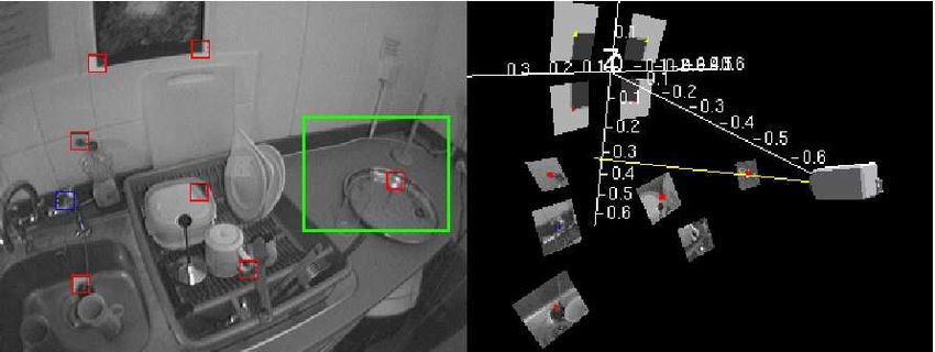
6

of its linear and angular velocity: this is important in our algorithm since we will make use of motion
dynamics as will be explained in Section III-D.
   The map can be pictured as in Figure 1(a): all geometric estimates can be considered as surrounded by
ellipsoidal regions representing uncertainty bounds (here corresponding to 3 standard deviations). What
Figure 1(a) cannot show is that the various ellipsoids are potentially correlated to various degrees: in
sequential mapping, a situation which commonly occurs is that spatially close features which are often
observed simultaneously by the camera will have position estimates whose difference (relative position)
is very well known while the position of the group as a whole relative to the global coordinate frame may
not be. This situation is represented in the map covariance matrix P by non-zero entries in the off-diagonal
matrix blocks, and comes about naturally through the operation of the algorithm.
   The total size of the map representation is order O(N 2 ) where N is the number of features, and the
complete SLAM algorithm we use has O(N 2 ) complexity. This means that the number of features which
can be maintained with real-time processing is bounded — in our system to around 100 in current 30Hz
implementation.
   There are strong reasons why we have chosen in this work to use the ‘standard’ single, full covariance
EKF approach to SLAM rather than variants which use different probabilistic representations. As we have
stated, our current goal is long-term, repeatable localization within restricted volumes. The pattern of
observation of features in one of our maps is quite different from that seen in many other implementations
of SLAM for robot mapping, such as [25], [34] or [22]. Those robots move largely through corridor-like
topologies, following exploratory paths until they infrequently come back to places they have seen before,
at that stage correcting drift around loops. Relatively ad-hoc approaches can be taken to distributing
the correction around the well-defined loops, whether this is through a chain of uncertain pose-to-pose
transformations or sub-maps, or by selecting from a potentially impoverished discrete set of trajectory
hypotheses represented by a finite number of particles.
   In our case, as a free camera moves and rotates in 3D around a restricted space, individual features will
come in and out of the field of view in varying sequences, various subsets of features at different depths
will be co-visible as the camera rotates, and loops of many different sizes and inter-linking patterns will
be routinely closed. We have considered it very important to represent the detailed, flexible correlations
which will arise between different parts of the map accurately. Within the class of known methods, this
is only computationally feasible with a sparse map of features maintained within a single state vector and
covariance matrix. 100 well-chosen features turns out to be sufficient with careful map management to
span a room. In our opinion, it remains to be proven whether a method (for instance FastSLAM [22],
[42]) which can cope with a much larger number of features but represent correlations less accurately
will be able to give such good repeatable localization results in agile single camera SLAM.

B. Natural Visual Landmarks
   Now we turn specifically to the features which make up the map. We have followed the approach
of Davison and Murray [5], [27], who showed that relatively large (11×11 pixels) image patches are
able to serve as long-term landmark features, the large templates having more unique signatures than
standard corner features. However we extend the power of such features significantly by using the camera
localization information we have available to improve matching over large camera displacements and
rotations.
   Salient image regions are originally detected automatically (at times and in locations guided by the
strategies of Section III-G) using the detection operator of Shi and Tomasi [43] from the monochrome
images obtained from the camera (note that in the current work we use monochrome images primarily for
reasons of efficiency). The goal is to be able to identify these same visual landmarks repeatedly during
potentially extreme camera motions, and therefore straightforward 2D template matching (as in [5]) is
very limiting, as after only small degrees of camera rotation and translation the appearance of a landmark
can change greatly. To improve on this, we make the approximation that each landmark lies on a locally
planar surface — an approximation that will be very good in many cases and bad in others, but a great
7

                                       (a)                                                     (b)
Fig. 2. (a) Matching the four known features of the initialization target on the first frame of tracking. The large circular search regions
reflect the high uncertainty assigned to the starting camera position estimate. (b) Visualization of the model for ‘smooth’ motion: at each
camera position we predict a most likely path together with alternatives with small deviations.

deal better than assuming that the appearance of the patch will not change at all. Further, since we do
not know the orientation of this surface, we make the assignment that the surface normal is parallel to
the vector from the feature to the camera at initialization (in Section III-H we will present a method
for updating estimates of this normal direction). Once the 3D location, including depth, of a feature
has been fully initialized using the method of Section III-F, each feature is stored as an oriented planar
texture (Figure 1(b)). When making measurements of a feature from new camera positions, its patch can
be projected from 3D to the image plane to produce a template for matching with the real image. This
template will be a warped version of the original square template captured when the feature was first
detected. In general this will be a full projective warping, with shearing and perspective distortion, since
we just send the template through backward and forward camera models. Even if the orientation of the
surface on which the feature lies is not correct, the warping will still take care successfully of rotation
about the cyclotorsion axis and scale (the degrees of freedom to which the SIFT descriptor is invariant)
and some amount of other warping.
   Note that we do not update the saved templates for features over time — since the goal is repeatable
localization, we need the ability to exactly re-measure the locations of features over arbitrarily long time
periods. Templates which are updated over time will tend to drift gradually from their initial positions.

C. System Initialization
   In most SLAM systems, the robot has no specific knowledge about the structure of the world around
it when first switched on. It is free to define a coordinate frame within which to estimate its motion and
build a map, and the obvious choice is to fix this frame at the robot’s starting position, defined as the
origin. In our single camera SLAM algorithm we choose to aid system start-up with a small amount of
prior information about the scene in the shape of a known target placed in front of the camera. This
provides several features (typically four) with known positions and of known appearance. There are two
main reasons for this:
   1) In single camera SLAM, with no direct way to measure feature depths or any odometry, starting
       from a target of known size allows us to assign a precise scale to the estimated map and motion
       — rather than running with scale as a completely unknown degree of freedom. Knowing the scale
       of the map is desirable whenever it must be related to other information such as priors on motion
       dynamics or features depths, and makes it much more easy to use in real applications.
   2) Having some features in the map right from the start means that we can immediately enter our
       normal predict-measure-update tracking sequence without any special first step. With a single
       camera, features cannot be initialized fully into the map after only one measurement because of their
       unknown depths, and therefore within our standard framework we would be stuck without features to
       match to estimate the camera motion from frames one to two. (Of course, standard stereo algorithms
       provide a separate approach which could be used to bootstrap motion and structure estimation.)
   Figure 2(a) shows the first step of tracking with a typical initialization target. The known features —
in this case the corners of the black rectangle — have their measured positions placed into the map at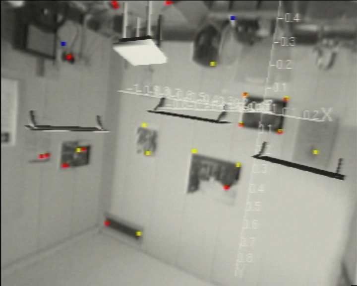
8
system start-up with zero uncertainty. It is now these features which define the world coordinate frame
for SLAM. On the first tracking frame, the camera is held in a certain approximately known location
relative to the target for tracking to start. In the state vector the initial camera position is given an initial
level of uncertainty corresponding to a few degrees and centimeters. This allows tracking to ‘lock on’
very robustly in the first frame just by starting the standard tracking cycle.
D. Motion Modeling and Prediction
After start-up, the state vector is updated in two alternating ways: 1) the prediction step, when the
camera moves in the ‘blind’ interval between image capture, and 2) the update step, after measurements
have been achieved of features. In this section we consider prediction.
Constructing a motion model for an agile camera which is carried by an unknown person, robot or
other moving body may at first glance seem to be fundamentally different to modeling the motion of a
wheeled robot moving on a plane: the key difference is that in the robot case one is in possession of the
control inputs driving the motion, such as ‘move forward 1m with steering angle 5◦ ’, whereas we do not
have such prior information about the agile camera’s movements. However, it is important to remember
that both cases are just points on the continuum of types of model for representing physical systems.
Every model must stop at some level of detail and a probabilistic assumption made about the discrepancy
between this model and reality: this is what is referred to as process uncertainty (or noise). In the case of
a wheeled robot, this uncertainty term takes account of factors such as potential wheel slippage, surface
irregularities and other predominantly unsystematic effects which have not been explicitly modeled. In
the case of an agile camera, it takes account of the unknown dynamics and intentions of the human or
robot carrier, but these too can be probabilistically modeled.
We currently use a ‘constant velocity, constant angular velocity model’. This means not that we assume
that the camera moves at a constant velocity over all time, but that our statistical model of its motion
in a time step is that on average we expect undetermined accelerations occur with a Gaussian profile.
The model is visualized in Figure 2(b). The implication of this model is that we are imposing a certain
smoothness on the camera motion expected: very large accelerations are relatively unlikely. This model
is subtly effective and gives the whole system important robustness even when visual measurements are
sparse.
We assume that in each time step, unknown acceleration aW and angular acceleration αW processes of
zero mean and Gaussian distribution cause an impulse of velocity and angular velocity:
µ W ¶ µ W 
V a ∆t
n= = . (3)
ΩR αR ∆t
Depending on the circumstances, VW and ΩR may be coupled together (for example, by assuming that
a single force impulse is applied to the rigid shape of the body carrying the camera at every time step,
producing correlated changes in its linear and angular velocity). Currently, however, we assume that the
covariance matrix of the noise vector n is diagonal, representing uncorrelated noise in all linear and
rotational components. The state update produced is:
W W
rnew r + (vW + VW )∆t
qW R qW R × q((ω R + ΩR )∆t)
fv = new
=
vnew vW + VW
W
.
(4)
R
ωnew ω R + ΩR
Here the notation q((ω R + ΩR )∆t) denotes the quaternion trivially defined by the angle-axis rotation
vector (ω R + ΩR )∆t.
In the EKF, the new state estimate fv (xv , u) must be accompanied by the increase in state uncertainty
(process noise covariance) Qv for the camera after this motion. We find Qv via the Jacobian calculation:
∂fv ∂fv >
Qv = Pn , (5)
∂n ∂n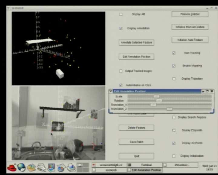
9
y R (up)
x R (left)
Camera Frame R
yW zR (forward)
xW r hL
zW y
World Frame W
(a) (b)
Fig. 3. (a) Frames and vectors in camera and feature geometry. (b) Active search for features in the raw images from the wide-angle
camera. Ellipses show the feature search regions derived from the uncertainty in the relative positions of camera and features and only these
regions are searched.
where Pn is the covariance of noise vector n. EKF implementation also requires calculation of the Jacobian
∂fv
∂xv
. These Jacobian calculations are complicated but a tractable matter of differentiation; we do not present
the results here.
The rate of growth of uncertainty in this motion model is determined by the size of Pn , and setting
these parameters to small or large values defines the smoothness of the motion we expect. With small
Pn , we expect a very smooth motion with small accelerations, and would be well placed to track motions
of this type but unable to cope with sudden rapid movements. High Pn means that the uncertainty in
the system increases significantly at each time step, and while this gives the ability to cope with rapid
accelerations the very large uncertainty means that a lot of good measurements must be made at each
time step to constrain estimates.
E. Active Feature Measurement and Map Update
In this section we consider the process of measuring a feature already in the SLAM map (we will
discuss initialization in the next section).
A key part of our approach is to predict the image position of each feature before deciding which to
measure. Feature matching itself is carried out using a straightforward normalized cross-correlation search
for the template patch projected into the current camera estimate using the method of Section III-B and
the image data — the template is scanned over the image and tested for a match at each location until a
peak is found. This searching for a match is computationally expensive; prediction is an active approach,
narrowing search to maximize efficiency.
First, using the estimates we have xv of camera position and yi of feature position, the position of a
point feature relative to the camera is expected to be:
hR
L = R
RW
(yiW − rW ) . (6)
With a perspective camera, the position (u, v) at which the feature would be expected to be found in
the image is found using the standard pinhole model:
µ ¶ u − f k
hR
Lx
u 0 u hR
hi = = Lz
hR , (7)
v v0 − f kv hRLy
Lz
where f ku , f kv , u0 and v0 are the standard camera calibration parameters.
In the current work, however, we are using wide-angle cameras with fields of view of nearly 100◦ ,
since showing in [6] that the accuracy of SLAM is significantly improved by trading per-pixel angular
resolution for increased field of view — camera and map estimates are much better constrained when
features at very different viewing angles can be simultaneously observed. The imaging characteristics
of such cameras are not well approximated as perspective — as Figure 3(b) shows, its images show
significant non-perspective distortion (straight lines in the 3D world do not project to straight lines in the
image). Nevertheless we perform feature matching on these raw images rather than undistorting them first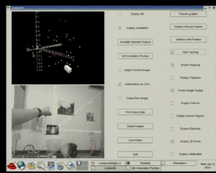
10

(note that the images later must be transformed to a perspective projection for display in order to use
them for augmented reality, since OpenGL only supports perspective camera models).
   We therefore warp the perspective-projected coordinates u = (u, v) with a radial distortion to obtain the
final predicted image position ud = (ud , vd ): The following radial distortion model was chosen because
to a good approximation it is invertible [44]:
                                                         u − u0
                                       ud − u0 = √                                                       (8)
                                                        1 + 2K1 r2
                                                         v − v0
                                       vd − v0 = √                 ,                                     (9)
                                                        1 + 2K1 r2
where                                      p
                                      r = (u − u0 )2 + (v − v0 )2 .                                     (10)
Typical values from a calibration of the camera used in Section IV, calibrated using standard software
and a calibration grid, were f ku = f kv = 195 pixels, (u0 , v0 ) = (162, 125), K1 = 6 × 10⁻⁶ for capture at
320 × 240 resolution.
   The Jacobians of this two-step projection function with respect to camera and feature positions are also
computed (this is a straightforward matter of differentiation easily performed on paper or in software).
These allow calculation of the uncertainty in the prediction of the feature image location, represented by
the symmetric 2 × 2 innovation covariance matrix Si :
                 ∂udi     ∂udi > ∂udi      ∂udi > ∂udi      ∂udi > ∂udi      ∂udi >
            Si =      Pxx       +     Pxyi       +     Py x       +     Py y        +R .               (11)
                 ∂xv      ∂xv     ∂xv      ∂yi     ∂yi i ∂xv        ∂yi i i ∂yi
The constant noise covariance R of measurements is taken to be diagonal with magnitude determined by
image resolution.
   Knowledge of Si is what permits a fully active approach to image search; Si represents the shape of a
2D Gaussian PDF over image coordinates and choosing a number of standard deviations (gating, normally
at 3σ) defines an elliptical search window within which the feature should lie with high probability. In
our system, correlation searches always occur within gated search regions, maximizing efficiency and
minimizing the chance of mismatches. See Figure 3(b).
   Si has a further role in active search; it is a measure of the information content expected of a
measurement. Feature searches with high Si (where the result is difficult to predict) will provide more
information [45] about estimates of camera and feature positions. In Davison and Murray’s work on vision-
based SLAM for a robot with steerable cameras [27] this led directly to active control of the viewing
direction towards profitable measurements; here we cannot control the camera movement, but in the case
that many candidate measurements are available we select those with high innovation covariance, limiting
the maximum number of feature searches per frame to the ten or twelve most informative. Choosing
measurements like this aims to squash the uncertainty in the system along the longest axis available, and
helps ensures that no particular component of uncertainty in the estimated state gets out of hand.
   The obvious points of comparison for our active search technique are very fast bottom-up feature
detection algorithms, which treat an image indiscriminately but can extract all of the features in it in a
few milliseconds. With active search, we will always be able to reduce the amount of image processing
work, but at the potentially significant cost of extra calculations to work out where to search [45]. We do
not claim that active search is sensible if the camera were to become lost — a different process would
be needed to re-localize in the presence of very high uncertainty.

F. Feature Initialization
   With our monocular camera, the feature measurement model cannot be directly inverted to give the
position of a new feature given an image measurement and the camera position since the feature depth is
unknown. Estimating the depth of a feature will require camera motion and several measurements from
different viewpoints. However, we avoid the approach of tracking the new feature in the image for several
11
0.000s 0.033s 0.066s 0.100s 0.133s
Fig. 4. A close-up view of image search in successive frames during feature initialization. In the first frame a candidate feature image patch
is identified within a search region. A 3D ray along which the feature must lie is added to the SLAM map, and this ray is projected into
subsequent images. A distribution of depth hypotheses from 0.5m to 5m translates via the uncertainty in the new camera position relative
to the ray into a set of ellipses which are all searched to produce likelihoods for Bayesian re-weighting of the depth distribution. A small
number of time-steps is normally sufficient to reduce depth uncertainly sufficiently to approximate as Gaussian and enable the feature to be
converted to a fully-initialized point representation.
3.5
3
Probability Density
2.5
2
1.5
1
0.5
0
0.5 1 1.5 2 2.5 3 3.5 4 4.5
Depth (m)
Fig. 5. Frame-by-frame evolution of the probability density over feature depth represented by a particle set. 100 equally-weighted particles
are initially spread evenly along the range 0.5m to 5.0m; with each subsequent image measurement the distribution becomes more closely
Gaussian.
frames without attempting to estimate its 3D location at all, then performing a mini-batch estimation step
to initialize its depth from multiple view triangulation. This would violate our top-down methodology
and waste available information: 2D tracking is potentially very difficult when the camera is potentially
moving fast. Additionally, we will commonly need to initialize features very quickly because a camera
with a narrow field of view may soon pass them by.
The method we use instead after the identification and first measurement of a new feature is to initialize
a 3D line into the map along which the feature must lie. This is a semi-infinite line, starting at the estimated
camera position and heading to infinity along the feature viewing direction, and like otherµmap members 
rWi
has Gaussian uncertainty in its parameters. Its representation in the SLAM map is: ypi = where
ĥW
i
ri is the position of its one end and ĥWi is a unit vector describing its direction.
All possible 3D locations of the feature point lie somewhere along this line, but we are left with one
degree of freedom of its position undetermined — its depth, or distance along the line from the endpoint.
A set of discrete depth hypotheses is uniformly distributed along this line, which can be thought of as
a one-dimensional probability density over depth represented by a 1D particle distribution or histogram.
Now we make the approximation that over the next few time-steps as this new feature is re-observed,
measurements of its image location provide information only about this depth coordinate, and that their
effect on the parameters of the line is negligible. This is a good approximation because the amount of
uncertainty in depth is very large compared with the uncertainty in the line’s direction. While the feature
is represented in this way with a line and set of depth hypotheses we refer to it as partially initialized.
Once we have obtained a good depth estimate in the form of a peaked depth PDF, we convert the feature
to ‘fully initialized’ with a standard 3D Gaussian representation.
At each subsequent time step, the hypotheses are all tested by projecting them into the image, where
each is instantiated as an elliptical search region. The size and shape of each ellipse is determined by the12
uncertain parameters of the line: each discrete hypothesis at depth λ has 3D world location yλi = rW W
i +λĥi
. This location is projected into the image via the standard measurement function and relevant Jacobians
of Section III-E to obtain the search ellipse for each depth. Note that in the case of a non-perspective
camera (such as the wide-angle cameras we normally use), the centers of the ellipses will not lie along
a straight line, but a curve. This does not present a problem as we treat each hypothesis separately.
We use an efficient algorithm to make correlation searches for the same feature template over this
set of ellipses, which will typically be significantly overlapping (the algorithm builds a look-up table of
correlation scores so that image processing work is not repeated for the overlapping regions). Feature
matching within each ellipse produces a likelihood for each, and their probabilities are re-weighted via
Bayes’ rule: the likelihood score is simply the probability indicated by the 2D Gaussian PDF in image
space implied by the elliptical search region. Note that in the case of many small ellipses with relatively
small overlaps (true when the camera localization estimate is very good), we get much more resolving
power between different depth hypotheses than when larger, significantly overlapping ellipses are observed,
and this affects the speed at which the depth distribution will collapse to a peak.
Figure 4 illustrates the progress of the search over several frames, and Figure 5 shows a typical
evolution of the distribution over time, from uniform prior to sharp peak. When the ratio of the standard
deviation of depth to depth estimate drops below a threshold (currently 0.3), the distribution is safely
approximated as Gaussian and the feature initialized as a point into the map. Features which have
just crossed this threshold typically retain large depth uncertainty (see Figure 1(a) which shows several
uncertainty ellipsoids elongated along the approximate camera viewing direction), but this shrinks quickly
as the camera moves and further standard measurements are obtained.
The important factor of this initialization is the shape of the search regions generated by the overlapping
ellipses. A depth prior has removed the need to search along the entire epipolar line, and improved the
robustness and speed of initialization. In real-time implementation, the speed of collapse of the particle
distribution is aided (and correlation search work saved) by deterministic pruning of the weakest hypotheses
at each step, and a during typical motions around 2–4 frames is sufficient. It should be noted that most
of experiments we have carried out have involved mostly sideways camera motions and this initialization
approach would perform more poorly with motions along the optic axis where little parallax is measured.
Since the initialization algorithm of this section was first published in [5], some interesting developments
to the essential idea have been published. In particular, Solà et al. [46] have presented an algorithm which
represents the uncertainty in a just-initialized feature by a set of overlapping 3D Gaussian distributions
spaced along the 3D initialization line. Appealing aspects of this approach are firstly the distribution of
the Gaussians, which is uniform in inverse depth rather than uniform in depth as in our technique —
this appears to be a more efficient use of multiple samples. Also their technique allows measurements of
new features immediately to have an effect on refining the camera localization estimate, improving on our
need to wait until the feature is ‘fully-initialized’. Most recently, Montiel et al. [47] have shown that a
re-parametrization in terms of inverse depth permits even more straightforward and efficient initialization
within the standard EKF framework, in an approach similar to that used by Eade and Drummond [42] in
a new FastSLAM-based monocular SLAM system.
G. Map Management
An important part of the overall algorithm is sensible management of the number of features in the map,
and on-the-fly decisions need to be made about when new features should be identified and initialized, as
well as when it might be necessary to delete a feature. Our map-maintenance criterion aims to keep the
number of reliable features visible from any camera location close to a pre-determined value determined
by the specifics of the measurement process, the required localization accuracy and the computing power
available: we have found that with a wide-angle camera a number in the region of 12 gives accurate
localization without over-burdening the processor. An important part of our future work plan is to put
heuristics such as this on a firm theoretical footing using methods from information theory as discussed
in [45].13
state
estimate update
xp
n π R
update predict search measurement
normal
Camera 0 z
image
patch predict
t
appearance
normal
x
Camera 1 estimate
y
(a) (b)
Fig. 6. (a) Geometry of a camera in two positions observing a surface with normal n. (b) Processing cycle for estimating the 3D orientation
of planar feature surfaces.
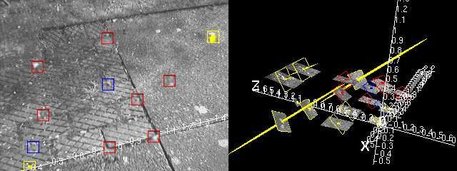
Fig. 7. Results from real-time feature patch orientation estimation, for an outdoor scene containing one dominant plane and an indoor
scene containing several. These views are captured from the system running in real-time after several seconds of motion, and show the initial
hypothesized orientations with wire-frames and the current estimates with textured patches.
Feature ‘visibility’ (more accurately, predicted measurability) is calculated based on the relative position
of the camera and feature, and the saved position of the camera from which the feature was initialized.
The feature must be predicted to lie within the image, but also the camera must not have translated too
far from its initialization viewpoint of the feature or we would expect correlation to fail (note that we can
cope with a full range of rotation). Features are added to the map only if the number visible in the area
the camera is passing through is less than this threshold — it is undesirable to increase the number of
features and add to the computational complexity of filtering without good reason. Features are detected
by running the image interest operator of Shi and Tomasi to locate the best candidate within a box of
limited size (around 80 × 60 pixels) placed within the image. The position of the search box is currently
chosen randomly, with the constraints only that it should not overlap with any existing features and that
based on the current estimates of camera velocity and angular velocity any detected features are not
expected to disappear from the field of view immediately.
A feature is deleted from the map if, after a predetermined number of detection and matching attempts
when the feature should be visible, more than a fixed proportion (in our work 50%) are failures. This
criterion prunes features which are ‘bad’ for a number of possible reasons: they are not true 3D points
(lying at occlusion boundaries such as T-junctions), lie on moving objects, are caused by specular highlights
on a curved surface, or important are just often occluded.
Over a period of time, a ‘natural selection’ of features takes place through these map management
criteria which leads to a map of stable, static, widely-observable point features. Clutter in the scene
can be dealt with even if it sometimes occludes these landmarks, since attempted measurements of the
occluded landmarks simply fail, and do not lead to a filter update. Problems only arise if mismatches
occur due to a similarity in appearance between clutter and landmarks, and this can potentially lead to
catastrophic failure. Note however that mismatches of any kind are extremely rare during periods of good
tracking since the large feature templates give a high degree of uniqueness and the active search method
means that matching is usually only attempted within very small image regions (typically 15–20 pixels
across).14
H. Feature Orientation Estimation
In Section III-B we described how visual patch features extracted from the image stream are inserted
into the map as oriented, locally-planar surfaces, but explained that the orientations of these surfaces are
initially just postulated, this proving sufficient for calculating the change of appearance of the features
over reasonable viewpoint changes. This is the approach used in the applications presented in Sections IV
and V.
In this section we show as in [7] that it is possible to go further, and use visual measurement within
real-time SLAM to actually improve the arbitrarily assigned orientation for each feature and recover real
information about local surface normals at the feature locations. This improves the range of measurability
of each feature, but also takes us a step further towards a possible future goal of recovering detailed 3D
surface maps in real-time rather than sets of sparse landmarks.
Our approach shares some of the ideas of Jin et al. [48] who described a sequential (but not real-
time) algorithm they described as ‘direct structure from motion’ which estimated feature positions and
orientations. Their concept of their method as ‘direct’ in globally tying together feature tracking and
geometrical estimation is the same as the principles of probabilistic SLAM and active search used over
several years in our work [5], [27]. They achieve impressive patch orientation estimates as a camera moves
around a highly textured object.
Since we assume that a feature corresponds to a locally planar region in 3D space, as the camera
moves its image appearance will be transformed by changes in viewpoint by warping the initial template
captured for the feature. The exact nature of the warp will depend on the initial and current positions
of the camera, the 3D position of the center of the feature, and the orientation of its local surface. The
SLAM system provides a running estimate of camera pose and 3D feature positions. We now additionally
maintain estimates of the initial camera position and the local surface orientation for each point. This
allows a prediction of the feature’s warped appearance from the current viewpoint. In the image, we then
make a measurement of the current warp, and the difference between the prediction and measurement is
used to update the surface orientation estimate.
Figure 6(a) shows the geometry of a camera in two positions viewing an oriented planar patch. The
warping which relates the appearance of the patch in one view to the other is described by the homography:
H = CR[nT xp I − tnT ]C−1 , (12)
where C is the camera’s calibration matrix, describing perspective projection or a local approximate
perspective projection in our images with radial distortion, R and t describe the camera motion, n is
the surface normal and xp is the image projection of the center of the patch (I is the 3 × 3 identity
matrix).
It is assumed that this prediction of appearance is sufficient for the current image position of the
feature to be found using a standard exhaustive correlation search over the two image coordinates within
an elliptical uncertainty region derived from the SLAM filter. The next step is to measure the change
in warp between the predicted template and the current image. Rather than widening the exhaustive
search to include all of the degrees of freedom of potential warps, having locked down the template’s
2D image position we proceed with a more efficient probabilistic inverse-compositional gradient-descent
image alignment step [49], [50] to search through the additional parameters, on the assumption that the
change in warp will be small and that this search will find the globally best fit.
Figure 6(b) displays graphically the processing steps in feature orientation estimation. When a new
feature is added to the map, we initialize an estimate of its surface normal which is parallel to the
current viewing direction, but with large uncertainty. We currently make the simplifying approximation
that estimates of feature normals are only weakly correlated to those of camera and feature positions.
Normal estimates are therefore not stored in the main SLAM state vector, but maintained in a separate
two-parameter EKF for each feature.
Figure 7 shows results from the patch orientation algorithm in two different scenes: an outdoor scene
which contains one dominant plane and an indoor scene where several boxes present planes at different15
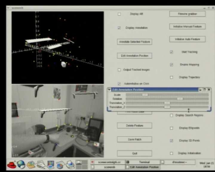
Hand-held camera Camera and scene Initializing features Active search ellipses
External view of cam- Object insertion GUI:
Inserting and adjusting Requesting a small table
era location estimate and pointing to desired shelf
shelf
mapped features location
Scene with four inserted Tracking through extreme Tracking through signifi-
Close-up of shelves
objects rotation cant occlusion
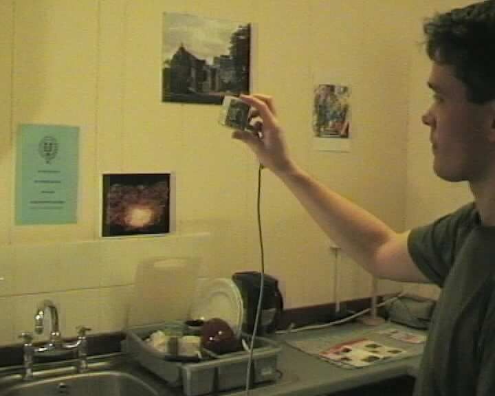
Fig. 8. Frames from a demonstration of real-time augmented reality using MonoSLAM, all acquired directly from the system running in
real-time at 30Hz. Virtual furniture is inserted into the images of the indoor scene observed by a hand-held camera. By clicking on features
from the SLAM map displayed with real-time graphics, 3D planes are defined to which the virtual objects are attached. These objects then
stay clamped to the scene in the image view as the camera continues to move. We show how the tracking is robust to fast camera motion,
extreme rotation and significant occlusion.
orientations. Over a period of several seconds of tracking in both cases, the orientations of most of mapped
feature patches are recovered well.
In general terms, it is clear that orientation estimation only works well with patches which are large
and have significant interesting texture over their area, because in this case the image alignment operation
can accurately estimate the warping. This is a limitation as far as estimating an accurate normal vector at
every feature location, since many features have quite simple texture patterns like a black on white corner,
where full warp estimation is badly constrained. The scenes in our examples are somewhat artificial in
that both contain large planar areas with significant flat texture.
However, it should be remembered that the current motivation for estimating feature orientations in our
work is to improve the range of camera motion over which each long-term landmark will be measurable.
Those features for which it is difficult to get an accurate normal estimate are exactly those where doing
so is less important in the first place, since they exhibit a natural degree of viewpoint-invariance in their
appearance. It does not matter if the normal estimate for these features is incorrect because it will still be
possible to match them. We see this work on estimating feature surface orientation as part of a general
direction towards recovering more complete scene geometry from a camera moving in real-time.
IV. R ESULTS : I NTERACTIVE AUGMENTED R EALITY
Before presenting a robotics application of MonoSLAM in Section V, in this section we give results
from the use of our algorithm in an augmented reality scenario, as virtual objects are inserted interactivelyYou can also read