Local acoustic habitat relative to hearing sensitivities in beluga whales (Delphinapterus leucas)
←
→
Page content transcription
If your browser does not render page correctly, please read the page content below
JOURNAL OF ECOACOUSTICS
                                                                                                                www.veruscript.com/jea

Local acoustic habitat relative to hearing sensitivities
in beluga whales (Delphinapterus leucas)
Original paper                                     T. Aran Mooney1*, Manuel Castellote2,3, Ian T. Jones1, Lori Quakenbush4,
                                                   Roderick Hobbs3, Eric Gaglione5, Caroline Goertz6
Article history:
                                                   1
                                                    Biology Department, Woods Hole Oceanographic Institution, Woods Hole, MA 02543, USA
Received: 1 December 2017                          2
                                                     Joint Institute for the Study of the Atmosphere and Ocean ( JISAO), University of Washington,
Accepted: 30 April 2018                            3737 Brooklyn Avenue NE, Seattle, WA 98105, USA
Published: 20 June 2018                            3
                                                    Marine Mammal Laboratory, Alaska Fisheries Science Center, National Marine Fisheries Service,
                                                   Seattle, WA 98115, USA
                                                   4
                                                     Alaska Department of Fish and Game, 1300 College Road, Fairbanks, AK 99701, USA
                                                   5
                                                    Georgia Aquarium, 225 Baker St NW, Atlanta, GA 30313, USA
*Correspondence:                                   6
                                                     Alaska SeaLife Center, 301 Railway Ave, Seward, AK 99664, USA
TAM: amooney@whoi.edu

                                                   Abstract
Peer review:
Double blind                                       Background noise can have a substantial effect on communication signals,
                                                   however far less is known about how natural soundscapes may influence
Copyright:                                         hearing sensitivity. Here we compare the audiograms of 26 wild beluga
© 2018 Mooney et al. This is an open               whales measured in their natural environment to a series of ecoacoustic
access article distributed under the Creative      measurements within a primary portion of their Bristol Bay summer habitat,
Commons Attribution License (CC-BY 4.0),           the Nushagak Estuary in Bristol Bay, AK, USA. Environmental acoustic
which permits unrestricted use, distribution,      measurements were made during 2012 and 2016 using two different
and reproduction in any medium, provided           methods: a moored recorder and drifter buoys. Environmental noise curves
the original work is properly cited and its        varied substantially. Drifter recordings from the middle of Nushgak Estuary
authors credited.                                  had the highest spectrum levels during ebb tides with acoustic energy from
                                                   sediment transport extending well into higher frequencies (ca. 60 kHz),
Keywords:
                                                   likely due to rapidly moving tidal flow and shifting sediment in that location.
noise; soundscape; cetacean; odontocete;
                                                   Drifter recordings near the estuary mouth and shallow tidal flats were lower
arctic
                                                   amplitude. Noise levels generally varied during drifts (in one case up to ca.
Citation:                                          6 dB) reflecting acoustic cues available to the local belugas. The moored
Mooney T. A., Castellote M., Jones I. T.,          recorder showed a substantially different spectral profile, especially at lower
Quakenbush L., Hobbs R., Gaglione E., and          frequencies, perhaps due to its attachment to a pier piling and subsequent
Goertz C. (2018). Local acoustic habitat           pier noise. Hearing sensitivity varied by individual and thresholds often fell
relative to hearing sensitivities in beluga        above 1/3 octave-band noise levels, but not overall noise spectral density.
whales (Delphinapterus leucas). Journal of         Audiograms of the most sensitive animals closely paralleled the lowest
Ecoacoustics. 2: #QZD9Z5.                          ambient noise power spectral density curves, suggesting that an animal’s
https://doi.org/10.22261/JEA.QZD9Z5                auditory dynamic range may extend to include its habitat’s quietest condi-
                                                   tions. These data suggest a cautious approach is necessary when estimating
                                                   the sound-sensitivity of odontocetes found in quiet environments as they
                                                   may have sensitive auditory abilities that allow for hearing within the lowest
                                                   noise-level conditions. Further, lower level ambient noise conditions could
                                                   provide a conservative estimate of the maximal sensitivity of some cetacean
                                                   populations within specific environments.

                                                   Introduction

                                                   Understanding a population’s habitat is vital to proper conservation and
                                                   management, therefore it is important to address natural variability and
                                                   how microhabitats may influence a taxon in different ways. Acoustics of
                                                   the ocean in general has long been investigated but more recently
                                                   soundscapes (encompassing all sounds within an area) of specific habitats
                                                   or larger ecosystems have received greater emphasis (e.g., Haver et al.,

J. Ecoacoust. | 2018 | 2: #QZD9Z5 | https://doi.org/10.22261/JEA.QZD9Z5                                                                              1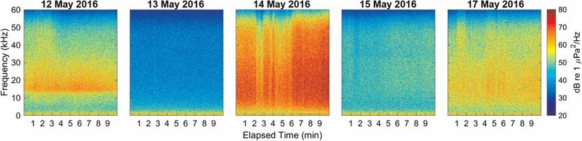
Mooney et al. | Low noise enables sensitive beluga hearing                       https://www.veruscript.com/a/JEA.QZD9Z5/

2017; Menze et al., 2017; Reeves et al., 2017; Stafford et al., 2018). Thus in many areas, from coral reefs to the
Arctic, we are still seeking to describe the variability in the acoustic environment found within a habitat.
   Animals will use or be influenced by the soundscape they experience. Acoustic cues within an environment
can provide vital information for detecting predators, localizing prey, navigating to safe habitat or shaping the
communication among conspecifics. High levels of background noise, however, can limit the detection or
recognition of important signals (Au, 1993; Erbe and Farmer, 1998; Clark et al., 2009). Elevated environmental
noise levels might be critical in cases where these cues or signals are of low amplitude. And indeed, we find
many vital signals to be relatively quiet (Tyack and Clark, 2000; Li et al., 2008; Holt et al., 2009); for them to
be properly received and distinguished requires both sensitive hearing and relatively low background noise levels.
   Among aquatic animals, odontocetes have relatively sensitive hearing (Webster et al., 1992; Nachtigall et al.,
2000; Mooney et al., 2012), however, as for many taxa, this sensitivity can vary within a species or population
where some animals (often younger ones) have sensitive hearing and others have elevated, impaired thresholds
(Houser and Finneran, 2006b). Unfortunately, we do not have estimates for hearing variability in most cetacean
populations, nor do we know their auditory thresholds relative to their natural acoustic habitat. Quantifying the
audiograms of animals simultaneously with their acoustic habitat may provide insight into whether hearing is
adapted to particular conditions of their environment, and how hearing is influenced by the natural variability in
the ambient noise of that habitat.
   Animal hearing and its relationship to the natural acoustic environment provides the context needed to under-
stand the potential negative effects of anthropogenic noise on acoustic habitat. Human-produced noise has
rapidly increased in the ocean in recent years (McDonald et al., 2006; Hildebrand, 2009; Gedamke, 2016) from
sources such as commercial shipping, underwater construction, resource extraction, scientific exploration, and
military activities. This noise can have diverse and potentially serious effects on marine mammals (National
Academy of Sciences, 2003, 2005). Most of our understanding focuses on the impacts of intense sources and
high received levels addressing affects such as avoidance responses and temporary hearing loss (Mooney et al.,
2009; Tougaard et al., 2009; Tyack et al., 2011). If hearing is sensitive, soundscapes are quiet, and vital cues are
of low intensity, even small increases in background noise may have detrimental effects (e.g., not detecting or
discriminating sounds). Given the pervasiveness of vessel traffic and many other human noise sources, measure-
ments of “quiet”, natural habitats are becoming harder to record. Yet to adequately assess the influence of
increasing noise it is critical that we compare hearing information to soundscape data, and ideally soundscape
data without human-noise contributors.
   In an effort to address habitat specific sound-sensitivity we need to acquire hearing and soundscape measure-
ments in the same locations and general context. In this study, we measured the hearing of 26 wild beluga whales
(Delphinapterus leucas) and the acoustic environment of a component of their spring-summer habitat in Bristol
Bay, Alaska using two different passive acoustic methods. Belugas are highly dependent on hearing and under-
water sound as their primary sensory modality for vital biological activities including foraging, communication
with conspecifics and navigation (Au et al., 2000; Mooney et al., 2008; Castellote et al., 2014). Beluga whales
have been identified as Arctic ecosystem sentinels because they are broadly dispersed, high trophic-level feeders
and are an important cultural and nutritional species for native Arctic peoples (Moore and Huntington, 2008).
Adjacent to the Togiak National Wildlife Refuge, Bristol Bay is a relatively well-protected habitat. The beluga
population, estimated at 3,000 animals, is considered healthy (Allen and Angliss, 2014). For several months in
the summer, Bristol Bay is home to the largest sockeye salmon (Onchorynchus nerka) run and fishery in the
world. Yet, most of the year, beluga habitat can be considered minimally disturbed and thus a representative
soundscape of a natural estuary ecosystem. We compared our audiograms and background noise measurements
to understand hearing sensitivity with respect to variability in a soundscape habitat.

Methods

Study overview
This study builds from a prior, initial hearing study of a wild population beluga whales. Following these
methods (Castellote et al., 2014; Mooney et al., 2016) we increased the sample size of audiograms to 26 belugas
(Mooney et al., 2018). Hearing was measured in a capture-release setting in Bristol Bay, AK, USA. These data
were collected during three ca. 14-day seasons in August-September 2012, September 2014, and May 2016.
Ambient soundscape measurements were made during the 2012 and 2016 study periods. The hearing assess-
ments were part of a beluga whale health assessment program coordinated by the National Marine Fisheries
Service and the Alaska SeaLife Center following capture and holding procedures similar to those used in the
J. Ecoacoust. | 2018 | 2: #QZD9Z5 | https://doi.org/10.22261/JEA.QZD9Z5                                                 2
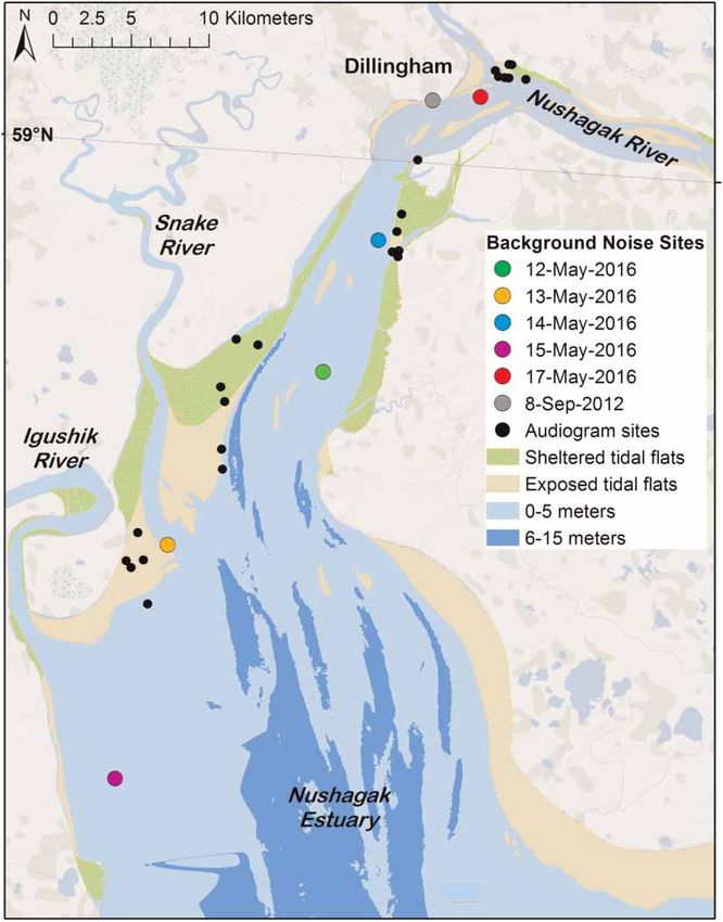
Mooney et al. | Low noise enables sensitive beluga hearing                         https://www.veruscript.com/a/JEA.QZD9Z5/

Figure 1. Map of the Nushagak Estuary of Bristol Bay, Alaska, USA with the audiogram measurement sites (i.e.,
capture sites) indicated by the black dots and locations of ambient soundscape measurements indicated by the
colored dots.
Audiograms and soundscape measurements were conducted in August-September 2012 and May 2016.

2000s (Citta et al., 2016). Additional health and biological assessments were concurrently made on each individ-
ual animal during ca. 2 h holding period (Norman et al., 2012), after which the animals were released. The
study was conducted under National Marine Fisheries Service marine mammal research permit #14245 and
approved by WHOI and NOAA Fisheries, Alaska Fisheries Science Center’s Institutional Animal Care and Use
Committees. Capture-and-release events occurred in the Nushagak Estuary (Figure 1), one of the two arms of
the Bristol Bay Estuary Ecosystem used by Bristol Bay beluga whales.

Soundscape measurements
Acoustic recordings were made using two methods. In 2012, a programmable DSG-Ocean acoustic data-logger
(Loggerhead Instruments, Sarasota, FL, USA) was attached to a pile-pole at an unused cannery pier in Dillingham,
AK, during low tide 1 m from the seafloor and facing open-water. The DSG had a HTI-96-Min hydrophone (High
Tech Inc. Gulfport, MS, USA) with -185.8 dB re 1 V/mPa receiving sensitivity, 20 dB gain, and frequency response
variability of ±1 dB from 2 Hz to 40 kHz. The acoustic data-logger was set to record continuously at 80 kHz sample
rate and was deployed for 4 days while the beluga captures took place. This site was centrally located amongst the
capture-release locations. Recordings for analysis were selected based on the sea state and the tide cycle. During the
selection, recordings were manually scanned to check quality, confirm that the instrument was below the surface and
check whether identifiable anthropogenic noise sources were absent. A total of 16 min of recordings were selected
across 8 and 9 September 2012, corresponding to periods of sea state 0–1 in flooding (ca. 5 min), high/slack (ca.
5 min), and ebbing (ca. 5 min) tidal cycles. The median spectral curve was calculated in 1 s integration bins for
every second of the selected recording periods across the full band of 2 Hz–40 kHz.
   To gather more spatial coverage, in 2016, we used a custom drifter buoy instrumented with a DMON recorder
(serial number 17a, Woods Hole Oceanographic Institution) configured with a low-noise preamplifier (20 dB
J. Ecoacoust. | 2018 | 2: #QZD9Z5 | https://doi.org/10.22261/JEA.QZD9Z5                                                   3
Mooney et al. | Low noise enables sensitive beluga hearing                                        https://www.veruscript.com/a/JEA.QZD9Z5/

gain), 13.2 dB user programmable gain, a 16-bit analog-to-digital converter, and 32 GB of flash memory. The
DMON was programmed to record from its mid-frequency hydrophone (Navy type II ceramics, with −200 dB re.
1 V μPa receiving sensitivity), sampling at 120 kHz with a 6-pole Sallen-Key antialiasing low-pass filter at 60 kHz
and high pass filter at 100 Hz and a −172 dB sensitivity ±3 dB within that 0.1–60 kHz range.
   The drifter buoy consisted of a spherical surface float with the DMON suspended 1.5 m below the surface on
a weighted line and deployed from a boat. After deployment, the boat moved ∼1,000 m away from the buoy,
shut off its motor and drifted for 15–20 min, and then the boat picked up the drifting buoy. Recordings were
edited using Adobe Audition CS5.5 to remove the initial and final periods of the recording to exclude boat and
motor noise, and recordings were inspected to remove any transient signal or self-noise prior to the analysis.
Total duration of the edited recording files was standardized to 10 min. Samples were collected at 5 locations
across the region where belugas were captured during the health sampling within the Nushagak Estuary
(Figure 1; Table 1). For all samples, sea state was 0–1 with no precipitation and no other boats within visible
(naked-eye) range.
   All sound recordings from 2012 and 2016 were processed with custom written Matlab scripts, or in
SpectraPRO 732 (Sound Technology Corporation) in the case of 2012 power spectral density (PSD) data, to
calculate instantaneous pressure in μPa after accounting for the system gain and hydrophone receiving sensitivity.
To address how sound levels varied between sites, we calculated PSD in dB re 1 mPa2/Hz as well as 1/3 octave
band levels in root mean square sound pressure level (dBrms re 1 mPa). The PSD was calculated from 0.1 to
40 kHz using the Fast Fourier transform (FFT) algorithm with a Hanning window equal to the recorder’s
sampling rate (80,000 point Hanning window for 2012 DSG data, 120,000-point window for 2016 DMON
data), with 50% overlap, providing a frequency resolution of 1 Hz. Sound pressure level (SPL) curves were calcu-
lated in 1/3 and 1/12 octave bands filtered using Butterworth filters with center frequencies from 0.25 to
32 kHz and using the base 10 method. For comparison, SPL noise levels were also calculated in 1/6 octave band
filters (see Supplementary Figure). For each recording location, PSD and SPL were calculated over 1 min integra-
tions and the median value for each frequency bin was found. For 1/3 octave band curves, the variance across
these 1 min time periods was described by the 25th and 75th percentiles.
   To assess how sound levels changed over the 2016 sampling periods, root mean square sound pressure level
was also calculated in 1 s integration bins for every second of the 10-min file across the full band of 100 Hz–
60 kHz, using a 4th order Butterworth filter. With only five locations to compare we used the mean spectral
curve to estimate the average sound pressure levels over time within all sites. This was done at each center
frequency measurement and every 1 s from all 10-min files. To visualize the site variability over time, frequency
and sound level, 10-min spectrograms of the 5 locations were calculated in power spectral density in 1 Hz bins
using Welch’s method with a 120,000-point Hanning window, a 1 s integration time and 50% overlap.

AEP hearing tests
Methods are briefly summarized below; for greater details on the hearing test methods and population level
hearing parameters see: (Castellote et al., 2014; Mooney et al., 2016, 2018). During the hearing tests the whales
were positioned adjacent to a small inflatable boat. Hearing was tested using AEP methods similar to other AEP

Table 1. Location and time of background noise recordings from the moored recorder and drifter buoy.

       Date                   Lat                   Lon                   Time of rec start (local)      Tide status

       9/8–9/2012             59 2.117N             158 28.383W           11:00                          Ebbing, high, flooding

       6/12/2016              58 52.575N            158 34.175W           18:50                          Flooding mid

       6/13/2016              58 46.235N            158 43.768W           20:12                          Flooding mid

       6/14/2016              58 57.257N            158 31.061W           20:42                          Flooding 1st 1/2

       6/15/2016              58 38.032N            158 46.137W           14:38                          Ebbing mid

       6/17/2016              59 2.434N             158 24.835W           16:04                          Ebbing 1st 1/2

J. Ecoacoust. | 2018 | 2: #QZD9Z5 | https://doi.org/10.22261/JEA.QZD9Z5                                                                  4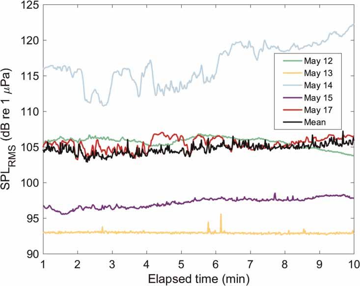
Mooney et al. | Low noise enables sensitive beluga hearing                        https://www.veruscript.com/a/JEA.QZD9Z5/

studies and identical to those described elsewhere (ibid). The AEP equipment was outfitted in a ruggedized case
and the operator sat in the small inflatable boat beside the beluga.
   Hearing was measured using sinusoidally amplitude modulated (SAM) tone-bursts (Nachtigall et al., 2007),
digitally synthesized with a customized LabVIEW (National Instruments, Austin, TX, USA) data acquisition
(DAQ) program and a National Instruments PCMCIA-6062E DAQ card implemented in a semi-ruggedized
Panasonic Toughbook laptop computer. Each SAM tone-burst was 20-ms long, created using a 512 kHz sample
rate and presented at a rate of 20/s. The carrier frequencies were modulated at a rate of 1,000 Hz, with a 100%
modulation depth. The brief SAM tones create some minor sidebands (see Supplementary Material) but these
were substantially lower than the center frequency, minimal at low amplitudes (near thresholds) and were not
expected to impact hearing estimates (Supin and Popov, 2007).
   The test tones were played to the beluga using a “jawphone” transducer located 4 cm from the tip of the lower
jaw on the animal’s medial axis. The jawphone consisted of a Reson 4013 transducer (Slangerup, Denmark)
implanted in a custom silicone suction-cup. The jawphone method was chosen because belugas freely moved their
heads during the experiments; this would have provided varying sound received levels for a free-field transducer.
By always placing the jawphone at one consistent location (i.e., the tip of the lower jaw), it was possible to easily
provide comparable stimuli within a session and between animals despite movement of their heads. The specific
location was used because it has been identified as a region of primary acoustic sensitivity for belugas (Mooney
et al., 2008) and it likely ensonified both ears equally. Prior studies have also shown comparable audiograms
between jawphone and free-field measurements (Finneran and Houser, 2006; Houser and Finneran, 2006a).
   Hearing was tested at multiple frequencies (4–180 kHz) although not all frequencies were tested on all animals
because of the time limitations associated with each capture situation. The stimuli were calibrated each year both
prior to, and immediately after, the experiment. During calibration, the jawphone projector and Reson 4013
receiver were placed in salt water 50 cm apart at 1 m depth. Fifty cm is the approximate distance from jaw tip to
auditory bulla in an adult beluga. The received signals were viewed on an oscilloscope and the peak-to-peak
voltages (Vp-p) were measured. These values were then calculated into sound pressure levels (dBp-p re 1 μPa)
(Au, 1993). This SPLp-p was converted to calculate peak equivalent RMS ( peRMS) by subtracting 15 dB, an
estimate of RMS dB, which was then used to calculate the SPL (Supin et al., 2001; Nachtigall et al., 2008).
   Evoked potential recordings were made using gold EEG electrodes (Grass Technologies, Warwick, RI, USA)
embedded in custom-built silicone suction cups. The active electrode was attached about 3–4 cm behind the
blowhole approximately over the brainstem. The reference (inverting) electrode was attached distal to the active
electrode, on the animal’s back typically near the anterior terminus of the dorsal ridge. A third suction-cup
sensor was also placed dorsally, typically posterior to the dorsal ridge.
   The electrodes were connected to a biological amplifier (CP511, Grass Technologies), which amplified all
responses 10,000-fold and bandpass filtered (300–3,000 Hz). The AEP data were finally imputed into the laptop
and recorded using the same DAQ card and custom program. Responses were sampled at 16 kHz and 30-ms
sweeps beginning coincident with stimulus presentation. Stimuli were presented 500 times for each sound level
and 500 corresponding AEP responses were averaged and stored for later data analyses. Sound levels were decreased
in steps of 5–10 dB until responses (evoked responses and FFT peaks) were no longer visually detectable for two
to three trials. Decibel step size was based on the amplitude of the signal and the animal’s neurological response.
   Audiogram thresholds were calculated offline. Records were initially viewed in the time-domain. A 16-ms
portion of this record, from 5 to 21 ms, was then converted to the frequency domain by calculating a 256-point
FFT. The FFT provided a peak at the 1,000 Hz signal modulation rate. This peak value was used to estimate
the magnitude of the response evoked. These values were then plotted as response intensity against SPL of
the stimulus at a given frequency. A linear regression addressing the data points was then used to find the
hypothetical point where there would be no response and thus the animal’s threshold. Analyses were conducted
using EXCEL, Matlab and MINITAB software.

Results and discussion

Comparisons within the estuary
Soundscape recordings and audiograms were made throughout Nushagak Estuary beluga habitat (Figure 1), and
the acoustic environment in this area showed an important level of variability (Figure 2). The PSD curves for
each of 2016s 5-days sampled with a drifter buoy showed background noise levels were quite variable when
measured at different locations across the bay. Differences among locations were as large as 31.8 dB at 17 kHz
(Figure 2). Three of the 5 measurement locations (12th, 14th and 17th May 2016) showed higher PSD values
J. Ecoacoust. | 2018 | 2: #QZD9Z5 | https://doi.org/10.22261/JEA.QZD9Z5                                                  5
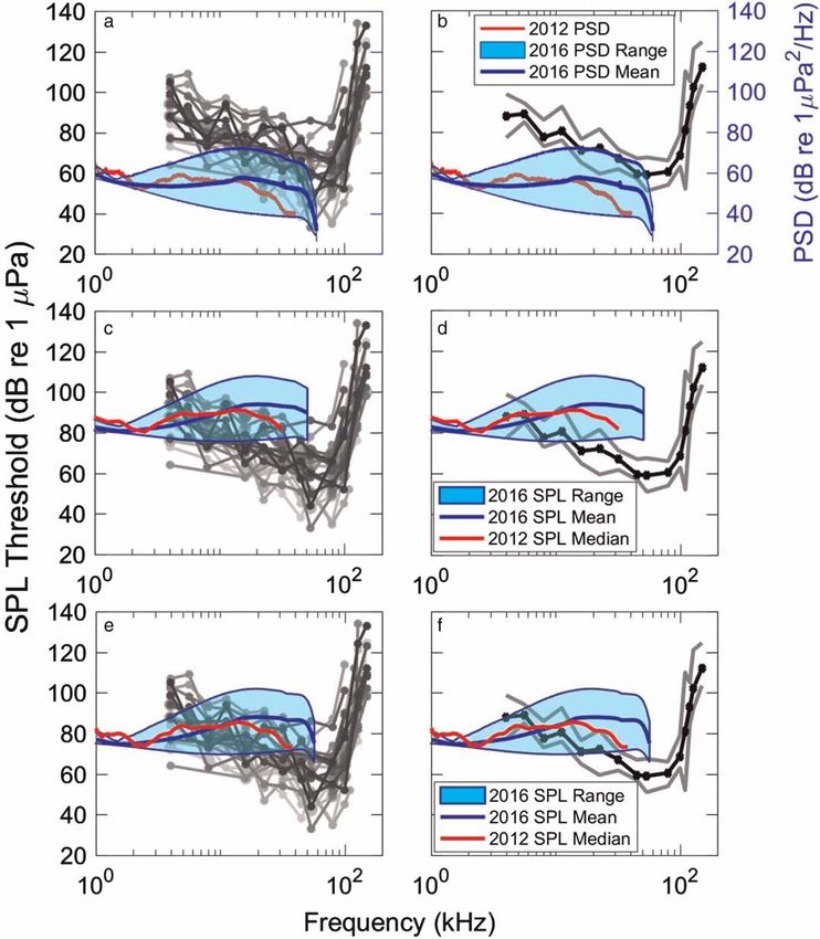
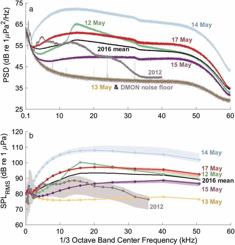
Mooney et al. | Low noise enables sensitive beluga hearing                                   https://www.veruscript.com/a/JEA.QZD9Z5/

Figure 2. Ambient noise levels of beluga habitat measured in the Nushagak Estuary of Bristol Bay.
(a) Ambient soundscape spectra (median power spectral density, 1 min integration) for one 2012 location and five 2016 locations
measured in the Nushagak Estuary of Bristol Bay, AK, USA. The mean of the five 2016 locations is also shown. Note that the DMON
noise floor (dotted curve) overlaps with the 13 May data (yellow curve), indicating that the soundscape recorded on 13 May did not
exceed spectral levels of the recording instrument’s electronic noise floor. (b) Root mean square sound pressure levels calculated in
1/3 octave bands showing the respective median values (1 min integration) for each location ±25–75% ranges.

than the average (Figure 2). These locations were farther north into the Nushagak Estuary, where the river
configuration is narrower and thus currents are stronger than in the lower end of the estuary, near the entrance
to Bristol Bay. Also, these locations were further away from shore, closer to the main river channel where currents
are also expected to be stronger. The elevated noise levels observed at these locations were likely due to sediment
transport noise by current flow (Thorne, 1985; Barton et al., 2010; Bassett et al., 2013). These authors show
how the inter-particle collisions of bedload material (coarse sand and gravel) significantly increase noise levels
often from 4 to 30 kHz. But at times, this sediment noise can extend far into the ultrasonic, near 100 kHz,
depending on grain size and current speed (ibid). This elevated background noise is typical of other tidal
estuaries (e.g., Bassett et al., 2013; Castellote et al., 2016). The spectral curve for 13 May 2016 was at the
electrical noise floor of the recording instrument (DMON), thus ambient noise levels for the May 13 recording
were likely lower than those shown in Figure 2.
   The two locations with lower PSD values (13 and 15 May 2016) were south where the estuary is wider, but
probably more importantly these were near mud flats at the mouths of the Snake and Igushik tributary rivers to
the Nushagak Estuary, suggesting the mud flats offer some protection from stronger currents generated in the
main channel. There is also likely less sediment transport noise in these locations and the mudflats may have
offered some shading from the noise of the central estuary areas. Unfortunately, while these point measurements
offer some assessment of spatial differences it was difficult to assess the effects of tidal cycle on estuary noise
levels. Yet currents and subsequent sediment transport noise undoubtedly will contribute to the habitat sound-
scape and this subject deserves further investigation. The spectrograms of each sampled location demonstrate
the differences at the various sites. For example, a band of increased acoustic energy is clearly visible around
15–25 kHz on 12 May (Figure 3) and is reflected in a peak on that date in the PSD (Figure 2).
   Most of the locations showed broadband background noise levels that changed very little during the short
recording periods (Figures 3 and 4). The 12 and 13 May recordings were essentially flat (with some small
fluctuations). The 25–75% range of SPL curve for 13 May was small (so much that it is not very visible in
Figure 2), and was essentially flat over time (Figure 4). The 12 May SPL fluctuated slightly just below 105 dB
(Figure 4). However 14 May showed a general increase in sound pressure from 115 dB to just over 120 dB over
the 10-min recording period. The 15 and 17 May recordings also showed a slight increase (from 104 to
106 dB). Thus there were clear temporal differences within some locations despite the short duration of our back-
ground noise samples. These changes were likely due to tidal stage and benthic substrate composition. The tide
J. Ecoacoust. | 2018 | 2: #QZD9Z5 | https://doi.org/10.22261/JEA.QZD9Z5                                                             6
Mooney et al. | Low noise enables sensitive beluga hearing                               https://www.veruscript.com/a/JEA.QZD9Z5/

Figure 3. Spectrograms of the 5 locations measured in 2016.
Ten-minute spectrograms (0.1–60 kHz) of the 5 locations measured in 2016. Colors shown represent power spectral density calcu-
lated in 1 Hz bins.

influences current speed and both influence noise related to sediment transport. In other words, the changes were
most likely related to the changing position of the drifter buoy and its approach or movement away from areas of
greater or lesser current-related noise conditions. A combination of longer duration stationary and drifting record-
ings would help explain some of these spatial and temporal differences. When results from the short-term drifter
buoy are compared to the 4-day stationary recording results, it is evident that low frequency noise, up to
∼5 kHz, dominated the environment at the cannery location. Sound pressure levels for these frequencies were
similar to the measurements obtained by the drifter buoy system (Figure 2B). While this may be a temporal dif-
ference (i.e., 2012 vs. 2016) of the Nushagak ecosystem there is little reason to believe such vast differences in
the bay occurred during this time. We suggest the low frequency noise on the pile recording was likely an effect
of wave action on the piles and shore, and increased flow noise by the platform structures at high current periods.
Even though the cannery was no longer operative, the area was still exposed to diverse human activities from the
nearby town. Thus, despite manual removal of transient signals, some low frequency anthropogenic noise could
also be reflected in the PSD plot. The gradual almost linear decrease in noise levels from ∼5 kHz up to the
highest frequencies sampled in 2012 suggests a lack of sediment transport noise by current flow, as opposed to
the typical convex shape of the PSD plots obtained in all other study areas. The acoustic environment in this
section of the Nushagak beluga habitat seems to be dominated by different natural and anthropogenic
shore-related elements and highlights the diversity in soundscapes within the beluga habitat in this estuary.
   Capture and hearing test locations (Figure 1) did not necessarily reflect natural whale distribution and density
(Citta et al., 2016), rather they were influenced by where belugas could be best captured, sampled, and released.
There appears to be some tendency for belugas feeding in Nushagak Bay to occupy mud flats and river mouths
(Citta et al., 2016). Our results show these areas have quieter soundscapes. However, this beluga habitat preference
is more likely a feeding strategy related to prey accessibility rather than a preference for lower-noise habitats.

Figure 4. Drifter-measured soundscape SPL of the 5 locations measured in 2016.
Ambient soundscapes of the 5 locations measured in 2016 over the 10 min sampling periods, shown in broadband (0.1–60 kHz)
sound pressure levels. Each data point represents the root mean square sound pressure level at 1 s integration.

J. Ecoacoust. | 2018 | 2: #QZD9Z5 | https://doi.org/10.22261/JEA.QZD9Z5                                                         7
Mooney et al. | Low noise enables sensitive beluga hearing                       https://www.veruscript.com/a/JEA.QZD9Z5/

Masking considerations
A challenge when comparing soundscape data to hearing thresholds is how to present the environmental data.
Environmental data (or the background noise of laboratory test environments) are often presented in PSD
which is typically 1 Hz resolution; yet mammalian auditory filter theory suggests hearing functions in wider
frequency bands. Sound pressure levels are often integrated within frequency bands, however, with respect to
hearing, the width of these bands is not precisely known (see below). Here we present environmental data in
both PSD and SPL (in 1/3 and 1/12 octaves) for a broader comparison. The audiograms of the most sensitive
belugas were similar to the mean and lower boundary of the 2016 ambient PSD levels, both in sound level
(dB) and shape (Figure 5A). Further, PSD levels were lower than the median auditory thresholds ±25/75%
(Figure 5B). Such data might suggest that in many locations, or at certain tide periods, beluga hearing is
shaped by the acoustic environment in a substantial portion of their functional hearing range (approximately
4–60 kHz, Figure 2A). Sensitive hearing within a quiet soundscape could allow belugas to detect predators
(i.e., killer whales), communicate with their young via low-amplitude signals, and use low-amplitude environ-
mental cues to navigate within a complex river environment. How belugas use hearing to navigate in Bristol
Bay has yet to be determined.
   Odontocetes integrate sounds over some portion of octave bands. The 2012 and 2016 1/3-octave band
analyses (SPL) indicated that estimated auditory filter bandlevel noise was often higher than the hearing threshold
of most belugas measured suggesting masking may often occur (Figure 5C–F). To compensate for this there are
mechanisms that appear to improve hearing abilities including signal detection and discrimination. For example,
narrowing auditory filters improves frequency tuning and resolution (Klishin et al., 2000; Erbe, 2008). High
temporal resolution, as in many birds, can aid in discriminating between calls of different species, different indi-
viduals, and between different segments of the same call (Lohr et al., 2006). However, while these capabilities
can enhance signal discrimination when sound levels are close to those of the background noise, it is not possible
for animals to hear sound levels below the environmental noise. Thus, background noise remains a limiting struc-
ture in an animal’s habitat.
   Yet there are conditions in which signal detection improves despite the presence of some noise. When noise is
temporally fluctuating or relatively broadband, such as in snapping shrimp pulses, co-modulated wideband noise
and certain environmental noise (e.g., natural soundscapes), masking may be “released” (Branstetter and
Finneran, 2008; Trickey et al., 2010). Consequently, signal detection in the presence of this noise with “gaps” is
improved compared to signal detection during Gaussian distributed, non-fluctuating wide-band noise
(Branstetter and Finneran, 2008; Trickey et al., 2010). It is suspected that in temporally varying noise animals
can hear during the low-noise gap (quiet) periods. They may also be able to compare temporal envelope informa-
tion (essentially comparing the temporal sound patterns) across auditory filters to aid in signal detection (ibid).
Both mechanisms are likely available to odontocetes. The noise noted here is both broadband and temporally
fluctuating, thus belugas may be able to cope with some of the masking conditions.
   One challenge to relating audiogram sensitivities to noise measurements is our limited understanding of the
auditory filter bandwidths of belugas. Masking studies have been conducted with just a few animals, some with
apparent hearing loss, and these studies have found some slightly differing results (e.g., constant vs. narrowing
filter bandwidths, and some debate regarding the width of the auditory filters) (Erbe and Farmer, 1998; Klishin
et al., 2000; Finneran et al., 2002; Erbe, 2008). While some prior results do suggest relatively narrow filter
bands (1/6, 1/12, to 1/16 of an octave) (Klishin et al., 2000; Erbe, 2008), we used both a 1/3 estimate to
enable a more consistent comparison with most auditory research available, and a narrower 1/12 estimate for
contrast (Figure 5C–F). For comparative purposes, measurements using 1/6 octave band levels of environmental
noise are reported in the Supplementary Material.
   A related metric known as the critical ratio (CR) is based on the idea that since only a small band of noise
contributes to the masking of the signal, the auditory filter bandwidth can be estimated by measuring masked
tonal thresholds in wideband noise. A common feature among terrestrial mammals is that CRs increase propor-
tionally as a function of frequency due to increasing bandwidths of auditory filters (Zwicker and Terhardt, 1980;
Lemonds et al., 2012), but this is not always the case for auditory specialists. The CRs of mustache bats and por-
poises narrow at frequencies overlapping their narrowband echolocation signals suggesting adaptations for
improved frequency-specific processing around these sounds (Pollak, 1992; Popov et al., 2006).

Ecological perspectives and summary
Perhaps it is not surprising that these belugas have sensitive hearing that approaches the lower levels of noise
within their habitat. Research of other taxa has sought to put hearing in context with local soundscapes. An
J. Ecoacoust. | 2018 | 2: #QZD9Z5 | https://doi.org/10.22261/JEA.QZD9Z5                                                 8
Mooney et al. | Low noise enables sensitive beluga hearing                                    https://www.veruscript.com/a/JEA.QZD9Z5/

Figure 5. Hearing thresholds with respect to habitat noise measurements.
Hearing thresholds (audiograms, in greyscale) for (a) all 26 belugas measured, and (b) the median thresholds (black line) with 25–75%
range (grey lines). Overlaid and shaded are the 2012 (in red) and 2016 (in blue) ambient noise levels in power spectral density (dB re
1 μPa2•Hz-1), with blue lines from top to bottom showing maximum, mean, and minimum spectra for 2016 data. (c,d) Same audio-
gram plots as in A and B with ambient sound pressure levels in 1/3 octave bands overlaid. (e,f ) Same audiogram plots with ambient
sound pressure levels in 1/12 octave bands overlaid.

estimated two-thirds of freshwater fishes have hearing specializations. For example, common carp (Cyprinus
carpio) are adapted to the lowest noise levels encountered in their freshwater habitats (Amoser and Ladich,
2005). These low thresholds (and high sensitivity), however, can be masked in many parts of the carp range,
where ambient noise levels are naturally higher. Some frogs’ hearing, including the concave eared torrent frog
(Amolops tormotus), is adapted to detect ultrasounds, because lower frequencies can be masked by low frequency
noise from waterfalls within their natural habitat (Feng et al., 2006). Yet, to date, there appears to be few studies
which comparing hearing thresholds of wild animals to the noise levels from their particular habitat. Further
studies are needed to address the soundscape variability of environments, with respect to inhabiting animals’
hearing abilities.
   There are many biological sounds which are low amplitude, approaching background noise levels suggesting
animals do make use of faint sounds near the limit of detectability. This includes communication
signals, sometimes between mothers and young porpoises (Li et al., 2008) and humpback whales (Videsen et al.,
2017). The latter was suggested to be a mode of “acoustic crypsis,” making this acoustic communication an
inconspicuous behavior in order to reduce the risk of attention by eavesdropping predators and male humpback
whale escorts which might disrupt nursing and resting, and hence potentially compromise calf fitness. Further,
there are multiple interspecific predator-prey interactions where the predator makes use of low amplitude cues
generated by movement of the prey. This includes barn owls feeding on mice (Payne, 1971), bats listening for
J. Ecoacoust. | 2018 | 2: #QZD9Z5 | https://doi.org/10.22261/JEA.QZD9Z5                                                              9
Mooney et al. | Low noise enables sensitive beluga hearing                        https://www.veruscript.com/a/JEA.QZD9Z5/

fluttering moths or walking crickets (Anderson and Racey, 1993; Fuzessery et al., 1993) and lemurs listening for
insects (Goerlitz and Siemers, 2007). Conversely, the corresponding prey have often adapted to detect or
respond to the often quiet approach of their predator (Faure et al., 1990). Finally, the components (harmonics,
reflections, amplitudes) of sounds, even lower amplitude sounds play a key role in distance estimation (Naguib
and Wiley, 2001). Thus detection of quiet sounds and hearing to the limit of the noise floor is often critical for
successful behaviors and interactions. Varying natural environments will influence the success rates of these
behaviors (Wiley, 2015).
   This is a first step at placing cetacean hearing in the context of the soundscape in which they live. Such
context is vital for taxa which are particularly adapted to aquatic hearing and show sensitive and broadband
hearing abilities. Some of the belugas measured in this study show particularly sensitive hearing and it is possible
that their environment enables such sensitivity. A large dynamic range of hearing encompassing high to low
amplitudes works in quiet environments but is inherently limited in noisy environments. In other environments
used by beluga whale populations (i.e., Cook Inlet, Alaska, USA; St. Lawrence River, Canada) noise levels may
be substantially higher. It is not clear how this affects the hearing thresholds of these animals but masking would
likely occur more often. Research investigating the impacts of noise on sound-sensitive cetaceans often focuses on
response to high-amplitude sounds, however these results show that natural and human-induced low level noise
could result in masking quiet but vital acoustic environmental cues for sensitive hearing in quiet soundscapes.
Natural variability in the background noise could also dictate habitat use, such as where and when certain beha-
viors occur. For instance, calving areas may be quieter to facilitate mother-calf communication or predator detec-
tion. Also, masking can reduce the range of acoustic detection of prey and communication in cooperative feeding
such that beluga feed more efficiently in quieter areas even when fish densities are much lower. Thus future
work should clearly overlay soundscape measurements with movement patterns and assessments of habitat use.

Symbols and abbreviations

AEP – Auditory evoked potential
ASSR – Auditory steady state response
FFT – fast Fourier transform
EFR – envelope following response
PSD – power spectral density
SAM – sinusoidally amplitude modulated

Supporting material

S1. Example power spectra of four SAM tones and hearing thresholds relative to habitat noise measurements
(1/6 octave bands). (DOCX)

Acknowledgements

We appreciate substantial assistance in data collection from Russ Andrews, George Biedenbach, Brett Long, Stephanie
Norman, Mandy Keogh, Amanda Moors, Laura Thompson, Tim Binder, Lisa Naples, Leslie Cornick, Katie Royer, Dennis
Christen, Natalie Rouse, Renae Sattler, Justin Richards, William Hurely III, and Kathy Burek-Huntington and of course
local assistance from boat captains Richard Hiratsuka, Albie Roehl, Ben Tinker, William and Daniel Savo, and Danny
Togiak and their respective first mates. All work conducted under NMFS permit no. 14245 and in accordance with
approval from the MML/AFSC IACUC (ID number: AFSC-NWFSC2012-1) and WHOI IACUC protocols (ID
number: BI166330).

Funding sources

Project funding and field support was provided by multiple institutions including the Georgia Aquarium, the Marine
Mammal Laboratory of the Alaska Fisheries Science Center (MML/AFSC), the Ocean Acoustics Program of the NOAA
Office of Science and Technology, and the Woods Hole Oceanographic Institution (Arctic Research Initiative and Marine
Mammal Center). Field work was also supported by the National Marine Fisheries Service Alaska Regional Office (NMFS
AKR), WHOI Ocean Life Institute, U.S. Fish and Wildlife Service, Bristol Bay Native Association Marine Mammal
Council, Alaska SeaLife Center, Shedd Aquarium and Mystic Aquarium. Audiogram analyses were initially funded by the
Office of Naval Research award number N000141210203 (from Michael Weise). Paul Nachtigall and Alexander Supin
assisted with the AEP program.

J. Ecoacoust. | 2018 | 2: #QZD9Z5 | https://doi.org/10.22261/JEA.QZD9Z5                                                 10
Mooney et al. | Low noise enables sensitive beluga hearing                                        https://www.veruscript.com/a/JEA.QZD9Z5/

Competing interests

All authors declare that they have no conflict of interest.

References

Allen B. and Angliss R. (2014). Alaska Marine Mammal Stock Assessments. NOAA-TM-AFSC-301:5.
Amoser S. and Ladich F. (2005). Are hearing sensitivities of freshwater fish adapted to the ambient noise in their habitats? Journal of
   Experimental Biology. 208: 3533–3542. https://doi.org/10.1242/jeb.01809
Anderson M. E. and Racey P. A. (1993). Discrimination between fluttering and non-fluttering moths by brown long-eared bats, Plecotus
   auritus. Animal Behaviour. 46: 1151–1155. https://doi.org/10.1006/anbe.1993.1304
Au W. W. L. (1993). The Sonar of Dolphins. New York: Springer.
Au W. W. L., Popper A. N., and Fay R. J., editors (2000). Hearing by Whales and Dolphins. New York: Springer-Verlag.
Barton J. S., Slingerland R. L., Pittman S., and Gabrielson T. B. (2010). Monitoring coarse bedload transport with passive acoustic instru-
   mentation: A field study. US Geol. Surv. Sci. Invest. Rep. 5091: 38–51.
Bassett C., Thomson J., and Polagye B. (2013). Sediment-generated noise and bed stress in a tidal channel. Journal of Geophysical
   Research: Oceans. 118: 2249–2265. https://doi.org/10.1002/jgrc.20169
Branstetter B. K. and Finneran J. J. (2008). Comodulation masking release in bottlenose dolphins (Tursiops truncatus). The Journal of the
   Acoustical Society of America. 124: 625–633. https://doi.org/10.1121/1.2918545
Castellote M., Mooney T. A., Hobbs R., Quakenbush L., Goertz C., and Gaglione E. (2014). Baseline hearing abilities and variability in
   wild beluga whales (Delphinapterus leucas). Journal of Experimental Biology. 217: 1682–1691. https://doi.org/10.1242/jeb.093252
Castellote M., Small R. J., Lammers M. O., Jenniges J. J., Mondragon J., and Atkinson S. (2016). Dual instrument passive acoustic monitoring
   of belugas in Cook Inlet, Alaska. The Journal of the Acoustical Society of America. 139: 2697–2707. https://doi.org/10.1121/1.4947427
Citta J. J., Quakenbush L. T., Frost K. J., Lowry L., Hobbs R. C., and Aderman H. (2016). Movements of beluga whales
   (Delphinapterus leucas) in Bristol Bay, Alaska. Marine Mammal Science. 32: 1272–1298. https://doi.org/10.1111/mms.12337
Clark C. W., Ellison W. T., Southall B. L., Hatch L., Van Parijs S. M., et al. (2009). Acoustic masking in marine ecosystems: intuitions,
   analysis, and implication. Marine Ecology Progress Series. 395: 201–222. https://doi.org/10.3354/meps08402
Erbe C. (2008). Critical ratios of beluga whales (Delphinapterus leucas) and masked signal duration. The Journal of the Acoustical Society
   of America. 124: 2216–2223. https://doi.org/10.1121/1.2970094
Erbe C. and Farmer D. M. (1998). Masked hearing thresholds of a beluga whale Delphinapterus leucas in icebreaker noise. Deep Sea
   Research II. 45: 1373–1388. https://doi.org/10.1016/S0967-0645(98)00027-7
Faure P. A., Fullard J. H., and Barclay R. M. (1990). The response of tympanate moths to the echolocation calls of a substrate gleaning
   bat, Myotis evotis. Journal of Comparative Physiology A: Neuroethology, Sensory, Neural, and Behavioral Physiology. 166: 843–849.
   https://doi.org/10.1007/BF00187331
Feng A. S., Narins P. M., Xu C.-H., Lin W.-Y., Yu Z.-L., et al. (2006). Ultrasonic communication in frogs. Nature. 440: 333–336.
   https://doi.org/10.1038/nature04416
Finneran J. J. and Houser D. S. (2006). Comparison of in-air evoked potential and underwater behavioral hearing thresholds in four bottle-
   nose dolphins (Tursiops truncatus). Journal of the Acoustical Society of America. 119: 3181–3192. https://doi.org/10.1121/1.2180208
Finneran J. J., Schlundt C. E., Carder D. A., and Ridgway S. H. (2002). Auditory filter shapes for the bottlenose dolphin (Tursiops trun-
   catus) and the white whale (Delphinapterus leucas) dervied with notched noise. Journal of the Acoustical Society of America. 112:
   322–328. https://doi.org/10.1121/1.1488652
Fuzessery Z. M., Buttenhoff P., Andrews B., and Kennedy J. M. (1993). Passive sound localization of prey by the pallid bat (Antrozous p.
   pallidus). Journal of Comparative Physiology A. 171: 767–777. https://doi.org/10.1007/BF00213073
Gedamke J. (2016). Ocean Noise Strategy Roadmap. Washington, DC: National Oceanographic and Atmostpheric Administration.
Goerlitz H. and Siemers B. M. (2007). Sensory ecology of prey rustling sounds: acoustical features and their classification by wild grey
   mouse lemurs. Functional Ecology. 21: 143–153. https://doi.org/10.1111/j.1365-2435.2006.01212.x
Haver S. M., Klinck H., Nieukirk S. L., Matsumoto H., Dziak R. P., and Miksis-Olds J. L. (2017). The not-so-silent world: measuring
   Arctic, Equatorial, and Antarctic soundscapes in the Atlantic Ocean. Deep Sea Research Part I: Oceanographic Research Papers. 122:
   95–104. https://doi.org/10.1016/j.dsr.2017.03.002
Hildebrand J. A. (2009). Anthropogenic and natural sources of ambient noise in the ocean. Marine Ecology Progress Series. 395: 5–20.
   https://doi.org/10.3354/meps08353
Holt M. M., Noren D. P., Veirs V., Emmons C. K., and Veirs S. (2009). Speaking up: killer whales (Orcinus orca) increase their call
   amplitude in response to vessel noise. The Journal of the Acoustical Society of America. 125: EL27–EL32. https://doi.org/10.1121/1.
   2939125
Houser D. S. and Finneran J. J. (2006a). A comparison of underwater hearing sensitivity in bottlenosed dolphins (Tursiops truncatus)
   determined by electrophysiological and behavioral methods. Journal of the Acoustical Society of America. 120: 1713–1722. https://doi.
   org/10.1121/1.2229286
Houser D. S. and Finneran J. J. (2006b). Variation in the hearing sensitivity of a dolphin population determined through the use of
   evoked potential audiometry. Journal of the Acoustical Society of America. 120: 4090–4099. https://doi.org/10.1121/1.2357993
Klishin V. O., Popov V. V., and Supin A. Y. (2000). Hearing capabilities of a beluga whale, Delphinapterus leucas. Aquatic Mammals. 26:
   212–228.
Lemonds D. W., Au W. W., Vlachos S. A., and Nachtigall P. E. (2012). High-frequency auditory filter shape for the Atlantic bottlenose
   dolphin. The Journal of the Acoustical Society of America. 132: 1222–1228. https://doi.org/10.1121/1.4731212
Li S., Wang K., Wang D., Dong S., and Akamatsu T. (2008). Simultaneous production of low- and high-frequency sounds by neonatal
   finless porpoises (L). Journal of the Acoustical Society of America. 124: 716–718. https://doi.org/10.1121/1.2945152

J. Ecoacoust. | 2018 | 2: #QZD9Z5 | https://doi.org/10.22261/JEA.QZD9Z5                                                                   11
Mooney et al. | Low noise enables sensitive beluga hearing                                       https://www.veruscript.com/a/JEA.QZD9Z5/

Lohr B., Dooling R. J., and Bartone S. (2006). The discrimination of temporal fine structure in call-like harmonic sounds by birds.
   Journal of Comparative Psychology. 120: 239. https://doi.org/10.1037/0735-7036.120.3.239
McDonald M. A., Hildebrand J. A., and Wiggins S. M. (2006). Increases in deep ocean ambient noise in the Northeast Pacific west of
   San Nicolas Island, California. The Journal of the Acoustical Society of America. 120: 711–718. https://doi.org/10.1121/1.2216565
Menze S., Zitterbart D. P., Van Opzeeland I., and Boebel O. (2017). The influence of sea ice, wind speed and marine mammals on
   Southern Ocean ambient sound. Open Science. 4: 160370. https://doi.org/10.1098/rsos.160370
Mooney T. A., Castellote M., Hobbs R. C., Quakenbush L., Goertz C., and Gaglione E. (2016). Measuring hearing in wild beluga
   whales. In: The Effects of Noise on Aquatic Life, edited by Popper A. N. and Hawkins A. D. New York: Springer Science+Business
   Media, LLC. 729–736.
Mooney T. A., Castellote M., Quakenbush L., Hobbs R., Gaglione E., and Goertz C. (2018). Variation in hearing within a wild popula-
   tion of beluga whales (Delphinapterus leucas). Journal of Experimental Biology. 221: jeb171959. https://doi.org/10.1242/jeb.171959
Mooney T. A., Nachtigall P. E., Castellote M., Taylor K. A., Pacini A. F., and Esteban J.-A. (2008). Hearing pathways and directional
   sensitivity of the beluga whale, Delphinapterus leucas. Journal of Experimental Marine Biology and Ecology. 362: 108–116. https://doi.
   org/10.1016/j.jembe.2008.06.004
Mooney T. A., Nachtigall P. E., and Vlachos S. (2009). Sonar-induced temporary hearing loss in dolphins. Biology Letters. 5: 565–567.
   https://doi.org/10.1098/rsbl.2009.0099
Mooney T. A., Yamato M., and Branstetter B. K. (2012). Hearing in cetaceans: from natural history to experimental biology. Advances in
   Marine Biology. 63: 197–246. https://doi.org/10.1016/B978-0-12-394282-1.00004-1
Moore S. E. and Huntington H. P. (2008). Arctic marine mammals and climate change: impacts and resilience. Ecological Applications.
   18: S157–S165. https://doi.org/10.1890/06-0571.1
Nachtigall P. E., Lemonds D. W., and Roitblat H. L. (2000). Psychoacoustic studies of dolphin and whale hearing. In: Hearing by
   Whales and Dolphins, edited by Au W. W. L., Popper A. N., and Fay R. J. New York: Springer-Verlag. 330–363.
Nachtigall P. E., Mooney T. A., Taylor K. A., Miller L. A., Rasmussen M., et al. (2008). Shipboard measurements of the hearing of the
   white-beaked dolphin, Lagenorynchus albirostris. Journal of Experimental Biology. 211: 642–647. https://doi.org/10.1242/jeb.014118
Nachtigall P. E., Mooney T. A., Taylor K. A., and Yuen M. M. L. (2007). Hearing and auditory evoked potential methods applied to
   odontocete cetaceans. Aquatic Mammals. 33: 6–13. https://doi.org/10.1578/AM.33.1.2007.6
Naguib, M. and Wiley R. H. (2001). Estimating the distance to a source of sound: mechanisms and adaptations for long-range communi-
   cation. Animal Behaviour. 62: 825–837. https://doi.org/10.1006/anbe.2001.1860
National Academy of Sciences. (2003). Ocean Noise and Marine Mammals. Washington, DC: National Academies Press.
National Academy of Sciences. (2005). Marine Mammal Populations and Ocean Noise: Determining when Noise Causes Biologically
   Significant Effects. Washington, DC: National Academies Press.
Norman S. A., Goertz C. E. C., Burek K. A., Quakenbush L. T., Cornick L. A., et al. (2012). Seasonal hematology and serum chemistry
   of wild beluga whales (Delphinapterus leucas) in Bristol Bay, Alaska, USA. Journal of Wildlife Diseases. 48: 21–32. https://doi.org/10.
   7589/0090-3558-48.1.21
Payne R. S. (1971). Acoustic location of prey by barn owls (Tyto alba). Journal of Experimental Biology. 54: 535–573.
Pollak G. D. (1992). Adaptations of basic structures and mechanisms in the cochlea and central auditory pathway of the mustache bat. In:
   The Evolutionary Biology of Hearing, edited by Webster D. B., Fay R. R., and Popper A. N. New York: Springer-Verlag. 751–778.
Popov V. V., Supin A. Y., Wang D., and Wang K. (2006). Nonconstant quality of auditory filters in the porpoises, Phocoena phocoena,
   and Neophocaena phocaenoides (Cetacea, Phocoenidae). Journal of the Acoustical Society of America. 119: 3173–3180. https://doi.org/
   10.1121/1.2184290
Reeves E., Gerstoft P., Worcester P. F., and Dzieciuch M. (2017). Arctic soundscape measured with a drifting vertical line array. The
   Journal of the Acoustical Society of America. 141: 3524. https://doi.org/10.1121/1.4987426
Stafford K. M., Castellote M., Guerra M., and Berchok C. L. (2018). Seasonal acoustic environments of beluga and bowhead whale
   core-use regions in the Pacific Arctic. Deep Sea Research Part II: Topical Studies in Oceanography. https://doi.org/10.1016/j.dsr2.
   2017.08.003
Supin A. Y. and Popov V. V. (2007). Improved techniques of evoked-potential audiometry in odontocetes. Aquatic Mammals. 33: 14–23.
   https://doi.org/10.1578/AM.33.1.2007.14
Supin A. Y., Popov V. V., and Mass A. M. (2001). The Sensory Physiology of Aquatic Mammals. Boston: Kluwer Academic Publishers.
Thorne P. D. (1985). The measurement of acoustic noise generated by moving artificial sediments. The Journal of the Acoustical Society
   of America. 78: 1013–1023. https://doi.org/10.1121/1.393018
Tougaard J., Carstensen J., Teilmann J., Skov H., and Rasmussen P. (2009). Pile driving zone of responsiveness extends beyond 20 km
   for harbor porpoises (Phocoena phocoena (L.)). The Journal of the Acoustical Society of America. 126: 11–14. https://doi.org/10.1121/
   1.3132523
Trickey J. S., Branstetter B. K., and Finneran J. J. (2010). Auditory masking of a 10 kHz tone with environmental, comodulated, and
   Gaussian noise in bottlenose dolphins (Tursiops truncatus). The Journal of the Acoustical Society of America. 128: 3799–3804.
   https://doi.org/10.1121/1.3506367
Tyack P. L. and Clark C. W. (2000). Communication and acoustic behavior of dolphins and whales. In: Hearing by Whales and
   Dolphins. Springer. New York, NY. Eds W.W.L. Au, A.N. Popper, R. Fay. 156–224.
Tyack P., Zimmer W., Moretti D., Southall B., Claridge D., et al. (2011). Beaked whales respond to simulated and actual navy sonar.
   PLoS ONE. 6: e17009. https://doi.org/10.1371/journal.pone.0017009
Videsen S. K., Bejder L., Johnson M., and Madsen P. T. (2017). High suckling rates and acoustic crypsis of humpback whale neonates
   maximise potential for mother–calf energy transfer. Functional Ecology. 31: 1561–1573. https://doi.org/10.1111/1365-2435.12871
Webster D. B., Fay R. R., and Popper A. N., editors (1992). The Evolutionary Biology of Hearing. New York: Springer-Verlag.
Wiley R. H. (2015). Noise Matters. Harvard University Press. Cambridge, MA. pp 520.
Zwicker E. and Terhardt E. (1980). Analytical expressions for critical-band rate and critical bandwidth as a function of frequency. The
   Journal of the Acoustical Society of America. 68: 1523–1525. https://doi.org/10.1121/1.385079

J. Ecoacoust. | 2018 | 2: #QZD9Z5 | https://doi.org/10.22261/JEA.QZD9Z5                                                                 12
You can also read