Seismological and Hydrogeological Controls on New Zealand- Wide Groundwater Level Changes Induced by the 2016 Mw 7.8 Kaikōura Earthquake
←
→
Page content transcription
If your browser does not render page correctly, please read the page content below
Hindawi
Geofluids
Volume 2019, Article ID 9809458, 18 pages
https://doi.org/10.1155/2019/9809458

Research Article
Seismological and Hydrogeological Controls on New Zealand-
Wide Groundwater Level Changes Induced by the 2016 Mw 7.8
Kaikōura Earthquake

          K. C. Weaver ,1 S. C. Cox ,2 J. Townend ,1 H. Rutter ,3 I. J. Hamling ,4
          and C. Holden 4
          1
            School of Geography, Environment and Earth Sciences, Victoria University of Wellington, PO Box 600,
            Wellington 6140, New Zealand
          2
            GNS Science, Private Bag 1930, Dunedin, New Zealand
          3
            Aqualinc Research Ltd., Christchurch, New Zealand
          4
            GNS Science, PO Box 30368, Lower Hutt, Wellington, New Zealand

          Correspondence should be addressed to K. C. Weaver; konradweaver@hotmail.co.uk

          Received 7 May 2018; Revised 15 September 2018; Accepted 26 November 2018; Published 27 June 2019

          Academic Editor: Daniele Pedretti

          Copyright © 2019 K. C. Weaver et al. This is an open access article distributed under the Creative Commons Attribution License,
          which permits unrestricted use, distribution, and reproduction in any medium, provided the original work is properly cited.

          The 2016 Mw 7.8 Kaikōura earthquake induced groundwater level changes throughout New Zealand. Water level changes were
          recorded at 433 sites in compositionally diverse, young, shallow aquifers, at distances of between 4 and 850 km from the
          earthquake epicentre. Water level changes are inconsistent with static stress changes but do correlate with peak ground
          acceleration (PGA). At PGAs exceeding ~2 m/s2, water level changes were predominantly persistent increases. At lower PGAs,
          there were approximately equal numbers of persistent water level increases and decreases. Shear-induced consolidation is
          interpreted to be the predominant mechanism causing groundwater changes at accelerations exceeding ~2 m/s2, whereas
          permeability enhancement is interpreted to predominate at lower levels of ground acceleration. Water level changes occur more
          frequently north of the epicentre, as a result of the fault’s northward rupture and resulting directivity effects. Local
          hydrogeological conditions also contributed to the observed responses, with larger water level changes occurring in deeper wells
          and in well-consolidated rocks at equivalent PGA levels.

1. Introduction                                                        devastating Mw 6.2 aftershock of 22 February 2011 [8, 9],
                                                                       and the Cook Strait earthquakes of 2013 [10, 11].
Central New Zealand has experienced several moment mag-                    The Kaikōura earthquake initiated in the Waiau Plains in
nitude (Mw) 7 or larger earthquake ruptures in the last 200            northern Canterbury, New Zealand, on an oblique thrust at a
years, the largest of which were the 1848 Mw 7.4−7.7 Awatere           depth of ~15 km. It propagated upwards and northwards,
earthquake [1, 2], the 1855 Mw 8.1+ Wairarapa earthquake               forming a complex rupture along a ~180 km zone that
[3], and the 1888 Mw 7−7.3 Hope earthquake [4]. The most               involved at least 21 faults [12, 13], producing widespread
recent Mw 7+ event in the region was the Mw 7.8 Kaikōura               shaking reaching maximum Modified Mercalli Intensity of
earthquake, which occurred on 14 November 2016 at                      IX. The maximum horizontal surface displacement was
00:02:56 (New Zealand Daylight Time, NZDT). The earth-                 10 m in a dextral sense [14, 15] and vertical displacements
quake was the largest in almost a decade of seismic disruption         were highly variable, causing widespread coastal uplift/subsi-
in New Zealand [5], following four decades of relative quies-          dence between +6.5 and −2.5 m [16]. The rupture took over
cence [6, 7]. The Kaikōura earthquake followed the 2010-               two minutes [5], and ground acceleration exceeded ~1 g in
2011 Canterbury earthquake sequence, which included the                the near-source region [17].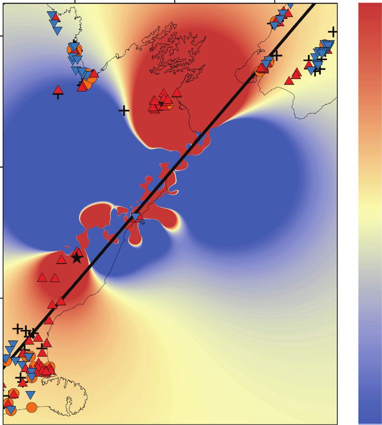
2                                                                                                                             Geofluids

     Earthquakes are known to induce groundwater level                  were classified on the basis of depth and local aquifer pres-
changes with varying amplitude, duration, and polarity of               sures, using the terms “water-table,” “nonflowing,” and
response (e.g., [18–20]). Earthquake-induced static and                 “flowing artesian” based on the groundwater level relative
dynamic stresses (e.g., [21]) and local hydrogeological factors         to ground prior to the earthquake at each site. The majority
[22] influence groundwater level responses. In this first                 of wells are less than 100 m deep, which are shallow in com-
report on the Kaikōura earthquake’s hydrogeological effects,             parison with those considered in international studies (e.g.,
we document an extensive dataset of groundwater level                   [32, 33]). Screens typically range from 1 to 10 m in length,
responses in order to assess the level to which earthquake-             and well diameters generally vary from 50 to 300 mm, but
driven and local hydrogeological factors contributed to the             overall, the construction method and well completion do
national scale groundwater level response. This earthquake              not vary appreciably across the regions, resulting in similar
hydrology dataset is the most extensive compiled in New                 style of earthquake-induced responses. The aquifers mostly
Zealand, surpassing that compiled by Cox et al. [23] follow-            occur in young sedimentary deposits that have varying levels
ing the Mw 7.1 Darfield (Canterbury) earthquake, and is of               of consolidation, with few aquifers in igneous or metamor-
comparable size to datasets compiled following the 1999                 phic rocks. A notable exception are the geoengineered schist
Mw 7.5 Chi-Chi earthquake in Taiwan [24, 25]. In compari-               landslides in Cromwell Gorge [34], which have fracture per-
son to other case studies, the Kaikōura earthquake dataset              meability and water tables that have been displaced from
is also significant as it includes groundwater level responses           their natural condition by drainage tunnels. In contrast to
collated from a variety of hydrogeological settings.                    these examples from New Zealand, many international stud-
                                                                        ies of earthquake hydrology provide datasets on aquifers in
2. New Zealand Hydrogeology                                             well-consolidated and crystalline rocks (e.g., [35–37]).
                                                                            We gathered rainfall and atmospheric pressure data from
There are a wide variety of compositionally diverse aquifers            65 climate stations, which are managed and maintained by
in New Zealand that were formed in a range of depositional              the National Institute for Water and Atmospheric Research.
environments, mainly during the Tertiary and Quaternary                 Barometric corrections were applied where necessary using
geological periods. Sedimentary aquifers were formed from               data from the nearest climate station, leaving monitoring well
terrestrial (e.g., glacial, aeolian), shallow (e.g., deltaic, carbon-   water level data relative to water level only. Rainfall data were
ate), and deep marine sedimentary deposits, with mixed clast            qualitatively compared to groundwater level data before, dur-
composition reflecting the varied source rock geology [26].              ing, and after the Kaikōura earthquake, to assess any effect on
Transgression/regression sequences created overlaps of ter-             observed water level changes.
restrial and marine deposits in coastal areas [27], resulting               Earthquake-induced water level changes can be split into
in large variations in vertical and horizontal permeability             coseismic and postseismic components relative to the period
and storage capacity [28]. There are also volcanic aquifers             of shaking at the monitoring site. The primary responses
of ignimbrite and scoriaceous deposits formed in the central            observed in this study were postseismic, as most of the
North Island from Taupō Volcanic Zone caldera eruptions                 records were collected at 15-minute intervals, the first occur-
and basalt flows, respectively. Groundwater is also stored in            ring after the shaking had stopped. Water level changes were
Mesozoic-Cretaceous metamorphic bedrock that forms                      classified as either having no response, responding tran-
mountain ranges in both North and South Islands but is sel-             siently and returning to preearthquake levels within two
dom utilised for water supplies due to the low permeability             hours, or responding persistently (increasing or decreasing)
and yield of the bedrock [26].                                          and reequilibrating at a new postearthquake level lasting sev-
                                                                        eral days or longer (Figure 2). For each water level change,
3. Hydrological and Seismic Data                                        the polarity, amplitude, and duration until reequilibrated or
                                                                        returned to preearthquake levels were recorded. The ampli-
The hydrological monitoring infrastructure in New Zealand               tude of persistent water level changes was estimated from
is extensive due to the country’s heavy reliance on groundwa-           the difference between the reequilibrated and preearthquake
ter for agriculture [26]. Regional councils manage and main-            groundwater level. At this longer time scale (than coseismic
tain networks of boreholes instrumented by data loggers and             responses) and since most wells are specifically for monitor-
pressure sensors that measure groundwater levels, represent-            ing (rather than production), we assume that any wellbore
ing piezometric levels. The monitoring infrastructure is not            storage effect has already passed in water table wells, but
evenly distributed as groundwater tends to be extracted from            some observed responses in confined aquifers could result
the most permeable areas, predominantly gravel aquifers,                from changes in transmissivity. Water level time series were
and pumping test data are not readily available. Where                  removed from the analysis in cases in which earthquake-
repeated pumping test data are available, the inferred trans-           induced damage to the well compromised or prevented the
missivities are ambiguous [29], highly variable [30], and               recording of water level.
catchment dependent [31].                                                   The following general terms have been adopted for mon-
     We collected groundwater level time series data spanning           itoring wells with respect to earthquakes [38]: “near field”
the Kaikōura earthquake from 433 monitoring wells distrib-              denotes wells within one rupture fault length and “intermedi-
uted throughout New Zealand (Figure 1). Groundwater                     ate field” represents wells from one to ten rupture fault
levels are sampled at intervals ranging from one minute to              lengths away. Considering the Kaikōura earthquake rupture
three hours, with 15 minutes being the most common. Wells               zone extends ~180 km northeast of the epicentre (Figure 1),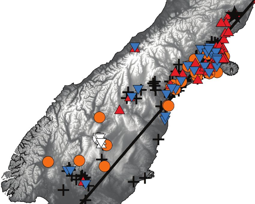
Geofluids 3
(a) (b) (c)
35º S
42º S
a a 40º S
N
100 km
174º E
45º S
N
400 km
170º E 180º
Earthquake (a) Seismic sites (b) Hydrological sites (c)
Kaikōura Mw 7.8 Strong motion Climate station
Fault rupture Broadband Monitoring well
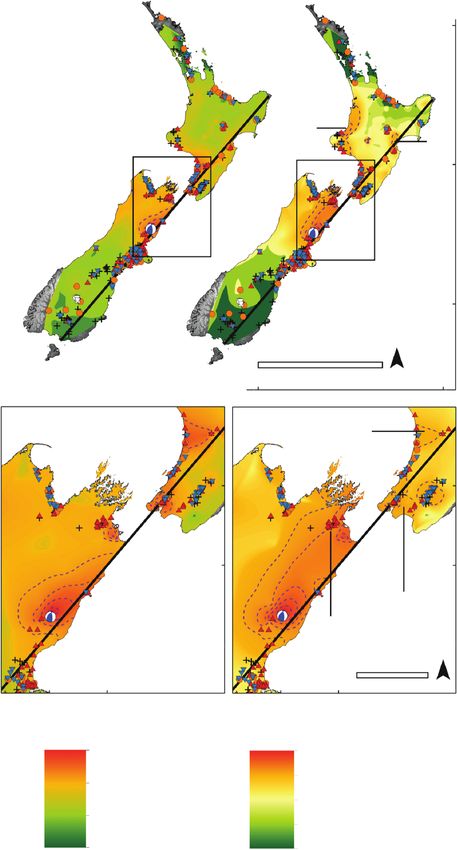
Figure 1: Spatial distribution of the hydrological and seismic dataset that recorded the 2016 Mw 7.8 Kaikōura earthquake. (a) Kaikōura
earthquake focal mechanism [5] and surface rupture zone [13]. (b) 306 seismic stations (strong motion and broadband) recorded the
Kaikōura earthquake. (c) Water level data were collected from 433 monitoring wells, and rainfall and atmospheric pressure were collected
from 65 climate stations, which spanned the earthquake interval. Monitoring wells in Cromwell Gorge are highlighted differently.
the near field region extends ~360 km to the north and earthquakes in southern California [41], the term is accepted
~180 km to the south of the epicentre (Figure 2). internationally and used for seismo-hydrological phenomena
We compiled all available New Zealand seismic record- (e.g., Weingarten and Ge, 2013; [36, 42, 43]). Of the well
ings of the Kaikōura earthquake from 306 strong motion water levels observed, 146 showed a persistent increase, 91
and broadband seismic stations. The seismic stations are part exhibited a persistent decrease, and 69 displayed a transient
of the National Seismograph Network and Strong Motion change. At 127 wells, there was no observed change. In the
Network (http://geonet.org.nz). Instrument responses were near field, approximately two-thirds of the persistent water
corrected, and a band-pass filter with transition bands of level changes observed were increases. In the intermediate
0.10-0.25 Hz and 24.50-25.50 Hz was applied. Shaking field, changes were roughly equally split between increases
parameters, peak ground velocity (PGV) and acceleration and decreases. The largest persistent water level increase
(PGA), were calculated at each seismic station and interpo- was ~3.5 m and the largest decrease was ~3.3 m, both of
lated to the monitoring wells using the nearest neighbour which were observed in Cromwell Gorge. In simple terms,
interpolation method [39]. In the absence of borehole seis- water level changes in the near field had larger amplitudes
mometers, we make an implicit assumption that surface than those in the intermediate field. The time taken for water
shaking observed at the seismograph sites, interpolated levels to reequilibrate at new postearthquake levels generally
locally as parameters at the well site, is applicable over the ranged from 10 minutes to two hours, with a median time of
depth of the wells since they are mostly shallow. 65 minutes and the longest time of 100+ days (Cromwell
Gorge).
4. Groundwater Level Changes Induced by the
Kaikōura Earthquake 5. The Influence of Earthquake-Driven Factors
on Water Level Changes
The Kaikōura earthquake induced groundwater level changes
across New Zealand in the near and intermediate fields. 5.1. Earthquake-Induced Static Stress Changes. Static stress
Water level changes were recorded at 433 sites from 4 to changes are permanent and decay rapidly with distance (r)
850 km from the earthquake epicentre (Figure 2), at seismic at ~1/r 3 , meaning that they are most significant in the near
energy densities [40] ranging between 10–2 and 105 J/m3 field (Figure 4, [44, 45]). Earthquake-induced static stress
(Figure 3). Although the relationship of seismic energy den- changes imposed on the surrounding crust cause volumetric
sity, magnitude, and epicentral distance was derived from strain changes within aquifer systems. Studies have suggested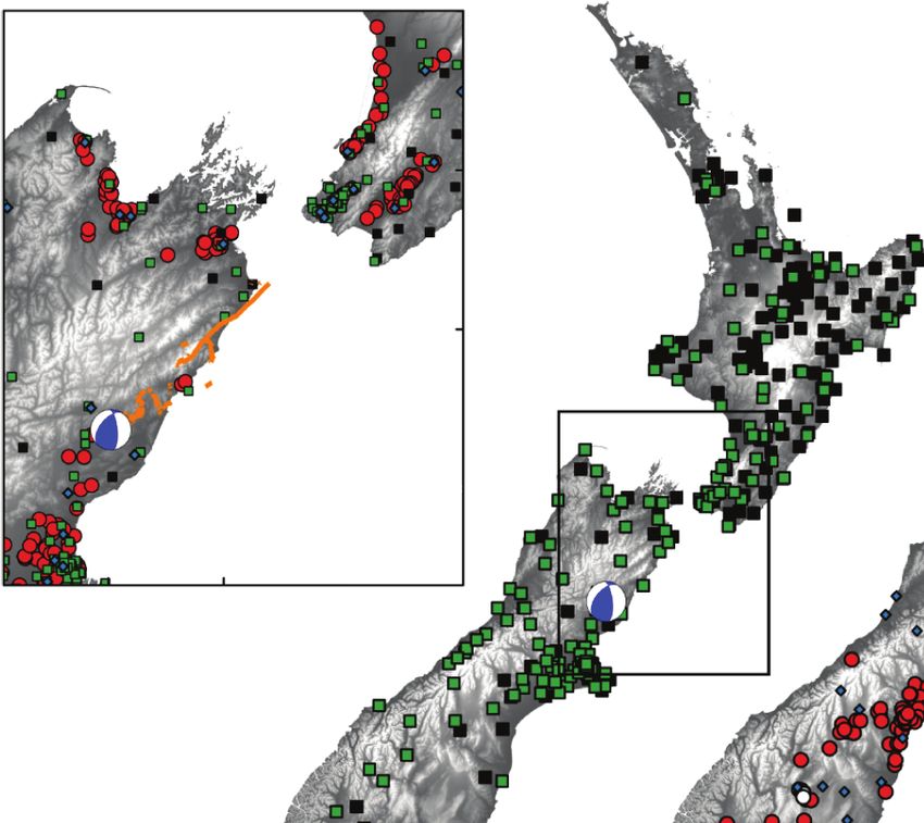
4                                                                                                                                                     Geofluids

                          88
    Water-level (m)

                                                                                                                                                      35 º S
                          86

                                       Persistent increase
                               −12             −6             0          6       12
                                           Time relative to earthquake (hours)

                                                       (a)
      Water-level (m)

                          22.0

                          21.5
                                       Persistent decrease
                                 −12            −6            0          6       12
                                          Time relative to earthquake (hours)

                                                       (b)                                                                                            40º S

                          74.6
        Water-level (m)

                          74.8

                                  Transient
                                 −12            −6            0          6       12
                                           Time relative to earthquake (hours)

                                                                                                                                                eld

                                                                                                                                               eld
                                                        (c)

                                                                                                                                            -fi

                                                                                                                                           e-fi
                                                                                                                                          ar

                                                                                                                                        iat
                                                                                                                                       Ne

                                                                                                                                      ed
                                                                                                                                     m
                                                                                                                                  ter
                                                                                                                                In

                                                                                                                                                      45º S

                                                                                                           170º E                 175º E

                                                                                      Earthquake                     Response (Cromwell Gorge)
                                                                                         Mw 7.8 Kaikoura                  Increase
                                                                                      Response                            Decrease
                                                                                         Increase                         Transient
                                                                                         Decrease                    Transect
                                                                                         Transient                        SW-NE transect
                                                                                         No response                      Near/Intermediate field
                                                                                                                    (d)

Figure 2: Three examples of earthquake-induced groundwater level responses characterised and the spatial distribution of water level
changes induced by the 2016 Mw 7.8 Kaikōura earthquake. (a) Persistent water level increase. (b) Persistent water level decrease. (c)
Transient water level change. (d) Spatial distribution. Sampling intervals are 15 minutes (a, b) and 5 minutes (c). Responses in Cromwell
Gorge are highlighted separately. The thick black line shows a transect approximately parallel to the long axis of the surface rupture zone;
see Figure 8 for water level changes along this transect.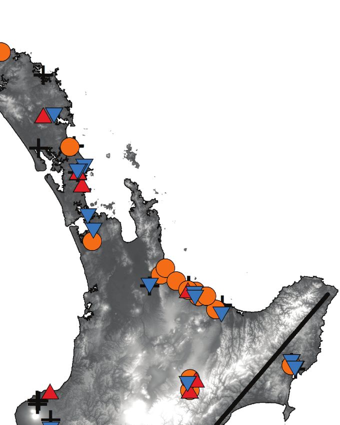
Geofluids                                                                                                                                                          5

                                                 104

                                                 103
                  Distance from epicentre (km)

                                                 102
                                                            −5
                                                           10

                                                            −3
                                                 101       10

                                                            −1
                                                           10                                                    Kaikōura Mw 7.8
                                                                  1                3                   5
                                                                 10               10                  10           (this study)
                                                 100
                                                       3          4           5             6              7           8              9            10
                                                                                        Earthquake magnitude

                  Global case studies                                   New Zealand case studies                   Other studies
                                                 1999 Chi-Chi Mw 7.3         2010 Darfield Mw 7.1                       Global data catalogue
                                                 2006 Hengchun Mw 7.0        2011 ChCh Mw 6.2                           Devils Hole
                                                 2008 Wenchuan Mw 7.9        2011 ChCh Mw 5.3                           Cromwell Gorge
                                                 2011 Tohoku Mw 9.0          2011 ChCh Mw 6.0                           Seismic energy density (J/m3)
                                                 2013 Lushan Mw 6.6          2016 Kaikōura Mw 7.8
                                                                             2016 Kaikōura Mw 7.8 (Cromwell Gorge)

Figure 3: Earthquake magnitude as a function of distance from epicentre, where a groundwater level response was observed. We collated New
Zealand and global case studies. New Zealand studies include 2010 Darfield Mw 7.1 [23]; 2011 Christchurch Mw 6.2, 5.3, 6.0 [104]; and
Cromwell Gorge [34]. International studies include 1999 Chi-Chi Mw 7.3 and 2006 Hengchun Mw 7.0 [82]; 2008 Wenchuan Mw 7.9 [37,
105]; 2011 Tohoku Mw 9.0 [106]; and 2013 Lushan Mw 6.6 [33]. Also included is a worldwide compilation of groundwater responses [84],
responses from the extremely sensitive Devils Hole [75], and seismic energy density contours in J/m3 [40]. ChCh = Christchurch.

that volumetric strain changes cause water level changes (e.g.,                                     increases (n = 98), and static stress-induced tensional
[46–49]). The contractional and dilatational volumetric                                             changes between 101 and 102 kPa occurred generally with
strain changes are inferred to increase and decrease water                                          water level decreases (n = 13). Compressional changes
levels, respectively, with predictable amplitudes (e.g., [50]).                                     smaller than 101 kPa occurred more frequently with
However, several fault lengths away from the epicentre, water                                       decreases in water level (n = 53) than increases (n = 39),
level changes are commonly larger in amplitude and incon-                                           although the larger amplitudes were mostly increases. At
sistent in water level change polarity (increase/decrease) with                                     lower than ±102 kPa regardless of the sign of σkk , some water
model predictions [38, 51, 52].                                                                     levels did not respond. Significant (>1 m) water level changes
     To calculate the mean static stress changes (σkk ), we used                                    were observed in Cromwell Gorge, where σkk was less than
the slip distribution of Clark et al. [16] to calculate the inter-                                  −100 kPa (Figure 5).
nal strain field based on the formulation of Okada [53] at
500 m depth across the epicentral region. Using a Poisson’s                                         5.2. Earthquake-Induced Dynamic Shaking. Dynamic stress
ratio of 0.25 and a shear modulus of 30 GPa, we then convert                                        changes caused by the passage of seismic waves are short-
the strain to stress at 500 m depth. Modelled fault slip geom-                                      lived and decay at ~1/r 5/3 , meaning that they can be signifi-
etries for the 21 ruptured faults were based on the surface                                         cant from the near to far field [44, 45]. Dynamic stress-
rupture field [15] and geodetic data. Positive σkk indicates                                         induced deformation depends on loading rates and cycles
tensional stress changes, and negative σkk indicates compres-                                       of inertial forces [45] and is influenced by rupture directivity
sional stress changes.                                                                              and radiation patterns [40].
     As expected, σkk was most significant in the near field                                              Peak ground velocity (PGV) reflects the majority of
(Figure 4). In total, 386 wells were in areas of contraction,                                       energy in seismic ground motion [40] and is easily measur-
where σkk ranged from −0.2 to −18,800 kPa. 47 wells were                                            able. PGV can be related to the Modified Mercalli Intensity
in areas of dilatation, where σkk ranged from 0.7 to 120 kPa                                        scale (e.g., [54]) and is a potential indicator for engineers in
(Figure 5). Static stress-induced compressional changes                                             seismic assessment methods (e.g., [55]). PGV has been com-
larger than 101 kPa occurred predominantly with water level                                         pared to water level changes (e.g., [35, 37]) and is related to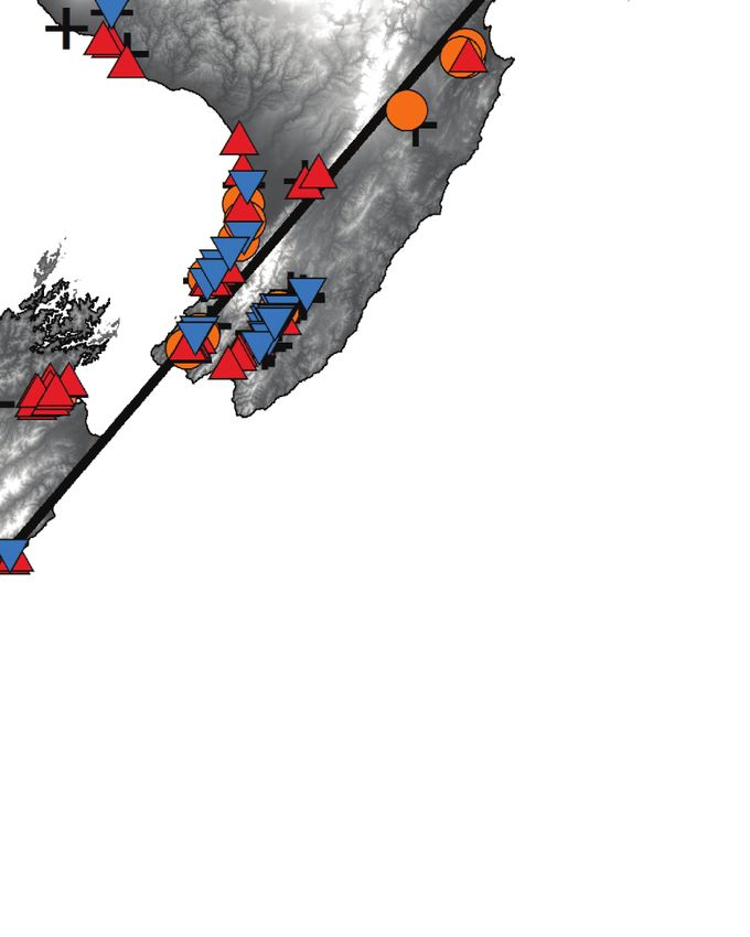
6                                                                                                                               Geofluids

                                                                                        Mean static
                                                                                    stress change (휎kk)
                                                  173º E      174º E       175º E    Compressional
                                                                                               −100 kPa
                                   41º S

                                   42º S

                                                                                                  0 kPa

                                   43º S

                                                                                                100 kPa
                                                                                        Tensional
                                                                                        N

                                     Earthquake                          100 km
                                           Mw 7.8 Kaikōura
                                     Response
                                           Increase
                                           Decrease
                                           Transient
                                           No change
                                     Transect
                                           SW-NE transect

Figure 4: Spatial distribution of water level changes and mean static stress changes (σkk ) induced by the Kaikōura earthquake. Red colours
indicate compression; blue colours indicate tension. A transect through the surface rupture zone and the majority of monitoring wells is
shown in Figure 8.

peak dynamic stress, which has been utilised in permeability           considerations of changes in stress and uses the horizontal
enhancement experiments (e.g., Roberts, 2005; [56]).                   (geometric mean) peak ground acceleration (PGA) [66, 67].
Dynamic stresses are thought to control the incidence of               PGA also correlates with the amplitude and occurrence
shear-induced consolidation and dilatation [57–59], vertical           of groundwater level changes [68, 69]. We compared the
(e.g., [40, 60, 61]) and horizontal (e.g., [62]) enhancement           horizontal (geometric mean) PGA to groundwater level
of permeability. Peak dynamic stress (σD , GPa) can be                 changes. Comparing both PGV and PGA to groundwater
expressed [63] as                                                      level changes allowed an assessment of whether velocity
                                                                       or acceleration was the better indicator for determining
                                 μS PGV                                the polarity, amplitude, and/or duration of water level
                          σD ~                                  1      change.
                                    vs
                                                                           PGV and PGA were the highest in the near field, adjacent
                                                                       to the fault rupture, and notably high in areas of Marlbor-
in terms of the shear modulus (μS , GPa), shear wave velocity          ough, Wellington, Manawatu-Wanganui, Taranaki, and
at the monitoring well (vs , m/s), and maximum peak ground             Hawkes Bay regions. The extent of the fault rupture to the
velocity (PGV, m/s). The maximum PGV of horizontal and                 north of the epicentre and the northward rupture directivity
vertical motions has been used here as a proxy for dynamic             of the earthquake resulted in a slower decay of PGV and PGA
stress (equation (1), [62, 64, 65]).                                   north of the epicentre and a more rapid decay of PGV and
    The assessment of liquefaction, an earthquake-induced              PGA south of the epicentre. The higher PGV and PGA north
hydrogeological response (e.g., [40]), is typically based on           of the epicentre correlate with more frequent larger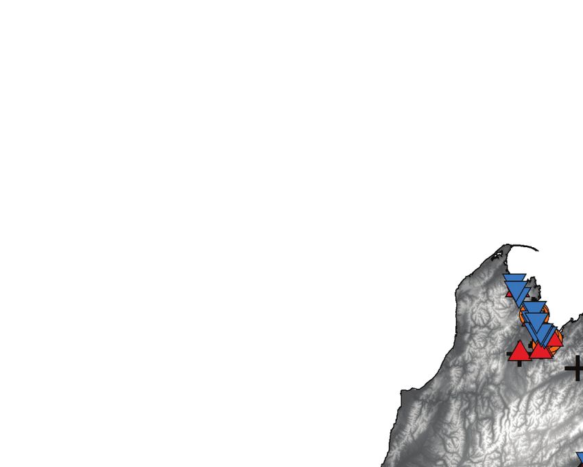
Geofluids                                                                                                                                                    7

                     Water-level change (m)
                                               3
                                               2
                                               1
                                               0
                                              −1
                                              −2                                                              ii
                                              −3                                    i                                 Compressional (−휎kk)

                                                                 100        101                     102             103                  104
                                                                       Absolute mean static stress change (휎kk, kPa)

                                                                                        (a)
                     Water-level change (m)

                                               3
                                               2
                                               1
                                               0
                                              −1
                                              −2
                                                                                              i
                                              −3                                                                               Tensional (+휎kk)
                                                                 100        101                     102             103                  104
                                                                       Absolute mean static stress change (휎kk, kPa)

                                                   Response                                        Response (Cromwell Gorge)
                                                      Increase                                        Increase
                                                      Decrease                                        Decrease
                                                      Transient                                       Transient
                                                      No response
                                                                                        (b)

Figure 5: The relationship between earthquake-induced mean static stress changes (σkk ) and water level changes. (a) Static stress-induced
compressional stress changes. High areas of compressional stress changes include (i) Wellington and Canterbury and (ii) Marlborough.
(b) Static stress-induced tensional stress changes. High areas of tensional stress changes include (i) Tasman.

amplitude water level changes. North of the epicentre, 60% of                                     to an earthquake, some monitoring wells respond with
water levels changed persistently, while south of the epicentre                                   larger amplitudes of water level change than others at
48% of water levels changed persistently (Figures 6–8).                                           the same epicentral distance. Aquifer properties are likely
     At monitoring wells, the PGV ranged from 0.002 to                                            to partly control earthquake-induced water level changes.
0.9 m/s and the PGA ranged from 0.01 to 11.8 m/s2. Above                                          The higher the transmissivity of the formation, the more
a PGV of ~0.3 m/s and a PGA of ~2 m/s2, the majority of per-                                      the well water level change will be reflective of the forma-
sistent water level changes were increases, and the median                                        tion pressure change, with the time taken for water levels
response reequilibration times were 1455 and 585 minutes,                                         to reequilibrate or return to preearthquake levels being
respectively. Below a PGV of ~0.3 m/s and a PGA of                                                governed by flow properties [70].
~2 m/s2, there was no preferred polarity, and the median                                              Since PGA differentiates polarity behaviour more clearly
response reequilibration time was 75 minutes below both                                           than PGV (Figure 7) and that earthquake-induced dynamic
thresholds. PGA differentiates polarity behaviour more                                             shaking occurred at all monitoring wells, we scaled the
clearly than PGV, with 32 persistent water level increases                                        absolute water level change amplitudes (WLC, m) to the
above ~2 m/s2, compared to 11 persistent water level                                              horizontal (geometric mean) PGA (m/s2) experienced at
increases above ~0.3 m/s. Some monitoring wells that experi-                                      each monitoring well (WLC/PGA, s2). To further under-
enced low levels of shaking showed a larger water level                                           stand the local hydrogeological factors in contributing to
change than wells that experienced high levels of shaking,                                        water level changes, we compared WLC/PGA to the depth
such as wells in Cromwell Gorge (Figure 7). This may be                                           of monitoring well and to the average shear wave velocity
due to local hydrogeological conditions that partly contribute                                    as a representation of the degree of confinement and
to the characteristics of water level changes.                                                    expected dynamic rock strength behaviour at each site.

6. The Influence of Local Hydrogeological                                                         6.1. Depth. Earthquake-induced water level changes vary
   Factors on Water Level Changes                                                                 with the degree of confinement in aquifer formations. Water
                                                                                                  level changes in unconfined aquifers are generally smaller
Although distance from the epicentre provides a rough                                             than those in confined/semiconfined aquifers [50], as a result
approximation of how a monitoring well may respond                                                of the specific yield of unconfined aquifers being higher than
8 Geofluids
Earthquake
(a) (c)
35º S
Mw 7.8 Kaikōura
Transect
SW-NE transect
Response
Increase
Decrease
Transient i
No change ii
Response
b d 40º S
(Cromwell Gorge)
Increase
Decrease
Transient
45º S
N
500 km
170º E 180º
(b) 0.2 (d)
iii
1
1
1
0.2
2
0.4
8
2
0.2 6
0.2 42º S
4
42º S
0.4 4
6
0.6 8
0.8 10 ii
i
N
100 km
174º E 174º E
(a, b) (c, d)
Maximum Horizontal (geometric
PGV (m/s) mean) PGA (m/s2)
100 101
100
10−1
10−1
10−2
10−2
10−3 10−3
Contour (m/s) Contour (m/s2)
Figure 6: Spatial distribution of water level changes, maximum PGV, and horizontal (geometric mean) PGA induced by the 2016 Mw 7.8
Kaikōura earthquake. Spatial distribution of the water level changes on a national scale compared to PGV (a) and PGA (c). Notably high
levels of shaking occurred in the (i) Taranaki and (ii) Hawkes Bay regions. Spatial distribution of water level changes in central New
Zealand as a function of PGV (c) and PGA (d). Notably high levels of shaking occurred in the (i) Marlborough, (ii) Wellington, and (iii)
Manawatu-Wanganui regions. Red colours indicate high levels of PGV and PGA; green colours represent low levels of PGV and PGA. A
transect through the surface rupture zone and the majority of monitoring wells is shown in Figure 8.
Geofluids                                                                                                                                                                   9

                                                                                                                                            0.3 m/s
               Absolute water-level change amplitude (m)

                                                           100

                                                           10−1

                                                           10−2

                                                                                                         No preferred polarity                        Predominantly
                                                           10−3
                                                                                                                                                         increases

                                                                                 10−2                           10−1                                                100
                                                                                           Maximum PGV (m/s)

                                                                                                         (a)

                                                                                                                               2 m/s2
               Absolute water-level change amplitude (m)

                                                           100

                                                           10−1

                                                           10−2

                                                                                                                                        Predominantly
                                                           10−3                                 No preferred polarity                     increases

                                                                   10−2            10−1                         100                                           101
                                                                                                                           2
                                                                                   Horizontal (geometric mean) PGA (m/s )

                                                                  Response       Response (Cromwell Gorge)             Kernel density estimate
                                                                     Increase       Increase                                   Increase
                                                                     Decrease       Decrease                                   Decrease
                                                                     Transient      Transient                                  Transient
                                                                     No change                                                 No change

                                                                                                         (b)

Figure 7: Absolute water level change amplitude as a function of (a) maximum PGV and (b) horizontal (geometric mean) PGA. Above a PGV
of ~0.3 m/s and a PGA of ~2 m/s2, water level changes were predominantly increases.

the storativity of confined aquifers [71]. Changes in monitor-                                                  mean stress (σkk , GPa), and the magnitude of pore pressure
ing well water levels in unconfined aquifers reflect the (de)wa-                                                 change is governed by Skempton’s coefficient (B) [50].
tering process of pore spaces above/below the water table,                                                         We used the depth of each monitoring well (4 m to
which forms the aquifer upper boundary. Changes are also                                                       1.4 km) as a first-order proxy for the degree of confinement
influenced by well storage effects, the impact of which                                                          of the aquifers studied. The monitoring wells are generally
increases with decreasing transmissivity [50]. Assuming                                                        shallow with the median depth being 24 m. At any depth,
undrained conditions [64], changes in confined aquifer pore                                                     WLC/PGA typically varies by two orders of magnitude. Gen-
pressure (p, GPa), given by p = −Bσkk /3, are proportional to                                                  erally, the deeper the monitoring well, the more sensitive the
10 Geofluids
4
2
change (m)
Water-level
0
−2 Fault rupture length
−4
(a)
Horizontal (geometric
0.8 8
mean) PGA (m/s )
Intermediate-field Near-field Intermediate-field
2
0.6 6
PGV (m/s)
Maximum
0.4 4
0.2 2
0 0
(b)
change (휎kk, MPa)
Mean static stress
−20
Compressional
0
Tensional
20
−600 −400 −200 0 200 400 600
SW NE
i ii iii iv v vi vii
Distance along transect (from epicentre) (km)
Water-level change (a) Earthquake shaking (b)
Response Response (Cromwell Gorge) Maximum PGV
Horizontal (geometric mean) PGA
Increase Increase
Static stress change (c)
Decrease Decrease
Mean stress change
Transient
Transient
No response
(c)
Figure 8: A cross section of the Kaikōura earthquake-induced (a) groundwater level changes, (b) maximum PGV and horizontal (geometric
mean) PGA, and (c) mean static stress changes (σkk ). Locations of interest are (i) Cromwell Gorge monitoring wells, (ii) earthquake epicentre,
(iii) Marlborough region, (iv) Cook Strait, (v) Wellington, (vi) Manawatu-Wanganui, and (vii) Hawkes Bay regions. The cross section goes
through the Kaikōura surface rupture zone and the majority of monitoring wells.
well was to water level change. A similar observation was shaking [74]. Sensitive hydrological sites screened in well-
recorded by Rutter et al. [29], who found that water level consolidated or crystalline rocks can respond to teleseismic
changes occurred more consistently in wells of greater than earthquakes over 1000 km away and typically do so with
80 m depth, compared to shallower wells. At depths less than hydroseismograms (e.g., [32, 36, 62, 75, 76]). Where static
10 metres, WLC/PGA broadly ranged from ~10–3 to 10–1 s2. and dynamic stresses are insignificant, hydrogeological factors
At depths between 10 and 100 metres, WLC/PGA mostly must partly control the hydrological response. The geoengi-
varied from ~10–2 to 100 s2. Deeper than 100 metres, neered schist landslides of Cromwell Gorge respond hydrolog-
WLC/PGA largely fluctuated from ~10–1 to 101 s2. All types ically with large amplitude, although static and dynamic
of water level changes were observed over the entire depth stresses are insignificant (Figure 8). Where static and dynamic
range as shown by the kernel density estimate. Monitoring stresses are significant, hydrogeological factors may influence
wells in Cromwell Gorge geoengineered landslides were gen- hydrological responses but are probably less substantial. In
erally the most sensitive (Figure 9). The WLC/PGA for the near field, responses are not entirely consistent with the
unconfined water table aquifers does not exceed 100. magnitude of static or dynamic stresses (Figure 8).
To reflect the varied hydrogeological conditions of the
6.2. Shear Wave Velocity. Seismic waves attenuate differently aquifers studied, we used site average shear wave velocity
in different rock types [38], and it is therefore unsurprising (Vs30, m/s) over depths between 0 and 30 m [77] at each
that hydrogeological factors partly control earthquake- monitoring well. Shear wave velocities range from 40 to
induced groundwater level changes. Site effects and varying 1040 m/s, representing very soft soil to weak rock, respec-
crustal structures have differing efficiencies of dynamic shak- tively [78]. Vs30 is typically towards the lower end of this
ing [40]. Saturated unconsolidated media damp high- range, the median Vs30 being 225 m/s, representative of deep
frequency motions, while amplifying lower frequencies [25, soil. At any Vs30, WLC/PGA varied over three orders of
72, 73]. In contrast, consolidated/crystalline aquifer material magnitude. Broadly, as Vs30 increases, WLC/PGA increases.
amplify high-frequency shaking more than low-frequency When Vs30 ranged between 0 and 270 m/s, WLC/PGAGeofluids 11
101
Depth (m)
102
103
10–3 10–2 10–1 100 101
WLC amplitude normalised by geometric mean horizontal PGA
Well Response Kernel density estimate
Increase Water-table Increase
Water-table
Decrease Non-flowing artesian Decrease
Non-flowing artesian
Transient Flowing artesian Transient
Flowing artesian
No change No change
Figure 9: WLC/PGA as a function of monitoring well depth. Coloured according to monitoring well type (water-table, nonflowing artesian,
and flowing artesian). The deeper the monitoring well, the more sensitive the well was to water level change. All types of water level response
(increase, decrease, transient, and no change) were observed over the entire depth range. Artesian wells commonly show water level increases
at high WLC/PGA.
typically ranged from ~10–3 to 100 s2. When Vs30 was close to vu value of ~9 GPa. Therefore, σkk of ±100 and ±101 kPa
1000 m/s, WLC/PGA was mostly between ~10-2 and 101 s2. predicts a ~10 cm and ~1 m water level change, respectively.
There is no correlation between polarity of water level However, most wells with σkk of12 Geofluids
Figure 10: WLC/PGA as a function of site classification [78]. Site classifications are converted from Vs30 [77]. Monitoring well depths
shallower than 30 m have larger opaque symbols as Vs30 is representative. Monitoring well depths deeper than 30 m have smaller
transparent symbols as Vs30 is less representative.
greatly exceed a threshold of ~10–4 [58], shear-induced dila- colloidal particles [90]. It has been postulated that dislodging
tation occurs [83]. Groundwater levels can decrease persis- of colloidal particles from preferential flow pathways may
tently as a result of the decrease in pore pressure and enhance horizontal permeability ([62, 84, 91] [29]). The
increase in porosity [84]. Shear-induced dilatation may have change in water level may originate in close proximity to a
occurred in close proximity to the Kaikōura earthquake fault local pressure source, which could be produced by liquefac-
rupture. However, as a result of the numerous landslides [85] tion [92], or elevated hydraulic heads [93]. Earthquake-
and limited number of monitoring wells adjacent to the fault induced flow velocities may be strong enough to dislodge
rupture, it is unclear to what extent shear-induced dilatation colloidal particles [90]. Laboratory experiments on pore
may or may not have occurred. unclogging [56, 94] and groundwater colour changes [95]
Shear-induced consolidation and liquefaction [40, 83] support permeability enhancement by dislodging colloids.
occur at lower cyclic shear strains, still exceeding ~10–4 [57, The location of permeability enhancement could occur either
59]. Shear-induced consolidation predicts that water levels up- or down-hydraulic head gradient of a monitoring well. If
increase persistently as a result of dynamic shaking, due to enhancement occurs up-hydraulic head gradient of a moni-
consolidating the sediment within an aquifer and decreasing toring well, water level in the well would increase, as more
porosity [83]. The threshold at which persistent water level flow is directed towards the well. If enhancement occurs
increases predominantly occurred was at a horizontal (geo- down-hydraulic head gradient, water level in the well would
metric mean) peak ground acceleration (PGA) of ~2 m/s2 decrease, as flow is directed away from the well. Therefore,
and a maximum peak ground velocity (PGV) of 0.3 m/s. if a sufficiently large number of observations are made, the
PGA differentiated persistent water level increases from permeability enhancement model would predict a statisti-
other response types more clearly than PGV (Figure 7). cally random occurrence in the polarity of the water level
Dynamic shaking also caused liquefaction to occur in the change [84]. In this study, there was roughly an equal num-
Marlborough [86, 87] and Wellington [17, 88, 89] regions. ber of persistent water level increases and decreases at accel-
These areas experienced a PGA exceeding ~2 m/s2 and had erations lower than PGA of ~2 m/s2, with water level change
predominantly persistent water level increases. amplitudes generally less than 1 m. Furthermore, flowing
At low thresholds of dynamic shaking, earthquake- artesian wells have positive responses in 33 out of 39
induced flow velocities may be strong enough to dislodge instances (see Supplementary Materials). This is consistentGeofluids 13
with the model of enhanced permeability. Persistent water water level changes occurred mainly below a PGA of
level changes may have occurred above a PGA of ~2 m/s2 ~2 m/s2 with small amplitudes of water level changes,
as a result of enhanced permeability but may be concealed (Figure 7), and are likely to be a result of poroelastic deforma-
by larger amplitude changes caused by shear-induced tion (e.g., [64, 92]).
consolidation [38].
Water level changes caused by dislodging colloidal parti- 7.3. Local Hydrogeological Factors. Although shear-induced
cles may be described as gradual sustained changes because consolidation and enhancement of permeability are likely
the response reequilibration time to new postearthquake to have partly contributed to the polarity and occurrence
levels depends on the distance between the source of the of water level changes, the amplitude of water level change
blockage and the monitoring well [62, 92]. Water level had a weak correlation with PGA (Figure 7). Some moni-
changes caused by consolidation are more likely to be toring wells were more sensitive to water level changes than
described as abrupt changes because immediate changes in others at similar ground accelerations, which may be par-
pore pressure occur as a result of an undrained volumetric tially a result of hydrogeological factors. 400 km south of
change around the well [38]. In this study, the median persis- the epicentre (Figure 8), monitoring wells in Cromwell
tent response reequilibration time for monitoring wells that Gorge screened in schist rock exhibited water level changes
experienced a PGA above ~2 m/s2 (n = 33) was 585 minutes, of ~±3 m. Yet, monitoring wells within 200 km of Cromwell
while below a PGA of ~2 m/s2 (n = 204) was 75 minutes. The Gorge, mainly screened in unconsolidated deposits,
two populations of response times were statistically different. responded persistently with small amplitudes of less than
Shear-induced consolidation may occur on a large scale (km) 1 m. Cromwell Gorge monitoring wells are known to be
[83], as the threshold of shaking is likely to be exceeded over sensitive to hydrological change from multiple earthquakes.
a wide area near the earthquake epicentre. However, perme- Cromwell Gorge groundwater levels are depressed below
ability enhancement caused by dislodging of colloids may equilibrium levels by pumping and gravity drainage due
occur more frequently on a small scale (m) [62] in prefer- to infrastructure, and the sensitivity may in part reflect
ential flow pathways. The response time may reflect the anthropogenic modification of the groundwater regime
scale at which these processes occur at but should not be [34]. Devils Hole, Nevada, is another example of a site that
considered definitive. is sensitive to change, with responses occurring at low seis-
International case studies have shown that undrained mic energy densities of 10–6 J/m3 [75]. Since there is a dis-
consolidation/dilatation is the dominant mechanism in the parity between the global dataset [84] and case studies
near field, with enhanced permeability being dominant in (Figure 3), it is possible that response thresholds vary
the intermediate field [38]. In the field, seismic energy densi- widely as a result of hydrogeological factors. Different
ties larger than ~101 J/m3 are above the threshold for catchment responses may also affect the hydrological
undrained consolidation, with sensitive sites experiencing response to the earthquakes (e.g., [31]).
consolidation above ~10–1 J/m3 [38, 96]. For the Chi-Chi Depth is positively correlated with WLC/PGA
and Hengchun earthquakes, the transition from consolida- (Figure 9), which concurs with studies that observed pro-
tion to enhanced permeability was inferred at ~101 J/m3 nounced earthquake-induced water level changes in deeper
[84]. In this investigation, that equates to an epicentral dis- confined aquifers compared to shallow unconfined aquifers
tance of 100 km (near field), where water level changes were [29, 50, 98, 99]. This is because the specific yield of uncon-
still predominantly increasing (Figure 8). The terms seismic fined aquifers is higher than the storativity of confined
energy density [40], near and intermediate fields [38], and aquifers [71]. Also, with depth, the transmissivity generally
one fault rupture length [97] do not take into account direc- becomes lower and the strain sensitivity of the water head
tivity of an earthquake. The occurrence of water level becomes larger [50].
changes broadly correlated with the spatially asymmetric WLC/PGA is positively correlated with Vs30 (Figure 10),
distribution of PGA (Figure 7), with persistent water level which is consistent with sites screened in well-consolidated
changes occurring 60% of the time north of the epicentre or crystalline rocks responding hydrologically to teleseismic
and 48% of the time south of the epicentre. Therefore, the earthquakes [33, 62, 75, 76]. Therefore, regardless of the mag-
directivity of an earthquake should be considered in the nitude of the earthquake, it appears that monitoring wells may
threshold for systematic comparison with other studies. As have a predisposition to show water level changes of certain
persistent water level increases predominantly occurred amplitude relative to dynamic shaking, based on the strength
above ~2 m/s2 (Figure 7), where liquefaction occurred, and of the rock they are screened in. This concept was adopted
the random polarity of responses below ~2 m/s2, we find that by O’Brien et al. [34] who concluded that aquifer systems
the transition between shear-induced consolidation and have the ability to resist and recover from dynamic shaking
enhanced permeability may occur at a PGA of ~2 m/s2. This which is consistent between earthquakes. WLC/PGA varies
is not a definitive threshold and needs to be further compared over several orders of magnitude at any given depth or Vs30.
to other earthquakes and monitoring sites before being This large variation of WLC/PGA may result from variable
adopted more widely. permeabilities or well-aquifer coupling which may partly
At low levels of dynamic shaking, dynamic volumetric contribute to amplitudes of water level changes [34, 45, 90].
stresses cause pore spaces to dilate and compress, which The fact that 127 monitoring wells that experienced dif-
can lead to transient pulses of pore pressure [92] and poroe- ferent levels of shaking did not exhibit water level changes
lastic deformation (e.g., [64]). In this case study, transient further demonstrates that hydrogeological factors do14 Geofluids
contribute to a monitoring well’s capacity to exhibit a water controlled by dynamic shaking, we find that the transition
level change. The well and monitoring system and/or the between shear-induced consolidation and enhanced perme-
aquifer properties may result in some wells being unrespon- ability occurs at a PGA of ~2 m/s2. This threshold should
sive. A large noise-to-signal ratio and/or a low sampling res- be confirmed in future studies.
olution could result in low resolution measurements of the Hydrogeological factors depth and Vs30 positively corre-
water level and any changes that occur. Monitoring well site late with WLC/PGA. Regardless of the magnitude of the
conditions may also influence response recordings with earthquake, monitoring wells may have a predisposition to
pumping, precipitation, or large seasonal variations having have water level changes of certain amplitudes relative to
an effect on water levels. Aquifers with high storage capacities PGA, based on the degree of confinement and the strength
and/or low transmissivity may prevent responses being of the rock they are screened in. Additional work should also
recorded at the monitoring wells. This in turn may have include changes in spring discharge and other earthquake
resulted in a higher shaking threshold required for a water hydrological responses to the Kaikōura earthquake, at local
level change. Understanding why sites did not respond and catchment scales.
should be investigated in future work. This immediate report examines the effect of a single
The characteristics of dynamic shaking are influenced by earthquake on multiple hydrological sites. To provide an
geological conditions [40]. The amplification of seismic shak- informative map of aquifer susceptibility to earthquakes, a
ing is larger over sediments than bedrock [100], shown by multiearthquake multisite dataset, composed of individual
high levels of shaking in parts of the Marlborough, Welling- case studies such as this one, must be developed. These data-
ton, Manawatu-Wanganui, Taranaki, and Hawkes Bay sets should collectively span significant decadal time periods
regions (Figures 6 and 8). Seismic wave attenuation and and record the lack of responses as well as responses. Their
velocity are also affected by the degree of saturation and the analysis will distinguish the role of extrinsic (earthquake-
spatial distribution of fluids within the crust [101]. Although related) and intrinsic (local geology and hydrogeology)
we evaluated seismic and hydrogeological factors separately, factors and potentially could be utilised to inform practi-
we acknowledge that a nonlinear relationship exists [102] tioners on seismic risk to aquifers and water supplies [103].
between them.
Data Availability
8. Conclusion
The data supporting the results reported can be found in
We quantify groundwater level changes in 433 monitoring Supplementary Materials.
wells across New Zealand to the 2016 Mw 7.8 Kaikōura earth-
quake. We compare water level changes to earthquake- Conflicts of Interest
driven characteristics such as mean static stress changes
(σkk ), maximum peak ground velocity (PGV), and horizontal The authors declare that they have no conflicts of interest.
(geometric mean) peak ground acceleration (PGA). We also
compare scaled water level changes (WLC/PGA) to local Acknowledgments
hydrogeological factors, depth, and site average shear wave
velocity (Vs30). We would like to thank many organisations and people for
The Kaikōura earthquake-induced static stress changes providing data for this study: Northland Regional Council
were only significant in the near field. The amplitude and (Sandrine Le Gars, Alan Bee, and Susie Osbaliston); Auck-
polarity of water level changes observed in monitoring wells land Council (Nicholas Holwerda); Bay of Plenty Regional
in the near field do not generally correlate with the modelled Council (Diane Harvey, Brent Hutchby); Gisborne District
σkk . However, above a PGA of ~2 m/s2, persistent water level Council (Matthew McGill-Brown, Peter Hancock, and
changes predominantly increased. This is consistent with the Murry Cave); Hawkes Bay Regional Council (Simon Harper);
hypothesis of shear-induced consolidation [83]. Waikato Regional Council (John Hughey); Taranaki
For wells that experienced a PGA lower than ~2 m/s2, Regional Council (Jane Harvey, Fiona Jansma, and Regan
there was approximately an equal number of water level Phipps); Horizons Regional Council (Stephen Collins, Brent
increases and decreases. The statistically random polarity of Watson); Greater Wellington Regional Council (Sheree Tids-
water level change is consistent with the hypothesis of well, Doug Mzila, and Mike Thompson); Marlborough Dis-
enhanced permeability by dislodging colloids [62], as the trict Council (Peter Davidson); Tasman District Council
polarity of the water level change depends on the location (Joseph Thomas, Monique Harvey); Environment Canter-
of the monitoring well relative to the location of the perme- bury (Shaun Thomsen); Otago Regional Council (Andrew
ability change (up- or down-hydraulic head gradient) [84]. Egan, Nineva Vaitupu); Environment Southland (Michael
The fault’s northward rupture and resulting directivity Killick); Watercare (Andrew Lester); GNS Science (Abigail
effects [5] resulted in a spatially asymmetric distribution Lovett, Grant O’Brien); Contact Energy (Neil Whitford);
of PGA. Water level changed persistently 60% of the time Golder Associates (Eric van Nieuwkerk); Aqualinc Research
north of the epicentre, whereas south of the epicentre water Ltd. (Ross Hector); Wairakei Estate (Nic Conland); Manfeild
level changed persistently only 48% of the time. Consider- (Steve Easthope); Victoria University of Wellington (Rupert
ing the northward directivity and that both enhanced per- Sutherland); and the National Institute of Water and Atmo-
meability and shear-induced consolidation are primarily spheric Research. We also wish to thank colleagues Mai-Geofluids 15
Linh Doan and Guðjón Eggertsson for their discussion and New Zealand,” Journal of Geophysical Research: Solid Earth,
helpful comments. We acknowledge the New Zealand vol. 119, no. 7, pp. 6080–6092, 2014.
GeoNet project and its sponsors EQC, GNS Science, and [11] C. Holden, A. Kaiser, R. Van Dissen, and R. Jury, “Sources,
LINZ for providing data used in this study. This study was ground motion and structural response characteristics in wel-
funded under the Royal Society of New Zealand Marsden lington of the 2013 Cook Strait earthquakes,” Bulletin of the
Fund (2012-GNS-003). New Zealand Society for Earthquake Engineering, vol. 44,
no. 4, pp. 188–195, 2013.
[12] C. Holden, Y. Kaneko, E. D'Anastasio, R. Benites, B. Fry, and
Supplementary Materials I. J. Hamling, “The 2016 Kaikōura earthquake revealed by
kinematic source inversion and seismic wavefield simula-
Supplementary data for each monitoring well include the tions: slow rupture propagation on a geometrically complex
earthquake-induced water level change measurements and crustal fault network,” Geophysical Research Letters, vol. 44,
the corresponding seismic and hydrogeological variable no. 22, pp. 11,320–11,328, 2017.
values. The supplementary figure shows groundwater level [13] R. M. Langridge, W. F. Ries, N. J. Litchfield et al., “The New
relative to ground against depth of monitoring well with Zealand active faults database,” New Zealand Journal of
symbols representing response type (increase, decrease). Geology and Geophysics, vol. 59, no. 1, pp. 86–96, 2016.
(Supplementary Materials) [14] I. J. Hamling, S. Hreinsdóttir, K. Clark et al., “Complex multi-
fault rupture during the 2016Mw7.8 Kaikōura earthquake,
References New Zealand,” Science, vol. 356, no. 6334, article eaam7194,
2017.
[1] R. Grapes, T. Little, and G. Downes, “Rupturing of the Awa- [15] M. W. Stirling, N. J. Litchfield, P. Villamor et al., “The
tere Fault during the 1848 October 16 Marlborough earth- Mw7.8 2016 Kaikoura earthquake: surface fault rupture
quake, New Zealand: historical and present day evidence,” and seismic hazard context,” Bulletin of the New Zealand
New Zealand Journal of Geology and Geophysics, vol. 41, Society for Earthquake Engineering, vol. 50, no. 2,
no. 4, pp. 387–399, 1998. pp. 73–84, 2017.
[2] D. P. M. Mason and T. A. Little, “Refined slip distribution [16] K. J. Clark, E. K. Nissen, J. D. Howarth et al., “Highly variable
and moment magnitude of the 1848 Marlborough earth- coastal deformation in the 2016 MW7.8 Kaikōura earthquake
quake, Awatere Fault, New Zealand,” New Zealand Journal reflects rupture complexity along a transpressional plate
of Geology and Geophysics, vol. 49, no. 3, pp. 375–382, boundary,” Earth and Planetary Science Letters, vol. 474,
2006. pp. 334–344, 2017.
[3] D. W. Rodgers and T. A. Little, “World’s largest coseismic [17] B. A. Bradley, H. N. T. Razafindrakoto, and M. A. Nazer,
strike-slip offset: the 1855 rupture of the Wairarapa Fault, “Strong ground motion observations of engineering interest
New Zealand, and implications for displacement/ length scal- from the 14 November 2016 Mw 7.8 Kaikoura, New Zealand
ing of continental earthquakes,” Journal of Geophysical earthquake,” Bulletin of the New Zealand Society for Earth-
Research, vol. 111, no. B12, 2006. quake Engineering, vol. 50, no. 2, pp. 85–93, 2017.
[4] H. A. Cowan, “The North Canterbury earthquake of Septem- [18] E. Esposito, R. Pece, S. Porfido, and G. Tranfaglia, “Ground
ber 1, 1888,” Journal of the Royal Society of New Zealand, effects and hydrological changes in the Southern Apennines
vol. 21, no. 1, pp. 1–12, 1991. (Italy) in response to the 23 July 1930 earthquake
[5] A. Kaiser, N. Balfour, B. Fry et al., “The 2016 Kaikōura, (MS=6.7),” Natural Hazards and Earth System Science,
New Zealand, earthquake: preliminary seismological vol. 9, no. 2, pp. 539–550, 2009.
report,” Seismological Research Letters, vol. 88, no. 3, [19] M. Petitta, L. Mastrorillo, E. Preziosi et al., “Water-table and
pp. 727–739, 2017. discharge changes associated with the 2016-2017 seismic
[6] G. Downes and D. Dowrick, Atlas of Isoseismal Maps of New sequence in central Italy: hydrogeological data and a concep-
Zealand Earthquakes, 1843-2003, Second Ed. Technical tual model for fractured carbonate aquifers,” Hydrogeology
Report, Institute of Geological & Nuclear Sciences, Lower Journal, vol. 26, no. 4, pp. 1009–1026, 2018.
Hutt, New Zealand, 2015. [20] G. Tranfaglia, E. Esposito, S. Porfido, and R. Pece, “The 23
[7] A. Nicol, R. J. Van Dissen, M. W. Stirling, and M. C. Gersten- July 1930 earthquake (Ms= 6.7) in the Southern Apennines
berger, “Completeness of the paleoseismic active fault record (Italy): geological and hydrological effects,” Bollettino Geofi-
in New Zealand,” Seismological Research Letters, vol. 87, sico, vol. 1, no. 1, pp. 63–86, 2011.
no. 6, pp. 1299–1310, 2016. [21] C. Kinoshita, Y. Kano, and H. Ito, “Shallow crustal perme-
[8] K. Gledhill, J. Ristau, M. Reyners, B. Fry, and C. Holden, “The ability enhancement in central Japan due to the 2011 Tohoku
Darfield (Canterbury, New Zealand) Mw 7.1 earthquake of earthquake,” Geophysical Research Letters, vol. 42, no. 3,
September 2010: a preliminary seismological report,” Seismo- pp. 773–780, 2015.
logical Research Letters, vol. 82, no. 3, pp. 378–386, 2011. [22] A. Besedina, E. Vinogradov, E. Gorbunova, and I. Svintsov,
[9] A. Kaiser, C. Holden, J. Beavan et al., “The Mw 6.2 Christ- Chilean Earthquakes: Aquifer Responses at the Russian Plat-
church earthquake of February 2011: preliminary report,” form, In the Chile-2015 (Illapel) Earthquake and Tsunami
New Zealand Journal of Geology and Geophysics, vol. 55, (Pp. 133-144), Birkhäuser, Cham, 2017.
no. 1, pp. 67–90, 2012. [23] S. C. Cox, H. K. Rutter, A. Sims et al., “Hydrological effects of
[10] I. J. Hamling, E. D'Anastasio, L. M. Wallace et al., “Crustal theMW7.1 Darfield (Canterbury) earthquake, 4 September
deformation and stress transfer during a propagating earth- 2010, New Zealand,” New Zealand Journal of Geology and
quake sequence: the 2013 Cook Strait sequence, central Geophysics, vol. 55, no. 3, pp. 231–247, 2012.16 Geofluids
[24] C.-Y. Wang, C. H. Wang, and C.-H. Kuo, “Temporal change [41] G. B. Cua, Creating the Virtual Seismologist: Developments in
in groundwater level following the 1999 (Mw = 7.5) Chi-Chi Ground Motion Characterization and Seismic Early Warning,
earthquake, Taiwan,” Geofluids, vol. 4, no. 3, 220 pages, [Ph.D Dissertation], California Institute of Technology, 2004.
2004. [42] S. C. Cox, C. D. Menzies, R. Sutherland, P. H. Denys,
[25] A. Wong and C. Y. Wang, “Field relations between the spec- C. Chamberlain, and D. A. H. Teagle, “Changes in hot spring
tral composition of ground motion and hydrological effects temperature and hydrogeology of the Alpine Fault hanging
during the 1999 Chi-Chi (Taiwan) earthquake,” Journal of wall, New Zealand, induced by distal South Island earth-
Geophysical Research: Solid Earth, vol. 112, no. B10, 2007. quakes,” Geofluids, vol. 15, no. 1-2, 239 pages, 2015.
[26] P. A. White, Groundwater Resources in New Zealand, [43] C. H. Mohr, M. Manga, C.-Y. Wang, and O. Korup, “Regional
Groundwaters of New Zealand, 2001. changes in streamflow after a megathrust earthquake,” Earth
[27] C. B. Taylor, D. D. Wilson, L. J. Brown, M. K. Stewart, R. J. and Planetary Science Letters, vol. 458, pp. 418–428, 2017.
Burden, and G. W. Brailsford, “Sources and flow of North [44] T. Lay and T. C. Wallace, Modern Global Seismology, Aca-
Canterbury plains groundwater, New Zealand,” Journal of demic Press, San Diego, 1995.
Hydrology, vol. 106, no. 3-4, pp. 311–340, 1989. [45] M. Manga and C.-Y. Wang, “Earthquake hydrology,” in
[28] A. Bal, “Valley fills and coastal cliffs buried beneath an allu- Treatise on Geophysics, H. Kanamori and G. Schubert, Eds.,
vial plain: evidence from variation of permeabilities in gravel vol. 4, pp. 293–320, Elsevier, 2007.
aquifers, Canterbury Plains, New Zealand,” Journal of [46] F. Akita and N. Matsumoto, “Hydrological responses induced
Hydrology, New Zealand, vol. 35, no. 1, pp. 1–27, 1996. by the Tokachi-oki earthquake in 2003 at hot spring wells in
[29] H. K. Rutter, S. C. Cox, N. F. Dudley Ward, and J. J. Weir, Hokkaido, Japan,” Geophysical Research Letters, vol. 31,
“Aquifer permeability change caused by a near-field earth- no. 16, pp. 1–4, 2004.
quake, Canterbury, New Zealand,” Water Resources Research, [47] S. Jónsson, P. Segall, R. Pedersen, and G. Björnsson, “Post-
vol. 52, no. 11, pp. 8861–8878, 2016. earthquake ground movements correlated to pore-pressure
[30] R. L. Dann, M. E. Close, L. Pang, M. J. Flintoft, and R. P. transients,” Nature, vol. 424, no. 6945, pp. 179–183, 2003.
Hector, “Complementary use of tracer and pumping tests to [48] E. Quilty and E. A. Roeloffs, “Water-level changes in response
characterize a heterogeneous channelized aquifer system in to the December 20, 1994, M4.7 earthquake near Parkfield,
New Zealand,” Hydrogeology Journal, vol. 16, no. 6, California,” Bulletin of the Seismological Society of America,
pp. 1177–1191, 2008. vol. 87, no. 2, pp. 310–317, 1997.
[31] D. Pedretti, A. Russian, X. Sanchez-Vila, and M. Dentz, [49] H. Wakita, “Water wells as possible indicators of tectonic
“Scale dependence of the hydraulic properties of a fractured strain,” Science, vol. 189, no. 4202, pp. 553–555, 1975.
aquifer estimated using transfer functions,” Water Resources [50] E. Roeloffs, “Poroelastic techniques in the study of
Research, vol. 52, no. 7, pp. 5008–5024, 2016. earthquake-related hydrologic phenomena,” Advances in
[32] Y. Kitagawa, N. Koizumi, M. Takahashi, N. Matsumoto, and Geophysics, vol. 37, pp. 135–195, 1996.
T. Sato, “Changes in groundwater levels or pressures associ- [51] N. Koizumi, Y. Kano, Y. Kitagawa et al., “Groundwater
ated with the 2004 earthquake off the west coast of northern anomalies associated with the 1995 Hyogo-ken Nanbu earth-
Sumatra (M9.0),” Earth, Planets and Space, vol. 58, no. 2, quake,” Journal of Physics of the Earth, vol. 44, no. 4, pp. 373–
pp. 173–179, 2006. 380, 1996.
[33] Z. Shi, G. Wang, C. Y. Wang, M. Manga, and C. Liu, “Com- [52] Z. Shi and G. Wang, “Sustained groundwater level changes
parison of hydrological responses to the Wenchuan and and permeability variation in a fault zone following the 12
Lushan earthquakes,” Earth and Planetary Science Letters, May 2008, Mw 7.9 Wenchuan earthquake,” Hydrological Pro-
vol. 391, pp. 193–200, 2014. cesses, vol. 29, no. 12, pp. 2659–2667, 2015.
[34] G. A. O'Brien, S. C. Cox, and J. Townend, “Spatially and tem- [53] Y. Okada, “Internal deformation due to shear and tensile
porally systematic hydrologic changes within large geoengi- faults in a half-space,” Bulletin of the Seismological Society of
neered landslides, Cromwell Gorge, New Zealand, induced America, vol. 82, no. 2, pp. 1018–1040, 1992.
by multiple regional earthquakes,” Journal of Geophysical
[54] M. C. Gerstenberger, C. B. Worden, and D. J. Wald, “A prob-
Research: Solid Earth, vol. 121, no. 12, pp. 8750–8773,
abilistic relationship between ground shaking parameters and
2016.
MMI based on felt report data,” in Conference Proceedings,
[35] J. E. Elkhoury, E. E. Brodsky, and D. C. Agnew, “Seismic New Zealand Society for Earthquake Engineering, Palmerston
waves increase permeability,” Nature, vol. 441, no. 7097, North: Performance by design, can we predict it?, Palmerston
pp. 1135–1138, 2006. North, New Zealand, 2007.
[36] Z. Shi and G. Wang, “Hydrological response to multiple large [55] S. Akkar and O. OZen, “Effect of peak ground velocity on
distant earthquakes in the Mile well, China,” Journal of deformation demands for SDOF systems,” Earthquake Engi-
Geophysical Research: Earth Surface, vol. 119, no. 11, neering & Structural Dynamics, vol. 34, no. 13, pp. 1551–
pp. 2448–2459, 2014. 1571, 2005.
[37] Z. Shi, G. Wang, M. Manga, and C. Y. Wang, “Continental- [56] J. E. Elkhoury, A. Niemeijer, E. E. Brodsky, and C. Marone,
scale water-level response to a large earthquake,” Geofluids, “Laboratory observations of permeability enhancement
vol. 15, no. 1-2, 320 pages, 2015. by fluid pressure oscillation of in situ fractured rock,”
[38] C. Y. Wang and M. Manga, Earthquakes and Water, Journal of Geophysical Research: Solid Earth, vol. 116,
Springer, 2010. no. B2, 2011.
[39] D. Ebdon, Statistics in Geography, Blackwell, 1985. [57] R. Dobry, R. S. Ladd, F. Y. Yokel, R. M. Chung, and D. Powell,
[40] C. Y. Wang, “Liquefaction beyond the near field,” Seismolog- “Prediction of pore water pressure buildup and liquefaction
ical Research Letters, vol. 78, no. 5, pp. 512–517, 2007. of sands during earthquakes by the cyclic strain method,” inYou can also read