Small Rodent Winter Habitats in an Alpine Area, Finse, Norway - UNIVERSITY OF OSLO - Miriam Landa - Master of Science Thesis Evolution and Ecology ...
←
→
Page content transcription
If your browser does not render page correctly, please read the page content below
Small Rodent Winter Habitats in an
  Alpine Area, Finse, Norway

                Miriam Landa

           Master of Science Thesis
            Evolution and Ecology

              Institute of Bioscience
   Faculty of Mathematic and Natural Science

           UNIVERSITY OF OSLO
                   June / 2020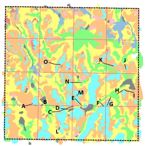
© Miriam Landa

2020

Small Rodent Winter Habitats in an Alpine Area, Finse, Norway

Miriam Landa

http://www.duo.uio.no/

Trykk: Reprosentralen, Universitetet i Oslo

II
Abstract
Small rodents in alpine areas are known to appear in multiannual cycles, usually with a
population peak every 3 – 5 years. Since the mid 1980’s, a dampening in these population
peaks have been observed in Northern Europe. Trying to understand the cause behind the
changes in population dynamics, a lot of different hypotheses have been put forward. One
hypothesis suggests that climate change is the main cause. As small rodents live under the
snowpack during winter, stable winter conditions are necessary for their survival. Changes in
winter climate may therefore affect small rodent survival. The aim is therefore to investigate
whether vegetation type and snow depth affects small rodents winter distribution in an alpine
area like Finse, Hardangervidda, in Norway. By gathering data on snow depth, vegetation
cover and winter activity of small rodents within a 1x1 km area, probability of rodent activity
could be estimated. Five out of six habitats were found to be suitable winter habitats for
rodents; snowbed, arctic-alpine heaths and leeside, boulder fields, open fen, and wet snowbed
and snowbed spring. Snow depth was shown to affect small rodent winter habitat preference
in snowbed habitats suggesting an optimum around two meters of snow. Similar peak patterns
could be argued found for both arctic-alpine heath and leeside and boulder fields however, the
uncertainties in the estimates were too large to conclude without further research.

                                                                                             III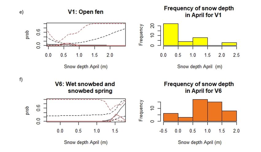
IV
Acknowledgement
To start off I want to thank my main supervisor Torbjørn H. Ergon and my co-supervisors
Simon Filhol, Anders Bryn and Stefaniya Kamenova. Thank you Torbjørn, for giving me the
opportunity to work on this project, for all the help and encouragement you have given me
throughout the whole project, and for all the feedback working on the manuscript. I am truly
thankful for all the insight and support. Simon, thank you so much for all the help you
provided in field, and for sharing your wide knowledge about snow and its properties. Anders,
thank you for all the help provided in field and with the manuscript. Thank you so much,
Stefaniya, for helping me with preparations regarding DNA analyses and for feedbacks
preparing me for the conference.

Thank you, to everyone in the GEco group and the LATICE group for sharing their
knowledge and making my fieldwork possible. Thanks to Finse Alpine Research Centre for
letting me stay there during my field work and for making my research possible by granting
me the Garpen stipend. Thanks to Anders Herland, for all the help you provided last summer
in field. I would also like to thank Sindre B. Jakobsen for all the fun weeks spent doing field
work at Finse, all the laughs and good help. To my friends and fellow office mates; thanks for
all the help and conversations. To my family; thanks for always believing in me and for
letting me choose my own path.

Lastly, a special thanks to Tor Arne Justad, thank you so much for all the support you have
provided during these last years. Thank you for all the help, encouragement and for all the
laughs. This experience would not have been the same without you.

                                                                                                  V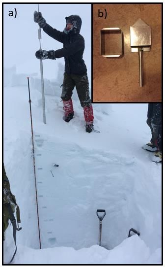
VI
Table of Contents
Abstract ................................................................................................................................ III
Acknowledgement ................................................................................................................. V
1      Introduction ....................................................................................................................1
2      Materials and Methods ....................................................................................................4
    2.1      Study Area ...............................................................................................................4
    2.2      Study species ............................................................................................................5
    2.3      Data gathering procedure..........................................................................................5
       2.3.1        Snow properties.................................................................................................6
       2.3.2        Snow depth measurements ................................................................................7
       2.3.3        Registration of rodent winter activity .................................................................8
    2.4      Data processing ........................................................................................................9
       2.4.1        DNA analysis on pellets ....................................................................................9
       2.4.2        Vegetation type classification ............................................................................9
       2.4.3        Snow depth measurements .............................................................................. 12
       2.4.4        Statistical analysis ........................................................................................... 12
       2.4.5        Hardness measurements .................................................................................. 13
3      Results .......................................................................................................................... 14
    3.1      Snow properties......................................................................................................14
       3.1.1        Snow hardness................................................................................................. 14
       3.1.2        Temperature loggers ........................................................................................ 14
    3.2      Rodent data ............................................................................................................ 17
       3.2.1        Probability of presence explained by vegetation type only ............................... 17
       3.2.2        Probability of presence when including snow depth as a predictor variable ......19
4      Discussion .................................................................................................................... 30
    4.1      Influence of vegetation type on small rodent winter habitats ................................... 30
    4.2      Influence of snow depth on small rodent winter habitats ......................................... 31
    4.3      Prospects and caveats ............................................................................................. 33
5      Conclusion .................................................................................................................... 35
References ............................................................................................................................ 36
Appendix A .......................................................................................................................... 42

                                                                                                                                       VII
VIII
1 Introduction
As key prey for a manifold of predators, rodents exhibit an important role for a wide range of
ecosystems (Kendall et al. 1998). Ranging from lowland to arctic environments, rodents like
lemmings and voles are revealed to affect the abundance of a variety of species (Elmhagen et
al. 2000, Côté et al. 2007, Ims and Fuglei 2005). Some predator species may persist regardless
of rodent abundance, while other might diverge as their prey of specialization disappear
(Elmhagen et al. 2000, Côté et al. 2007). Hence, a change in rodent population dynamics may
cause a diversity shift in ecosystems. Rodents are typically observed in cycles peaking every
3 – 5 years, however since the mid 1980’s, in Northern Europe, these high peaks have
dampened significantly (Elton 1924, Stenseth 1995, Ims et al. 2008, Cornulier et al. 2013,
Strann et al. 2002). The cause of the dampening is yet far from fully understood (Ims et al.
2008, Korslund and Steen 2006, Ims and Fuglei 2005, Cornulier et al. 2013, Hörnfeldt 2004,
Hörnfeldt et al. 2005, Kausrud et al. 2008). Although substantial research address different
drivers of rodent density cycles, most studies are carried out during the summer not winter
(Ims and Fuglei 2005, Korpimäki and Norrdahl 1998, Andersson and Jonasson 1986, Hanski
et al. 1991). Potential effects of winter conditions affecting rodents’ fitness might therefore
not be sufficiently explored. Due to this somewhat lacking insight on winter conditions and its
impact on rodent population dynamics, winter will be the main emphasis of this study.

Often rodent densities are associated with food availability, habitat conditions, physical
properties of snow and predation (Korslund and Steen 2006, Strann et al. 2002, Ims and
Fuglei 2005). Because small rodent spring densities largely affect the amplitude of the
population peak, winter survival is crucial (Cornulier et al. 2013). During winter and spring,
small rodents live under the snowpack. As a snowpack constantly change, the climatic
conditions during winter are important for rodent survival (Marchand 1996). At the bottom of
the snowpack a stable habitat is created; the subnivean space (Marchand 1996, Korslund and
Steen 2006). Here, rodents can forage and seek protection from both predators and the harsh
conditions above (Marchand 1996, Korslund and Steen 2006). The subnivean space is a brittle
and loosely arranged layer of snow crystals (typically faceted or depth hoar crystals) at the
bottom of the snowpack where it is easy for voles and lemmings to move around (Korslund
and Steen 2006, Marchand 1996, Fierz et al. 2009). This layer is created by physical gradients
of water vapor and temperature. When the depth of a snowpack reaches the hiemal threshold,
the threshold where insolating properties can be obtained, metamorphosis within the snow

                                                                                                  1
starts (Korslund and Steen 2006, Marchand 1996). Depending on other snow properties, the hiemal threshold usually forms when the snowpack reach 20 cm (Pruitt 1970). Heat is released from the soil into the snow, whereas wind and cold air cool the surface creating a gradient that is warm at the bottom and gradually cools towards the surface (Korslund and Steen 2006, Marchand 1996). This temperature gradient affects the level of water vapor within the snowpack. Water vapor travels from high densities to lower ones hence, creating an upward migration of water (Korslund and Steen 2006, Marchand 1996). In turn snow crystals at the bottom layer gets large and the bonds between them get weak, creating a perfect layer for small rodents to move around in (Korslund and Steen 2006, Marchand 1996). A dynamic snowpack is therefore essential for winter survival of small rodents. Different hypotheses have been suggested to explain the missing high peaks in rodent cycles (Hörnfeldt 2004). The hypothesis with best scientific support however, suggests that climate change during winter is what causes the observed damping of the density peaks (Cornulier et al. 2013, Hörnfeldt 2004, Hörnfeldt et al. 2005, Ims and Fuglei 2005, Ims et al. 2008, Kausrud et al. 2008, Korslund and Steen 2006). Climate change may alter rodent ecosystems directly by altering the snow properties. With changing winter climate, milder temperatures and rain on snow events becoming rapidly more frequent (Putkonen and Roe 2003, Peeters et al. 2018). With temperatures above the freezing point, water from the top layer of the snowpack or rain, will enter the snowpack and refreeze, creating ice layers (Marchand 1996). These ice layers can have a negative effect on rodents when freezing occurs close to the ground, restricting movement and inhibiting access to food. Additionally, freezing can act as a lid that traps gasses like CO2 and CH4 in the subnivean space, which in turn can have a negative effect on rodents trapped under the ice (Kausrud et al. 2008, Korslund and Steen 2006, Marchand 1996, Pirk et al. 2016). In addition to affect small rodents directly through changes in snow properties, climate change can affect small rodents by long term climate effects on their winter habitats by changing the vegetation structure (Myers-Smith et al. 2015, Myers- Smith et al. 2020). Increasing temperatures enhance shrub growth and expansion in alpine and arctic regions (Elmendorf et al. 2012, Tape et al. 2006). This can indirectly effect rodents in two ways: First, changing vegetation composition might alter food availability by outcompeting important food sources to rodents. Second, shrub expansion increase greening (Chapin et al. 2005). Greening affect climate by altering surface albedo, the fraction of sunlight reflected by the surface of Earth (Chapin et al. 2005). As a response to greening, surface albedo lowers, less radiation is reflected and in turn creating a positive feedback loop, 2
increasing temperature even more (Chapin et al. 2005, Barry and Chorley 2009). This can
have enormous effects on rodent food source and winter habitat.

At high-latitude alpine areas, such as Finse, Hardangervidda Norway, winters are long and
harsh. Snow typically starts accumulating from late September. As Finse has large micro-
topographic variations between different habitat types, snowmelt varies a lot. Snowmelt can
start early in April at ridges whereas boulder fields and snowbeds might not melt until July, or
not melt at all (personal communication with K. Aalstad, who estimated snowmelt-out day
maps for the study area at Finse using the method described in (Aalstad et al. 2020)). Small
rodents living here must therefore be highly adapted to these conditions to survive.

The lack of knowledge on how winter conditions may affect alpine and arctic ecosystems like
the one of small rodents is arguably of great interest. If rodents depend on stable winter
conditions to survive (and reproduce), human induced climate change might affect the
populations drastically. The aim of this master project is therefore, to study how vegetation
type and snow depth affect presence of rodents in an alpine region like Finse, which in turn
may be essential to increase the understanding of rodent cycles and their recent dampening.

                                                                                                3
2 Materials and Methods
2.1 Study Area
The study area is located at Finse,
northwestern part of Hardangervidda
mountain plateau, in south-central
Norway close to Finse Alpine
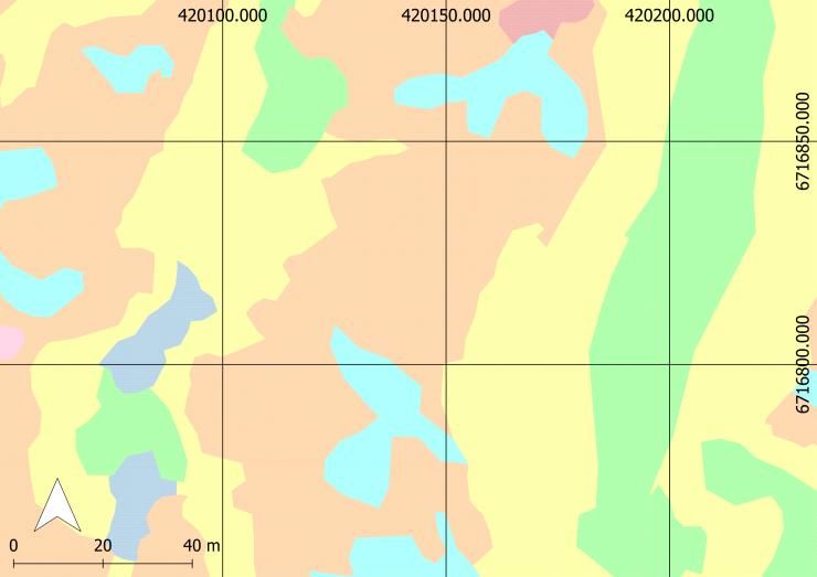
Research Centre (Fig. 1). Here, a
square of 11 km has been mapped
by the Department of Geoscience
(center coordinates 6716755N and
420058E in WGS84/UTM32N
Figure 1: Map displaying the study area at Finse, Hardangervidda
(ESPG:25832), 1200m a.s.l.). Since (pink square) and its location in Norway. Coordinates are provided
in WGS84, UTM32N (ESPG: 25832).
2011 the Land-Atmosphere
Interactions in Cold Environments
(LATICE) group have registered
snow property measurements like
depth and hardness in this area
(Gisnås et al. 2014). Additionally, a
group from the Natural History
Museum, Geo-Ecology research
group (GEco), has mapped the
vegetation within this area (Bryn
and Ullerud 2018). The study area
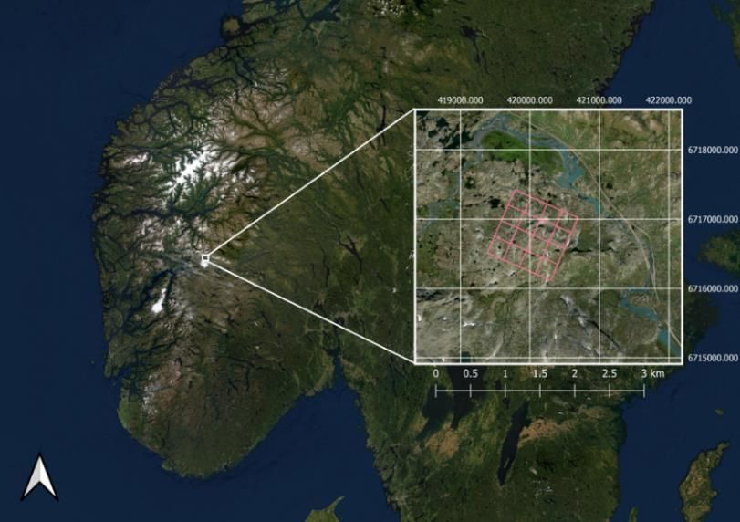
Figure 2: Vegetation map of a part of the study area. Different
covers a range of different
color codes represent the different vegetation types. Red: Bare
vegetation types common in alpine rock (T01); Orange: Arctic-alpine heaths and leesides (T3);
Yellow: Snowbeds (T07); Light blue: Exposed ridge (T14);
areas, covering the topographic- Green: Boulder fields (T27); Pink: Open fen (V1); Dark blue: Wet
ecological gradient from snowbeds snowbed and snowbed spring (V6). Coordinates are provided in
WGS84, UTM32N (ESPG: 25832).
to windswept ridges. Within these
gradients, micro-topography is very complex, creating a mosaic of micro-climates with
differences in e.g. terrain, wind, temperature and snow accumulation (Fig. 2) (Armbruster et
al. 2007). These small-scale differences can be of great importance for species composition
4(Armbruster et al. 2007). The area is located above the tree line and in the alpine vegetation
zone, in the slightly oceanic section (OC1) (Moen 1999). Vegetation like bilberry heath and
bryophytes are common (Moen 1999). The climate is cold, with an annual mean temperature
of -2.2°C measured at the closest weather station, Finsevatn (6718449N and 419320E in
WGS84/UTM32N (ESPG: 25832), 1210 m a.s.l.), and mean annual precipitation is 990mm
(1961-1990; www.eKlima.no).
2.2 Study species
There are five species small rodents at Finse belonging to three different genera: Lemmus,
Microtus and Myodes. Within the genus Microtus, there are two species, field vole (Microtus
agrestis) and tundra vole (Microtus oeconomus) respectively. Two species are represented
from Myodes, bank vole (Myodes glareolus) and grey red-backed vole (Myodes rufocanus).
From genus Lemmus the Norwegian lemming (Lemmus lemmus) is represented. They are all
herbivorous species with a diet of grasses, herbs and sedges (Microtus); grasses, mosses,
leaves and herbs (Myodes); or moss, sedges and grass (Lemmus) (Bjärvall 1997, Frislid 2004).
Voles and lemmings have an impressive rate of reproduction and a female can start mating at
only 16 days old (Ims and Fuglei 2005, Frislid 2004). Gestation is about 18 – 21 days and a
litter usually contains 5 – 7 young (Ims and Fuglei 2005, Frislid 2004). Additionally, a female
can start mating again only a few hours after giving birth, and in favorable years reproduction
might happen under the snowpack during winter (Ims and Fuglei 2005). Small rodents are of
high importance for the ecosystem especially in alpine regions were predators like the arctic
fox (Vulpes lagopus), weasel (Mustela nivalis) and snowy owl (Bubo scandiacus) depend on
the abundance of rodents for increased reproduction success (Ims and Fuglei 2005, Hörnfeldt
2004, Korpimäki and Krebs 1996).
2.3 Data gathering procedure
All measurements were done in 2019. Snow properties were sampled at two occasions, once
in beginning of March (3rd) and a second time in April (27th–29th). This ensures measurements
at different ages of the snowpack, giving a broader picture of the snow conditions for this
winter season. Density, hardness, depth, and temperature were measured using different
techniques (described below). Additionally, registration of signs of rodent winter activity was
carried out in a two-week period at the beginning of July. Here, the presence or absence of
5rodents was registered along transect lines crossing important topographic-ecological
gradients. Early snowmelt made one registration period sufficient.
2.3.1 Snow properties
Hardness measurement
The study design for measurements was based on variation in
vegetation types along the gradients ranging from ridge to
snowbed. Ensuring coverage of different elevation levels, habitats
and slope aspect within the area. The measurements were done
using a RAM-sonde which is a classical instrument to measure the
hardness of all the layers within a snowpack (Fig. 3 a) (Armbruster
et al. 2007). The instrument consists of a metal probe with a cone at
the bottom, and a weight hammer at the top. By dropping the
Figure 3: a) RAM-sonde
hammer from a certain height and measure the penetration depth of used to take hardness
measurements of a snow pit.
the probe, calculations can be made to describe the snow hardness
b) Boxed-shaped density
throughout the snowpack. cutter used for density
measurements (100 cm3).
Snow pits
Detailed stratigraphic measurements of the snowpack were done in snow pits from the top of
the snowpack to the ground. Measurements of total depth, temperature, and density every 5
cm were all taken for each snow pit. Density measurements were taken using a box-shaped
density cutter with known volume (100 cm3), then the snow from the cutter was weighted so
that density could be computed (Fig. 3 b) (Proksch et al. 2016). Additionally, hardness
measurements were taken (as described above) from the snow pits. The snow pit
measurements were used as complementary information for some of the hardness
measurements to help better understand the snowpack properties.
62.3.2 Snow depth measurements
Normal global position systems (GPS) have a
coordinate accuracy of about 2 – 3 m. For the
purpose of observing small rodents it was desirable to
improve the accuracy. Therefore, a differential GPS
(dGPS) was used, giving an accuracy of about +/- 25
cm. A reference dGPS station was set up, and then a
dGPS antenna was carried along the transect-lines in
an S-shape (Fig. 4). Resulting in accurate positioning Figure 4: Study area with red line indicating
the dGPS route.
of the snow depth measurements. dGPS
measurements were done once in March (3rd) and
once late in April (28th).
Additionally, drone photos collected
by the Department of Geoscience were
used to measure snow depth and
topography. During winter the drone
took geolocalized RGB (red, green,
blue) photographs of parts of the study
area. These photos were then set
together creating a “map” of the area
with some recovery where the photos
overlap. Then the photos were
processed through the
photogrammetric software MicMac Figure 5: The study area with the transect lines. A-O are the
small transects. The black dotted lines both mark the outer
following the procedure described by
lines of the 1x1 km area and four of the longer transect lines.
Girod and Filhol (Girod and Filhol in In addition, the pink lines mark six long transect lines within
the study area. Different color codes represent the different
press). Snow depth was calculated by vegetation types. Red: Bare rock (T01); Orange: Arctic-alpine
subtracting an aerial drone photo taken heaths and leesides (T3); Yellow: Snowbeds (T07); Light
blue: Exposed ridge (T14); Green: Boulder fields (T27); Pink:
in summer, from the winter photos Open fen (V1); Dark blue: Wet snowbed and snowbed spring
taken by the drone and calculate the (V6); Black: Limnic areas (L); White: Not classified.
height difference between the two. The
drone photos were taken at the beginning of March (1st) and late April (30th).
7Temperature loggers A 50-meter-long string with temperature sensors attached every 2 meters was placed along transect A (Fig. 5) in a terrain slope ranging from snowbed to ridge. The string was placed in early December (2018), as close to the ground as possible. This way, temperatures at the bottom of the snowpack (subnivean space) could be measured all winter. 2.3.3 Registration of rodent winter activity Shortly after snowmelt in July, fecal pellets were collected along transect lines to identify where the rodents lived during winter. Two different types of transects were used. The first type was set up by a master’s student at the Natural History Museum, Sindre B. Jakobsen, where he mapped the vegetation type and plant species composition in 1 m2 plots. In total 15 short transects were defined (A – O), ranging from 15 – 90 meters in length (Fig. 5). To ensure variation in both vegetation types and micro-topographic changes, all transects start at a ridge and end in a snowbed. The second type of transects were longer, around one kilometer long and 10 in total. Four of which mark the outer lines of the study area (Fig. 5: Black dotted square). Additional to the four outer transect lines, three horizontal and three vertical transects were placed within the outer ones with a distance of 250 meters between all of them (Fig. 5: Pink lines). Sampling method Rodent winter activity was recorded along all these transect lines. This was done by walking along the transect lines recording presence and absence at signs of winter activity by small rodents in every one-meter section, inspecting within a one-meter distance from the transect line on both sides. Presence of small rodents was recognized by fecal pellets, and only collected if it could be assumed to be fresh from the past winter. To identify if a pellet was fresh, signs of winter grazing, tunnels or nests had to be identified or the fecal pellet had to be wet and green/brown of color when crushed. All presences were marked on a GPS. Additionally, a position point was marked every 20 – 30 meters on the GPS to ensure distance. 8
From every section where presence of rodents was confirmed, at least 10 pellets were
gathered for DNA analysis. This was done using tweezers which were dipped in chlorine
between the different sample sites to prevent mixing of DNA. The pellets were put in teabags
and then into a zip-lock bag with silica gel to dry the pellets so that the bags could be stored.

2.4 Data processing

2.4.1 DNA analysis on pellets
Pellets gathered from sites where rodent activity was registered were dried and brought back
from the field. This was done so DNA analysis could be performed on each sample to get the
species. The samples were sent to Microsynth Ecogenics GmbH in Switzerland, for DNA
extraction by a polymerase chain reaction (PCR) method.

However, after running a pilot with 10 samples from the field, only 4 out of 10 samples were
identified to rodent species. This could imply that our samples are degraded or contaminated,
making it hard to distinguish species. Because the detection rate was so low, and time was
limited, the decision was to not go forward with the DNA analysis, only focusing on the
distribution of rodents in general.

2.4.2 Vegetation type classification
In field, rodent winter activity was registered on a one-meter scale. However, as registration
of every meter on a GPS would be too time consuming, GPS position were only marked at
signs of rodent winter activity and every 20 – 30 meters. Then data for absence points could
be added later using the statistical program R (version 3.6.1) (R Core Team 2019). To add the
missing absence points to get a one-meter scale, the GPS point had to be transformed from
latitude-longitude to UTM zone 32. This was done using the packages “rgdal” (version 1.4-7)
and “sp” (Bivand et al. 2019, Bivand et al. 2013b, Pebesma and Bivand 2005). Then one-
meter points could be added and projected onto a shapefile containing a map of the area by
using the additional package “raster” (Hijmans 2019). The same shapefile contained detailed
vegetation type information based on a mapping program organized by the Natural History
Museum in Oslo called Nature in Norway (NiN) (Bryn and Ullerud 2018, Bryn and Horvath

                                                                                                    9
in press). In total 10 864 one-meter sections were created, each section containing information about signs of rodent winter activity and vegetation type. Originally eight vegetation types were found however, limnic areas (L) and bare rock (T01) were taken out, leaving six types only (Table 1). Limnic areas were taken out simply because areas containing water was not searched, neither was it expected to find rodents in water. Areas of bare rock were taken out because they do not contain any vegetation and are therefore not a suitable habitat for rodents. Altogether leaving 10 432 one-meter sections with a vegetation type code and rodent winter activity information. All six vegetation types could further be classified into sub-levels depending on e.g. lime levels or water availability. However, these sublevels were not used in this project. 10
Table 1: Description of the different vegetation types (Halvorsen 2015, Bratli et al. 2019).

 Vegetation type          Vegetation name            Description                                                                        Number of one-
 code                                                                                                                                   meter sections
                                                                                                                                        (Percent
                                                                                                                                        coverage of total
                                                                                                                                        area (%))
 T03                      Arctic-alpine heath        Dwarf shrubs (Betula nana, Salix spp. and ericaceous species) and lichens          4074 (39.05)
                          and lee side               characterize the vegetation towards the ridges while herbs, graminoids and
                                                     bryophytes are typical of lee sides, which border on snowbeds.
 T07                      Snowbed                    Snowbeds are characterized by a combination of shortened growing seasons           2935 (28.14)
                                                     due to prolonged snow cover and, at the same time, shelter against low
                                                     temperatures and wind abrasion during winter. Vegetation cover vary at
                                                     different snow beds, some have no vegetation since snow do not melt every
                                                     year.
 T14                      Exposed ridge              Ecologically, this major type is characterized by lack of permanent snow           1756 (16.83)
                                                     cover in winter, periods with extremely low temperatures, freeze-drying
                                                     conditions and physical wind abrasion. Plants growing here are specialized,
                                                     stress-tolerant species dominated by lichens with scattered mosses and
                                                     vascular plants.
 T27                      Boulder field              Soil is lacking or sparsely present in “pockets” between boulders. Vegetation      1305 (12.51)
                                                     is typically restricted to saxicolous lichens and, eventually, mosses, or may be
                                                     absent.
 V1                       Open fen                   Peatforming Sphagnum species dominate the ground layer in lime-poor or             42 (0.40)
                                                     intermediately lime-rich fens while mosses other than Sphagnum (‘brown
                                                     mosses’) dominate in lime-rich fens.
 V6                       Wet snowbed and            Shortened growing season due to prolonged snow cover and influence by              320 (3.07)
                          snowbed spring             spring water.

                                                                                                                                                       11
2.4.3 Snow depth measurements Snow depth measurements using a dGPS were carried out both in March (26th) and April (28th). Due to some technical issues, data from the dGPS could only be obtained for March. In March the dGPS was carried as close to the transect lines as possible (Fig. 4). However, the distribution of snow made some areas inaccessible, resulting in few snow depth measurements (1364 one-meter sections out of 10 432 one-meter sections) close to the transect lines (85 hours) this approach had to be disregarded. Therefore, using the packages “spatialreg” and “spdep” a function which add 12
fictitious covariates as a predictor variable (based on Moran’s eigenvectors), removing the
autocorrelation from the residuals was added to a binomial GLM model (Bivand and Piras
2015, Bivand et al. 2013a, Bivand and Wong 2018). When fitting the model, sign of winter
activity was used as response variable with snow depth and vegetation type as additional
predictor variables to the new covariates. Both additive effects and interaction effects where
assessed in candidate models, and the effect of snow depth was explored with both linear and
quadratic models on the logit scale (Table 3, Table 4, and Table 5). To minimize the risk of an
over- or underfitted model, Akaike Information Criterion (AIC) was used to select the most
parsimonious model (Akaike 1974). AIC is used to predict the “out of sample” prediction
accuracy by evaluating the fit of the model to the data, then subtracting a penalty based on
number of parameters, minimizing the risk of under- or overfitting the model (Akaike 1974).
After choosing the best fitting model for each snow depth variable based on AIC, predictions
from these models were plotted to visualize rodent winter settlement in each habitat and at
different snow depths. Additionally, when a peak was found in snow depth the Delta Method
was used to calculate the peak and estimate the probability of rodent presence at the peak
(Cox 2005).
2.4.5 Hardness measurements
In total 31 different RAM-sonde measurements were done; 10 in March and 21 in April. Only
four vegetation types were included in the measurements (T03: Arctic-alpine heath and
leesides (n = 21), T07: Snowbed (n = 7), T14: Exposed ridges (n = 2) and V6: Wet snowbed
and snowbed spring (n = 1, hereafter called wet snowbed)). Hardness measurements
(including both RAM-sonde measurements and snow pits) were plotted and calculated using
an online software, niViz.org (www.niviz.org/). Additionally, the package “ggplot2” was used
to plot the difference in snow depth (Fig. 6) (Wickham 2016).
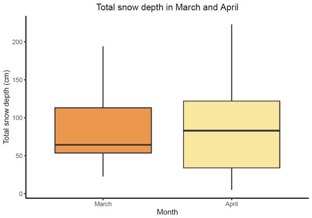
133 Results
3.1 Snow properties
Snow depth was measured in both March
and April. Not surprisingly, there was no
large change in snow depth between the two
months (Fig. 6).
3.1.1 Snow hardness
Figure 6: The dark orange box represents snow depth in
March; the yellow box represents snow depth in April.
In total, hardness was measured at 31 sites;
No significant change between snow depth in March and
10 in March and 21 in April. Indications snow depth in April (p-value = 0.98). Horizontal line
representing the median. Each box represents the 25th
towards harder snowpack in March were
and 75th percentile, with whiskers 1.5 times the
found, especially at 5 cm from the bottom interquartile range above 75th percentile and below 25th
percentile respectively.
(Fig. 7). Profiles of the individual hardness
measurements are found in the Appendix A.
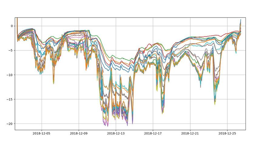
3.1.2 Temperature loggers
There was some variation in temperature
between the loggers, which could be due to
different snow coverage of individual loggers
(Fig. 8). However, no data on snow coverage
for each sensor was obtained. Comparing Figure 7: Figure shows mean hardness at 10 cm (left)
and 5 cm (right) above ground. The pink box represents
temperatures gathered from temperature hardness measures done in March; the green represents
loggers with air temperature from December April. See Fig. 6 for detailed explanation of the boxplot.
In the plot for hardness at 10 cm in March (left, pink
(www.eKlima.no, Fig. 9) it seems clear that box) two outliers are shown by two dots outside the
some of the loggers were covered boxplot.
sufficiently with snow as some loggers recorded temperatures much higher than the air
temperature. Some of the loggers only vary between -2 and -8 degrees Celsius, which is a lot
warmer than the air temperature. Others are just as cold at the air temperature indicating that
they were not fully covered by snow. This could be because they were placed at wind exposed
areas of the transect like at the top of the ridge. Altogether, the loggers show just how much
14variation in temperature there could be within just a few meters, visualizing the importance of
rodents choosing right habitats.
Additionally, the air temperature data from October to June help visualize just how much
variation in temperature there was during the winter season (Fig. 9). Until late November,
there were barely any days below 0 degrees. Then from the 19th of November to the end of
December a cooling period sets in. At the end of December and beginning of January there
were some days with temperatures above freezing. This happens again more frequently in
February with longer periods above freezing, then again in March. These kinds of shifts
between below and above freezing can cause melt-refreeze within a snowpack, which can
have damaging effects on the subnivean space (Marchand 1996). Additionally, by calculating
the mean temperature between 2002 – 2017, this winter season was somewhat special from
previous winter seasons. Mean air temperatures seem to be more extreme, having both colder
and warmer periods than usual, especially in early winter (Oct – Nov) and mid-winter (ending
of Jan – start of Feb, and March).
The temperature loggers within the snow were meant to operate all winter, but a fox bit over
the temperature cable at the end of December. Therefore, temperature measures were only
obtained for a few weeks.
15Figure 8: Temperature from the temperature loggers. The different colors represent unique loggers within the long line of loggers. The x-axis showing time (year-month-day), the y-axis shows temperature (°C). The different loggers show that there is some variation between the loggers. Some of the variation can probably be explained by amount of snow coverage. Figure 9: Air temperatures from October 2018 to July 2019. Red line: Mean daily temperature; Blue line: Maximum daily temperature; Orange line: Minimum daily temperature; Black line: Mean winter temperature calculated from winter temperatures between 2002 – 2017. Data gathered from a weather station right next to Finse Alpine Research Station which is close to the study area (6718447N and 419320E, WGS84, UTM32N (ESPG: 25832), 1210 m a.s.l.) and obtained from www.eKlima.no. 16
3.2 Rodent data

3.2.1 Probability of presence explained by vegetation type only
The binomial generalized linear model with presence/absence of pellets as a binary response
and only vegetation type as predictor variable, estimated the probability of rodent winter
activity for each of the habitats (Table 2). The results show that small rodents are present in
all habitats however, as exposed ridge (T14) have such low probabilities (0.2 – 0.7%, 95%
confidence interval) it might be reasonable to assume that rodents do not live here, and that
the presence found might be false positives (pellets from previous summers or after
snowmelt). Which one of the habitats that are most likely to occupy small rodents during
winter is somewhat unclear, as open fen (V1), wet snowbed (V6), and snowbed (T07) all have
overlapping confidence intervals (Table 2). The uncertainties found for wet snowbed (1.3 –
4.7%, 95% confidence interval), and open fen (0.5 – 6.5%, 95% confidence interval) might be
explained as these habitats are not very common in the study area (3.07% and 0.4%
coverage). It seems that small rodents are slightly more likely to occupy snowbed habitats
(2.8 – 4.1%, 95% confidence interval) than both arctic-alpine heath and leeside (1.4 – 2.1%,
95% confidence interval), and boulder field (1.4 – 3.0%, 95% confidence interval) as the
confidence interval barely overlap with the two others.

                                                                                                  17
Table 2: The probability of small rodents occupying the different habitat types during winter. Standard error and
upper and lower 95% confidence interval are included. The last column show percent coverage of each
vegetation type within the study area.
Vegetation type Probability of Lower Upper Percent
presence at confidence confidence coverage of
vegetation type interval interval total area (%)
T03: Heath and 0.017 0.014 0.021 39.05
lee side
T07: Snowbed 0.034 0.028 0.041 28.14
T14: Exposed 0.004 0.002 0.007 16.83
ridge
T27: Boulder 0.020 0.014 0.030 12.51
fields
V1: Open fen 0.018 0.005 0.065 0.40
V6: Wet 0.025 0.013 0.047 3.07
snowbed and
snowbed spring
183.2.2 Probability of presence when including snow depth as a
predictor variable
Table 3 (a, b, and c) display the different candidate models for the different snow depth
variables (dGPS and drone for March, and drone for April).
Table 3: Candidate models with a) snow depth measured in March (dGPS) as a predictor variable, b) snow
depth measured in March (drone) as a predictor variable, and c) snow depth measured in April (drone) as a
predictor variable. “Pellet” represents the binary response variable indicating whether signs of rodent winter
activity were found, and "Veg" represents the predictor variable with different vegetation types. The predictor
variable with the different snow depth measurements is represented by a) "SD_dGPS", b) "SD_March", and c)
"SD_April". The sample size was a) n = 1364, b) n = 3006, and c) n = 5801. All tables are sorted by increasing
AIC values. *Model chosen as best fitting the data by AIC score. **Model for linear/quadratic comparison.
a)
Candidate models for snow depth in March (dGPS) AIC
Pellet ~ Veg + SD_dGPS + SD_dGPS2 333.16*
Pellet ~ Veg + SD_dGPS 336.41**
Pellet ~ Veg + SD_dGPS + Veg : SD_dGPS 338.52
Pellet ~ Veg + SD_dGPS + SD_dGPS2 + Veg : SD_dGPS + Veg : SD_dGPS2 344.78
b)
Candidate models for snow depth in March (drone) AIC
Pellet ~ Veg + SD_March + Veg : SD_March 766.97*
Pellet ~ Veg + SD_March 770.23
Pellet ~ Veg + SD_March + SD_March2 785.93
Pellet ~ Veg + SD_March + SD_March2 + Veg : SD_March + Veg : 788.70**
SD_March2
c)
Candidate models for snow depth in April (drone) AIC
Pellet ~ Veg + SD_April + SD_April2 + Veg : SD_April + Veg : SD_April2 1507.40*
Pellet ~ Veg + SD_April + SD_April2 1509.00
Pellet ~ Veg + SD_April + Veg : SD_April 1520.50**
Pellet ~ Veg + SD_April 1530.50
19For measurements done in March, both dGPS and drone, some of the vegetation types did not have any presence points and are therefore not included in Figure 10 and Figure 11. Figure 10: The probability of rodent presence at different snow depths in March (measured with dGPS) (left), plotted with habitat specific linear effects (black line) and 95% confidence interval (black dotted lines), and the habitat specific quadratic effects (red line) and 95% confidence interval (red dotted lines). Each vegetation type has a histogram visualizing the frequency of each snow depth (right). Some have snow depths lower than 0, this is due to measurement error introduced when comparing the orthographic projection and the winter images. Because some of the vegetation types did not have any presence point the model could not estimate the probability. Therefore, only two out of six vegetation types are represented here: a) T03: Arctic-alpine heath and leesides; b) T07: Snowbed. 20
Table 4: Mean snow depth and snow depth at peak of probability for the different vegetation types measured in March with a dGPS. 95% confidence intervals are written in
brackets after “probability of presence at mean snow depth”, “snow depth at peak of probability of presence” and “probability of presence at peak”. The cover percentage of
each vegetation type is calculated based on sample size for the individual vegetation types and total subset sample size (n = 1364). Model 1 indicate the habitat specific
linear effects model (1), and model 2 indicate the habitat specific quadratic effects. All snow depths are in meters.

 Model Vegetation type             Mean snow            Probability of             Snow depth at peak                 Probability of          Sample size for each
                                   depth March          presence at mean           probability of presence            presence at             vegetation type
                                   (m)                  snow depth                 (m) (Confidence interval           peak                    (Percent coverage
                                   (Standard            (Confidence                (m))                               (Confidence             (%))
                                   error (m))           interval)                                                     interval)
 1          T03: Arctic-           1.16 (0.29)          0.016 (0.009, 0.028)                                                                  650 (47.65)
            alpine heath and                                                                       -                            -
            leeside
 1          T07: Snowbed           2.30 (0.30)          0.030 (0.017, 0.053)                       -                            -             385 (28.23)

 2          T03: Arctic-           1.16 (0.45)          0.016 (0.007, 0.037) 1.62 (0.71, 2.52)                        0.017, (0.006           650 (47.65)
            alpine heath and                                                                                          0.045)
            leeside
 2          T07: Snowbed           2.30 (0.49)          0.028 (0.010, 0.071) 1.62 (0.71, 2.52)                        0.031 (0.013,           385 (28.23)
                                                                                                                      0.073)

                                                                                                                                                                        21
22
Figure 11: The probability of rodent presence at different snow depths in March (measured with drone) (left),
plotted with habitat specific linear effects (black line) and 95% confidence interval (black dotted lines), and the
habitat specific quadratic effects (red line) and 95% confidence interval (red dotted lines). Each vegetation type
has a histogram visualizing the frequency of each snow depth (right). Some have snow depths lower than 0, this
is due to measurement error introduced when comparing the orthographic projection and the winter images.
Because some of the vegetation types did not have any presence point the model could not estimate the
probability. Therefore, only four out of six vegetation types are represented: a) T03: Arctic-alpine heath and
leesides; b) T07: Snowbed; c) T27: Boulder fields; d) V6: Wet snowbed and snowbed spring.

                                                                                                                 23
Table 5: Mean snow depth and snow depth at peak of probability for the different vegetation types measured in March with a drone. 95% confidence intervals are written in
brackets after “probability of presence at mean snow depth”, “snow depth at peak of probability of presence” and “probability of presence at peak”. The cover percentage of
each vegetation type is calculated based on sample size for the individual vegetation types and total subset sample size (n = 3006). Model 1 indicate the habitat specific
linear effects model (1), and model 2 indicate the habitat specific quadratic effects. All snow depths are in meters.
Model Vegetation Mean snow depth Probability of Snow depth at peak Probability of Sample size for
type March (m) presence at mean probability of presence presence at peak each vegetation
(Standard error snow depth (m) (Confidence (Confidence type (Percent
(m)) interval (m)) interval) coverage (%))
1 T03: Arctic- 0.65 (0.22) 0.015 (0.010, 1168 (38.86)
alpine heath and 0.023) - -
leeside
1 T07: Snowbed 1.28 (0.18) 0.043 (0.031, - - 839 (27.91)
0.061)
1 T27: Boulder 1.48 (0.42) 0.006 (0.002, - - 740 (24.62)
field 0.013)
1 V6: Wet 1.41 (0.42) 0.123 (0.057, 87 (2.89)
snowbed and 0.245) - -
snowbed spring
2 T03: Arctic- 0.65 (0.26) 0.015 (0.009, 1168 (38.86)
alpine heath and 0.025) - -
leeside
2 T07: Snowbed 1.28 (0.18) 0.073 (0.052, 2.36 (1.87, 2.85) 0.128 (0.085, 0.189) 839 (27.91)
0.102)
2 T27: Boulder 1.48 (0.40) 0.009 (0.004, - - 740 (24.62)
field 0.021)
2 V6: Wet 1.41 (0.46) 0.099 (0.042, 87 (2.89)
snowbed and 0.216) - -
snowbed spring
2425
Figure 12: The probability of rodent presence at different snow depths in April (measured with drone) (left),
plotted with habitat specific linear effects (black line) and 95% confidence interval (black dotted lines), and the
habitat specific quadratic effects (red line) and 95% confidence interval (red dotted lines). Each vegetation type
has a histogram visualizing the frequency of each snow depth (right). Some have snow depths lower than 0, this
is due to measurement error introduced when comparing the orthographic projection and the winter images. All
six vegetation types are represented: a) T03: Arctic-alpine heath and leesides; b) T07: Snowbed; c) T14: Exposed
ridges, d) T27: Boulder fields; e) V1: Open fen; V6: Wet snowbed and snowbed spring.

26
Table 6: Mean snow depth and snow depth at peak of probability for the different vegetation types measured in April with a drone. 95% confidence intervals are written in
brackets after “probability of presence at mean snow depth”, “snow depth at peak of probability of presence” and “probability of presence at peak”. The cover percentage of
each vegetation type is calculated based on sample size for the individual vegetation types and total subset sample size (n = 5801). Model 1 indicate the habitat specific
linear effects model (1), and model 2 indicate the habitat specific quadratic effects. All snow depths are in meters.

 Model Vegetation type                  Mean snow            Probability of                Snow depth at peak          Probability of              Sample size for
                                        depth April          presence at mean              probability of              presence at peak            each vegetation
                                        (m) (Standard        snow depth                    presence (m)                (Confidence                 type (Total
                                        error (m))                                         (Confidence                 interval)                   sample size (%))
                                                                                           interval (m))
 1          T03: Arctic-alpine          0.31 (0.17)          0.017 (0.012, 0.024)                    -                             -               2086 (35.96)
            heath and lee side
 1          T07: Snowbeds               1.57 (0.13)          0.045 (0.035, 0.058)                      -                           -               1573 (27.12)
 1          T14: Exposed ridge          0.00 (0.39)          0.006 (0.003, 0.012)                      -                           -               1167 (20.12)
 1          T27: Boulder fields         2.02 (0.26)          0.013 (0.008, 0.022)                      -                           -               889 (15.32)
 1          V1: Open fen                0.68 (0.73)          0.023 (0.005, 0.091)                      -                           -               37 (0.64)
 1          V6: Wet snowbed             0.91 (3.15)          0.001 (0.000, 0.286)                      -                           -               49 (0.84)
            and snowbed spring
 2          T03: Arctic-alpine          0.31 (0.18)          0.021 (0.015, 0.029)                      -                           -               2086 (35.96)
            heath and lee side
 2          T07: Snowbeds               1.57 (0.16)          0.056 (0.042, 0.075)          2.04 (1.62, 2.46)           0.059 (0.043, 0.081)        1573 (27.12)

 2          T14: Exposed ridge          0.00 (0.41)          0.005 (0.002, 0.012)                      -                         -                 1167 (20.12)
 2          T27: Boulder fields         2.02 (0.35)          0.020 (0.010, 0.040)          2.22 (1.69, 2.75)           0.021 (0.010, 0.042)        889 (15.32)

 2          V1: Open fen                0.68 (1.22)          0.086 (0.008, 0.518)                      -                           -               37 (0.64)
 2          V6: Wet snowbed             0.91 (28.89)         0.000 (0.000, 1.000)                      -                           -               49 (0.84)
            and snowbed spring

                                                                                                                                                                        27
The variation seen within one vegetation type between the different snow depth variables, e.g. boulder field (Fig. 11 c and Fig. 12 d), arise as each snow depth variable has an individual subsample of the whole dataset (dGPS March n = 1364, drone March n = 3006, and drone April = 5801, total sample size N = 10 432). Arctic-alpine heath and leeside (T03) show different patterns in the different snow depth variables. For the snow depth variable from March using drone, rodents are found, but there seem to be no preference towards snow depths, at least not between 0 – 2 meters where the sample size is largest (Fig. 11 a). The two other snow depth variables however seem to indicate an effect of snow depth. The snow depth variable from March using dGPS indicates a preference in snow depth of around 1.62 meters (Fig. 10). The confidence interval on the other hand is very large, ranging from 0.7 – 2.5 meters, making the uncertainties related to where the peak will form large (Fig. 10 a). The snow depth variable from April using drone show a slight increase in preference towards higher snow depths, although after 1.5 meters of snow the uncertainties become larger as the sample size decreases (Fig. 12 a). Even though the three different snow depth variables show varying degree in whether snow depth will affect small rodents’ winter habitat choice, they all indicate that small rodents occur in arctic- alpine heath and leeside. In snowbed habitats (T07) there seem to be an optimal snow depth as rodents seem to occupy snowbed habitats with around 2 meters of snow more frequently than at other snow depths (1.62 m, 2.02 m and 2.36 m respectively). Even though there is variation in confidence intervals between the where the peak in snow depth will form (0.71 – 2.52 m, 1.87 – 2.85 m, and 1.62 – 2.46 m, 95% confidence interval) and the probability of rodent occupancy (1.3 – 7.3%, 8.5 – 18.9%, and 4.3 – 8.1%, 95% confidence interval), they all suggest a preference towards snow depths of around 2 meters. In contrast to snowbeds, where all the snow depth variables suggest the same pattern, the two different snow depth variables for boulder field (T27) show two completely different patterns. Here the snow depth variable from March using drone (Fig. 11 c) suggest that rodents are not present at all, whilst the snow depth variable from April using drone (Fig. 12 d) suggest that there is a peak in preference towards 2.22 meters of snow. As the model only accounting for vegetation type both have larger sample size and suggest rodent presence in boulder field habitats (Table 2), it seems unlikely that the snow depth variable from March (drone) would be the true distribution of small rodents during winter (Fig. 11 c). 28
As suggested for the model only accounting for vegetation type (Table 2), rodents seem to not
be present at exposed ridge (T14), suggesting that this type of habitat is not suited for rodents
during winter (Fig. 12 c). For both wet snowbeds (V6), and open fen (V1) the uncertainties
related to the snow depth variables are too large that no inference can be made in this study
regarding the effect snow depth might have on small rodent winter habitat choice (Fig. 12 e, f
and Fig. 11 d).

                                                                                                29
4 Discussion The aim of this study was to gain more information about how vegetation type and snow depth affect small rodents winter distribution in an alpine area. This was done by measuring both snow depth and vegetation type in a 1x1 km area at Finse, Norway, and gathering data on signs of winter activity after snowmelt. The probability of rodent settlement in different habitats and at different snow depths could then be estimated. Snow conditions the year of the study was somewhat unusual with less snow cover than normal and melting happening earlier than usual. Additionally, small rodent winter density was very low, making it harder to estimate preference for the different habitats and snow depths. As more rodent presence data would give better estimates with less uncertainties in the models it could be argued that these kinds of studies should be performed in peak years only. On the other hand, studies have found that habitats get saturated in years of high small rodent densities, forcing small rodents to occupy habitats that they usually would not occupy (Hansson 1979, Löfgren 1995). Measuring density peak-years might therefore create an inaccurate description of habitat preference. The findings of this study are therefore only representable in years with low population densities. 4.1 Influence of vegetation type on small rodent winter habitats Small rodents seemed to prefer five out of six habitats included in this study. Wet snowbed, open fen, snowbed, arctic-alpine heath and leeside, and boulder fields all have relatively high probability (1.3 – 4.7%, 0.5 – 6.5%, 2.8 – 4.1%, 1.4 – 2.1% and 1.4 – 3% respectively) of being occupied by rodents during winter without large uncertainties. As both graminoids and bryophytes are abundant in snowbeds, open fen, and heaths and leesides, the preference found towards these areas might be explained as they serve as suitable food source to rodents (Bratli et al. 2019, Bjärvall 1997, Frislid 2004). Wet snowbed and boulder fields, on the other hand, have little to no vegetation cover hence food availability might not be the only factor explaining rodent presence (Bratli et al. 2019). It has been suggested that plant composition in itself is not the only factor determining rodent winter habitat, rather snow conditions and micro-topography might be the important factors (Reid et al. 2012). 30
In contrast to boulder field, snowbed, open fen, wet snowbed, and arctic-alpine heath and
leeside, where rodents were found to be abundant, rodents were barely found at all at exposed
ridges (0.4 – 0.7%, 95% confidence interval). This might not be surprising as exposed ridges
are classified as unstable during winters as little vegetation thrive here (Bratli et al. 2019). As
only visual ques were used when sampling rodent presence data, there will be a risk of
sampling pellets from previous years or from the following spring (after snowmelt), which
can create false presence points in the data. This might explain why some presence points was
found at exposed ridges even as the habitat seems unsuitable during winter. Altogether these
result show that there is a preference in winter habitat.

4.2 Influence of snow depth on small rodent winter
habitats
Winter conditions like snow depth and snow hardness have been found to affect rodent
settlement and densities (Kausrud et al. 2008, Korslund and Steen 2006). As the hiemal
threshold, the threshold where insolating properties can be obtained, is usually reached at 20 –
60 cm of snow, it is reasonable to assume that snow depth alter rodent habitat selection (Reid
et al. 2012, Duchesne et al. 2011, Marchand 1996). When the hiemal threshold is not reached,
the subnivean space cannot form making it hard for small rodents to move and forage during
winter (Korslund and Steen 2006, Marchand 1996). From the results, the mean snow depth in
areas of exposed ridge were estimated to 0 meters, with barely any samples with more than
0.4 meters of snow. This makes exposed ridge an unsuitable habitat both in terms of food
availability (provided by vegetation type) and in terms of insulation and protection (snow
depth).

Yet, snow depth and the hiemal threshold are not the only factors that can alter snow
properties, air temperature has been found to be a highly significant predictor of both snow
hardness and duration of snow cover (Kausrud et al. 2008). As air temperature above freezing
happened at several occasions during winter, melt-refreeze or rain on snow events could be
expected, hence might explain both the hard, icy layers found at the bottom of the snowpack
in both March and in April, and the unusual early melt (Putkonen and Roe 2003, Marchand
1996, Peeters et al. 2018, Kausrud et al. 2008). It could therefore be argued that the winter
conditions that year was somewhat suboptimal to a small rodent. Additionally, the results and
personal observations done in field, suggest low densities in small rodent populations both in

                                                                                                 31
winter and in spring (only one rodent was observed for the whole spring and summer). This is as predicted since suboptimal winter conditions can have a great impact on small rodent spring density (Kausrud et al. 2008). At Finse, some snowbeds are so deep that they do not fully melt during summer. Beneath a snowpack that does not melt, no vegetation would thrive hence making it an unsuitable habitat for rodents (Korslund and Steen 2006). Other snowbed areas have less snow that do melt during summer. As supported by previous research, snowbeds were found to be a suitable winter habitat for rodents in all three snow depth variables, and snow depth were shown to have an effect on habitat suitability (Moen et al. 1993, Reid et al. 2012). Interestingly, there seem to be a peak in probability of rodents occupying snowbed habitats around two meters (+/- 40 cm between the three different snow depth variables) suggesting that there is an optimal snow depth for rodents when choosing winter habitat. This type of optimum might reflect the threshold between areas of snowbeds that melt late in the summer and that do not melt at all, hence have no food available for rodents (Halvorsen 2015). Another explanation is that the optimum could be a result of predation. A study conducted in Sweden tested whether snow depth affected rodent consumption in red foxes (Vulpes vulpes) (Lindström and Hörnfeldt 1994). The result was a negative correlation between consumed small rodents and snow depth, with a maximum snow depth measurement of 1.20 meters (Lindström and Hörnfeldt 1994). Consequently, the two meters optimum seen in the data might be a response to predation, were predators struggle to access small rodents hence increasing small rodents’ winter survival. Although dwarf shrub heaths have been suggested as a preferable small rodent winter habitat, snow depth was not found to have an effect on rodents living in arctic-alpine heath and leeside (Moen et al. 1993). It could be argued that the snow depth variable from March using a dGPS indicate a peak however, both the uncertainties to where the peak will form (0.7 – 2.5 meters) and the uncertainties regarding the probability of a rodent occupying the habitat (0.6 – 7.3%, 95% confidence interval) are so large that snow depth cannot be concluded to affect small rodents habitat choice. The model with the snow depth variable from April using a drone, suggests an increasing probability of rodent presence as snow depth increases. The increasing pattern forms as the sample size gets smaller, hence suggesting that small rodents live here, but that the data cannot predict how snow depth affect the small rodents’ winter habitat choice. It could be that with higher rodent population densities, the peak would be 32
You can also read