Errors in top-down estimates of emissions using a known source
←
→
Page content transcription
If your browser does not render page correctly, please read the page content below
Atmos. Chem. Phys., 20, 11855–11868, 2020
https://doi.org/10.5194/acp-20-11855-2020
© Author(s) 2020. This work is distributed under
the Creative Commons Attribution 4.0 License.

Errors in top-down estimates of emissions using a known source
Wayne M. Angevine1,2 , Jeff Peischl1,2 , Alice Crawford3 , Christopher P. Loughner3,4 , Ilana B. Pollack5 , and
Chelsea R. Thompson1,2
1 Cooperative Institute for Research in Environmental Sciences (CIRES), University of Colorado, Boulder, Colorado, USA
2 NOAA  Chemical Sciences Laboratory, Boulder, Colorado USA
3 Atmospheric Sciences Modeling Division, Air Resources Laboratory, NOAA, College Park, MD, USA
4 Cooperative Institute for Satellite Earth System Studies (CISESS)/Earth System Science Interdisciplinary Center (ESSIC),

University of Maryland, College Park, MD, USA
5 Department of Atmospheric Science, Colorado State University, Ft. Collins, Colorado USA

Correspondence: Wayne M. Angevine (wayne.m.angevine@noaa.gov)

Received: 20 February 2020 – Discussion started: 21 April 2020
Revised: 21 August 2020 – Accepted: 1 September 2020 – Published: 22 October 2020

Abstract. Air pollutant emissions estimates by top-down           data with emissions factors, essentially counting sources and
methods are subject to a variety of errors and uncertainties.     multiplying by their individual emissions. This is the main
This work uses a known source, a coal-fired power plant,          method used to produce official inventories. Top-down meth-
to explore those errors. The known emissions amount and           ods use measurements of atmospheric concentrations to es-
location remove two major types of error, facilitating un-        timate emissions. Both types of methods are subject to sub-
derstanding of other types. Biases and random errors are          stantial uncertainty and often disagree (e.g., Hsu et al., 2010).
distinguished. A Lagrangian dispersion model (HYSPLIT)               The main purpose of this work is to evaluate some of the
is run forward in time from the known source, and virtual         errors and uncertainties in top-down methods while control-
measurements of the resulting tracer plume are compared to        ling other sources of uncertainty. Evaluating the errors and
actual measurements from research aircraft. Four flights in       uncertainties of top-down methods is difficult. Not only the
different years are used to illustrate a variety of conditions.   emissions amounts but their location, distribution, and timing
The measurements are analyzed by a mass-balance method,           are often unknown. Attempts to constrain all these matters
and the assumptions of that method are discussed. Some of         simultaneously result in grossly under-determined systems.
those assumptions can be relaxed in analysis of the mod-          Most often the under-determination is dealt with by employ-
eled plume, allowing testing of their validity. Meteorological    ing Bayesian statistical methods, which introduce further er-
fields to drive HYSPLIT are provided by the European Cen-         rors and uncertainties and remove the desired independence
tre for Medium-Range Weather Forecasts Fifth Reanalysis           of the top-down and bottom-up methods.
(ERA5). A unique feature of this work is the use of an en-           In this work, we start with an emission source known
semble of meteorological fields intrinsic to ERA5. This anal-     in quantity, timing, and location. That source is the Mar-
ysis supports reasonably large (30 %–40 %) uncertainties on       tin Lake coal-fired power plant in eastern Texas. It is lo-
top-down analyses.                                                cated in reasonably simple, flat terrain. Stack emissions of
                                                                  several gasses are measured by continuous emissions moni-
                                                                  toring systems (CEMSs). Concentration measurements from
                                                                  aircraft are used to estimate emissions by mass balance and
1   Introduction                                                  to compare with modeled concentrations. Here we use sul-
                                                                  fur dioxide (SO2 ), nitrogen oxides (NOy ), and carbon diox-
Emissions of air pollutants must be known for modeling            ide (CO2 ). SO2 is emphasized because its peak concentra-
of exposure and planning for compliance with concentra-           tion measured in aircraft traverses is well defined above the
tion standards. Bottom-up and top-down methods are used           regional background. SO2 is lost to surfaces and converted
to estimate emissions. Bottom-up methods combine activity

Published by Copernicus Publications on behalf of the European Geosciences Union.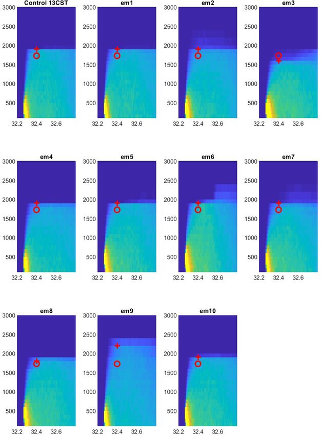
11856                                                      W. M. Angevine et al.: Errors in top-down estimates of emissions

to sulfate aerosol, but that conversion is slow compared to       of bias. So is the difference between an ensemble mean re-
the transport time of the main transects we use here, which       sult and reality. The statistics of differences between results
are usually 30–60 min downwind of the stack. CEMS data            from all ensemble members are estimates of random uncer-
are also uncertain, but we assume that those uncertainties        tainty. The quality of these estimates depends on the design
are small, i.e., < 10 % (Peischl et al., 2010), relative to the   and quality of the ensemble.
other uncertainties treated here. For the purposes of this pa-       Meteorological quantities have been identified as major
per, CEMS data are considered the “reality” with which other      sources of error and uncertainty in emissions estimates.
estimates are compared.                                           These can be divided into several classes. Wind direction er-
   Emissions can be estimated from observations alone under       rors displace the plume (or the source in an inverse analysis).
certain non-trivial assumptions. Inverse modeling is used to      Wind speed errors change the magnitude of the plume and
allow relaxation of some of those assumptions. In this work,      its timing with respect to time-varying emissions. Mistaken
we replace some of the observations with (forward) modeled        diagnosis of the mixing height affects the concentrations and
values, in varying combinations. This allows us to character-     may contribute to violation of the well-mixed assumption.
ize and estimate errors arising from the models, and it is a      Errors in the transport model are also important. Under- or
step toward understanding errors and uncertainties in inverse     over-estimation of horizontal dispersion changes the plume
modeling.                                                         width. Discretization in either horizontal or vertical dimen-
   We attempt to distinguish between error and uncertainty        sions may add noise or uncertainty. Physical situations that
within this work. Error is the difference between an ana-         are correctly handled in the models may still lead to errors
lyzed value and the true value, in this case, of the emission     in some analyses. For example, temporal variation (unsteadi-
rate. Uncertainty is an estimate of the error that we expect      ness) of wind can result in storage of pollutant that violates
in the absence of knowledge of the truth (Joint Committee         the assumption of steady wind in mass balance analysis. This
for Guides in Metrology, 2008). Error and uncertainty have        can be exacerbated if the winds are not updated often enough
systematic and random components. Systematic error is syn-        in the transport model.
onymous with bias, that is, persistent differences of one sign
between reality and a result of analysis. The distinction is
neither precise nor crisp, and terms are not always used care-    2   Data
fully. Atmospheric measurements rarely have enough sam-
ples to reliably distinguish the two. Bias can be introduced      The Martin Lake power plant complex is located in fairly
by the use of methods or assumptions that most often move         simple terrain in eastern Texas (32.260◦ N, 94.570◦ W). It has
the result in one direction. For example, a low bias in a wind    three stacks that are each 452 ft (138 m) high. The stacks are
speed measurement will result in a low bias in the emissions      spaced 100 m apart.
estimated by mass balance. Random differences have many              The measurements used here were taken by NOAA scien-
possible causes, one important cause being sampling uncer-        tists aboard NOAA or NCAR research aircraft. Flights down-
tainty, that is, the difference between the mean of a quantity    wind of the Martin Lake power plant were made in four years
measured with a small number of samples and the true (en-         (2000, 2006, 2013, and 2015). Dates are shown in Table 1.
semble) mean (Wilks, 2011). The distinction is important for      The flights were planned to intercept the plume at least once
several reasons. Reporting a small uncertainty with possibly      and usually several times. Downwind distances were chosen
large unknown biases can lead to incorrect policy decisions.      to satisfy the conditions for mass balance analysis (see be-
Bayesian analyses assume that the measurements and prior          low), far enough downwind for the plume to be well mixed
have zero mean error and (usually) Gaussian uncertainty, and      through the boundary layer in the vertical but close enough
the proper characterization of the error covariances is criti-    for the concentration signal to be strong and to minimize
cal to a good result. From a practical point of view, repeated    chemical transformations.
measurements can reduce random uncertainty but cannot re-            For all four flights, SO2 was measured using a modified,
duce bias.                                                        commercial, pulsed UV fluorescence instrument, a Thermo
   Errors and uncertainties in the meteorological fields (mod-    Environmental Instruments, Inc., model 43S (Ryerson et al.,
eled or measured) used in analyses propagate directly into the    1998). The 1 Hz measurements have an estimated 1σ preci-
result. Since we only measure one realization of the chaotic      sion of ±0.3–1 ppbv and a 1σ uncertainty of ±10 %–12 %,
atmosphere, we never have an ensemble average (statistically      depending on year. NOy was measured by chemilumines-
speaking). Normally, only a single meteorological field is        cence after conversion to NO in a heated gold catalyst (Ry-
used. The numerical weather prediction community has been         erson et al., 1999). The 1 Hz precision ranged from 0.015 to
moving steadily toward producing ensemble output, that is,        0.4 ppbv, and uncertainty ranged from ±10 % to 12 %, de-
well-designed sets of multiple realizations (Palmer, 2018).       pending on year. CO2 was measured by infrared absorption
These can provide a rough method to distinguish between           using a LI-COR 6262 in 2000 and 2006 (Peischl et al., 2010),
bias and random uncertainty. The difference between the re-       and a Picarro 1301-m in 2013 and 2015 (Peischl et al., 2012).
sult produced from a control run and reality is an estimate       The 1 Hz precision was at or below ±0.1 ppm for all flight

Atmos. Chem. Phys., 20, 11855–11868, 2020                                         https://doi.org/10.5194/acp-20-11855-2020
W. M. Angevine et al.: Errors in top-down estimates of emissions                                                                      11857

Table 1. Values and ranges of SO2 emission rates from several estimates as described in the text. Asterisk denotes ensemble ranges that
do not include the true (CEMS) value. The four primary transects identified for further analysis are in bold type, and full-plane values are
provided only for those four primary transects.

 Date            CEMS SO2 rate     Mass balance SO2     Simulated mass balance     Ensemble range   Full-plane integration        Distance
 (yyyymmdd)           (kg h−1 )           rate (bias)           SO2 rate (bias)         SO2 rate           SO2 rate (bias)   downwind (km)
 20130625                  6380                4251                       6414         5174–6708                                       51
 (transect 1)                        (−2129, −34 %)                 (34, 5.3 %)            (25 %)
 20130625                  6780                6727                       8091         7405–8323                     7500              16
 (transect 2)                           (53, −7.8 %)              (1311, 19 %)            (12 %)∗             (720, 10 %)
 20130625                  6780                5818                     6688           5709–7752                                       46
 (transect 3)                         (−962, −14 %)             (−92, −1.4 %)              (31 %)
 20130625                  6780               6318                        6903         5533–7988                                       46
 (transect 4)                        (−462, −6.8 %)                (123, 1.8 %)            (36 %)
 20060916                  7403               13227                     10287         6501–10187                                       16
 (transect 1)                           (5824, 79 %)              (2884, 40 %)             (46 %)
 20060916                  7403                 9273                    7045           5472–7923                    9052               27
 (transect 2)                           (1870, 25 %)           (−358, −4.8 %)              (36 %)           (1649, 22 %)
 20060916                  7403                2673                     6020           4715–6658                                       37
 (transect 3)                        (−4730, −64 %)           (−1383, −19 %)               (34 %)
 20060916                  7403                3186                     5959           4337–7319                                       52
 (transect 4)                        (−4217, −57 %)           (−1444, −20 %)               (49 %)
 20060916                  7403                3914                     6247           4371–7136                                       52
 (transect 5)                        (−3489, −47 %)           (−1156, −16 %)               (46 %)
 20060916                 10404                7955                     5677           4070–6461                                       52
 (transect 6)                        (−2449, −24 %)           (−4727, −45 %)               (43 %)
 20000903                  9105                 8773                    10870         7696–12717                  13154                10
 (transect 1)                          (-332, -3.6 %)             (1765, 19 %)             (46 %)           (4049, 44 %)
 20150425                   418                 251                         461          350–893                    299                36
 (transect 2)                         (−167, −40 %)                  (43, 10 %)           (105 %)         (−119, −28 %)

years, and the measurement uncertainty was ±3 % in 2000                  3     Methods
and approximately ±0.15 ppm for the other flights.
   Pursuant to federal regulation, commercial electric utility           3.1      Mass balance
steam-generating units with a capacity greater than 25 MW
are required to monitor stack emissions and report them to               In the mass balance method the object is to determine the
the Environmental Protection Agency. The full capacity of                amount of mass flowing through a plane downwind of a
each of the three units at Martin Lake is greater than 700 MW,           source. The mass flow rate through this plane is used as an
thus subject to reporting requirements. The relative accuracy            estimate for the emission rate from the source. Mass balance
of the SO2 , NOx , CO2 , and flow measurements is all required           is a time-honored method of converting concentration mea-
to be less than 10 %. Therefore, we expect the uncertainty of            surements to emissions with minimal reference to models
a mass flow value or a ratio of two pollutant concentrations to          (e.g., White et al., 1976; Trainer et al., 1995; Karion et al.,
be less than 14 % after quadrature addition of the uncertain-            2015; Turnbull et al., 2011; Karion et al., 2013). In the sim-
ties. The ratio of pollutants was verified by top-down mea-              plest cases, such as those presented below, it assumes that a
surements of 11 Texas power plants, including Martin Lake,               plume is well mixed in the vertical to a well-defined height
in a 2006 study (Peischl et al., 2010), but a determination of           and that the wind speed and direction are steady. A robust
the mass flux was not.                                                   estimate of the background (concentration not attributable
                                                                         to the source of interest) is required, either with a transect
                                                                         upwind of the source and/or by interpolating the concentra-
                                                                         tions at the edges of the plume. The background uncertainty
                                                                         is greater if only the latter case is used but less so when the
                                                                         plume is only a few kilometers wide, as is typical for a power

https://doi.org/10.5194/acp-20-11855-2020                                                Atmos. Chem. Phys., 20, 11855–11868, 2020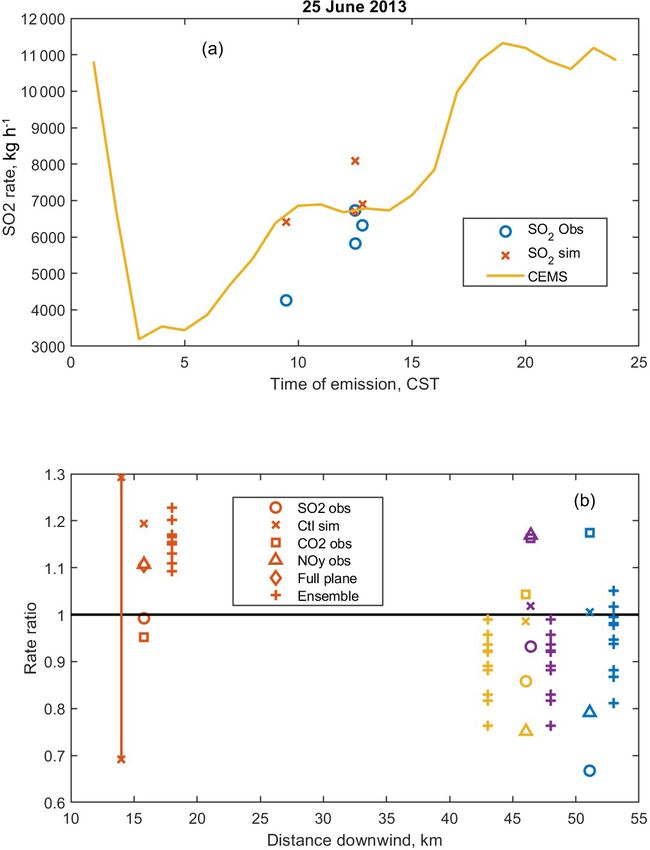
11858                                                     W. M. Angevine et al.: Errors in top-down estimates of emissions

plant plume. We generally use the interpolation method here,     ten found above the boundary layer height specified to the
and our background uncertainty assumptions are further sup-      simulation because the model is designed to allow trans-
ported by multiple years of regional transects upwind and        port above the boundary layer and also because the boundary
downwind of the Martin Lake power plant that reveal few          layer height changes in space and time. It is difficult to tell,
point sources of SO2 , NOx , and CO2 of a magnitude to inter-    however, if this accurately reflects vertical mixing in the real
fere with the Martin Lake plumes in this region. At least one    world.
transect across the plume is made at a height well within the       Fully model-based retrievals of emissions from concentra-
mixed layer. The mixed layer height is usually determined by     tion measurements are usually done with a Bayesian analy-
examining temperature, potential temperature, and trace gas      sis in order to overcome the under-constrained nature of the
concentrations during vertical profiles at the ends of some      problem. A Lagrangian dispersion model is run backwards
transects. More elaborate methods involve multiple down-         in time from the sites of measurements to produce footprints,
wind transects, often accompanied by 2-D interpolation of        which are convolved with a prior inventory. The differences
downwind measurements (Mays et al., 2009). Detailed anal-        between modeled and measured concentrations are then op-
ysis of related methods in the context of column measure-        timized by a mathematical algorithm. Weights (error covari-
ments is given by Varon et al. (2018).                           ances) are applied to the measurements and the prior, ex-
   Sources of error are (1) error in determining the mass flow   pressing relative confidence in their correctness. Bayesian
rate through the plane; (2) the emission rate at the source      analysis requires assumptions about the PDF of errors (usu-
may be different than the mass flow rate through the plane;      ally Gaussian, always with zero mean).
and (3) pollutant may be lost to deposition and/or chemical         Here we use hybrid or intermediate methods to examine
transformation. Determining the mass flow rate through the       the consequences of different classes of error. The meteoro-
plane is done by estimating the concentration at each point      logical model (reanalysis) produces full fields of wind speed
in the plane, multiplying by the area to get a linear mass       and direction and of mixing height. The Lagrangian trans-
density and then multiplying by the wind speed perpendic-        port model then produces a full four-dimensional view of the
ular to the plane to obtain a mass flow rate. Usually one or     plume. From these we can calculate the concentrations at the
more transects is flown through a plume during presumably        aircraft location for direct comparison and for standard mass
well-mixed conditions. Thus the concentrations at a single       balance analysis, as in Karion et al. (2019). We can also cal-
height may be used as an estimate for concentrations from        culate other estimates by considering different heights within
the ground to a well-defined mixing height. Errors may arise     the plume, a range of heights, or the whole plume. We can
because the plume is not well mixed, causing concentrations      use measured or modeled mixing heights and measured or
to vary significantly in the vertical direction; the planetary   modeled winds. We can choose whether to be sensitive to
boundary layer height is not well known; or significant mass     horizontal displacement of the plume.
has been transported above the boundary layer. The other            The ECMWF fifth-generation reanalysis (ERA5) (Coper-
source of error is that the mass flow rate through the plane     nicus Climate Change Service (C3S) (2017): ERA5: Fifth
may be significantly different than the emission rate from the   generation of ECMWF atmospheric reanalyses of the
source. This may occur when winds are variable in speed          global climate. Copernicus Climate Change Service Climate
and/or direction in time and/or space.                           Data Store (CDS), https://cds.climate.copernicus.eu/cdsapp#
                                                                 !/home, last access: March 2019) is used to provide meteo-
3.2   Models                                                     rological fields for this study. It consists of a control (high-
                                                                 resolution) run and 10 ensemble members. The control run is
By using a model, we can virtually eliminate errors arising      available hourly on a 0.25◦ × 0.25◦ latitude–longitude grid,
from (1). In the simulated world, simulated concentrations       with 37 pressure levels. The ensemble members are available
and model wind speeds at every point in the plane are known,     every 3 h on a coarser 0.5◦ × 0.5◦ grid.
so there is no need to estimate a mixing height. In addition,       HYSPLIT version 944 was used in this study. HYSPLIT
the emission from the source is also known in the simulated      is a Lagrangian atmospheric transport and dispersion model
world. Thus mismatch between the emission rate from the          developed by the National Oceanic and Atmospheric Admin-
source and the mass flow rate from the analysis plane is only    istration’s Air Resources Laboratory (NOAA ARL) (Stein et
caused by variable winds and can be explored in detail. Un-      al., 2015). Dispersion of a material is simulated by a num-
certainties due to losses to deposition and/or transformation    ber of computational particles which represent a specified
(3) are also eliminated in the simulations.                      amount of mass of material. The computational particles are
   The mass balance method can also be applied to the sim-       advected by the wind field and dispersed by a turbulent com-
ulated fields by using only simulated concentrations from a      ponent which is calculated by the model from meteorological
single transect and the model mixing height. The tracer pro-     data fields.
file is known exactly in the simulated world, but the mixing        HYSPLIT provides a variety of options to optimize for
height may still not be well defined. Tracer profiles may not    different situations. We used the default methods for de-
have a sharp cutoff in the vertical. Significant mass is of-     termining vertical velocity variances (Kantha–Clayson) and

Atmos. Chem. Phys., 20, 11855–11868, 2020                                        https://doi.org/10.5194/acp-20-11855-2020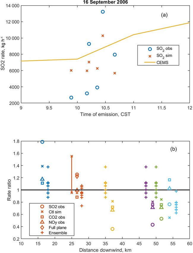
W. M. Angevine et al.: Errors in top-down estimates of emissions                                                               11859

wind and temperature profiles for computing the boundary
layer stability. These are the same settings used by Karion
et al. (2019). The mixed layer depth was taken from the
ERA5 input, which is also the default method. HYSPLIT
was modified to include the Stochastic Time-Inverted La-
grangian Transport (STILT) dispersion algorithm, which was
employed in this study. The STILT dispersion algorithm in-
corporates the Thomson et al. (1997) reflection–transmission
scheme for Gaussian turbulence that preserves well-mixed
distributions for particles moving vertically across interfaces
between grid cells as described in Lin et al. (2003).
   A tracer was emitted from the location of the Martin Lake
stacks (32.26◦ N, −94.57◦ ) at 100 m with the rate given by
the hourly CEMS data for SO2 . Heat content of 8.5 × 10⁷ W
was specified for all simulations and used in the plume rise
calculation.
   Concentrations from HYSPLIT were output on a horizon-
tal grid with increments of 0.011◦ latitude by 0.009◦ longi-
tude, spanning 0.6◦ × 0.8◦ . Vertical levels (25) were spaced
every 100 m up to 2000 m a.g.l. and then every 200 m up to
3000 m a.g.l. HYSPLIT concentrations were output as aver-
ages between each defined level, so for example the first level
in the output is the average between 0 and 100 m a.g.l. The
hourly output represents the average over each hour. No de-
position was used, and the particles were defined as entirely
passive. Ten thousand particles per hour were used to pro-
duce a sufficiently smooth concentration field.

4   Results
                                                                  Figure 1. SO2 mixing ratios (ppbv) observed along four transects
We first examine aircraft observations from the flight on 25      by the aircraft (a) and modeled at the same locations (b) in the con-
June 2013, which took place in good conditions for mass-          trol run on 25 June 2013. The × marks the power plant location.
balance analysis as described above. The plume from the
Martin Lake power plant was intercepted by the aircraft four
times, as shown in Fig. 1. Figure 2 shows the time series         transect to compare with the CEMS measurement. Figure 4
of the observations and the plumes simulated using the con-       shows these results. The CEMS data show that the aircraft
trol meteorology and the 10 ensemble members. The simu-           transects all measured emissions that came out of the stack
lated plume is well aligned with the observations in the first    during a plateau of relatively constant emissions. In the lower
transect but displaced in the other three. Note that the third    panel of Fig. 4, the emission rates are presented as ratios to
and fourth transects were flown in opposite directions. All       the CEMS data for each species. By this means, the three
the simulated plumes are weaker and wider than observed.          measured species constitute separate estimates of the same
There is little visually apparent spread in the ensemble; all     emissions. The single simulated tracer, labeled “SO2 sim”,
the members produce plumes of similar location, magnitude,        serves for all species.
and width. As Fig. 3 shows, however, the integrated amount           Transect 2, at the shortest downwind distance, best meets
of SO2 in the plumes does vary.                                   the mass balance assumptions. The error bar shows the esti-
   The next step is to compute the emission rate represented      mated uncertainty (±30 %, 1 standard deviation) of the ob-
by each transect. This is done by mass balance using ob-          served mass balance estimate. The estimate itself is nearly
served and modeled values separately. The observational           perfect, falling just below the unity ratio line. The simu-
analysis uses the observed mixing ratios, mixing height, and      lated mass balance estimate is about 20 % high, within the
wind speed. Simulated plumes from the control run are ana-        error bar. NOy - and CO2 -observed estimates also fall within
lyzed with the simulated wind speed and mixing height. A          the estimated error (not shown). For the other transects, the
full-plane integration of the simulated plume is also con-        SO2 observed falls consistently below the unity ratio line, al-
ducted and described below. Thus we have a total of three         though only the farthest transect falls outside the error bar.
emission rate estimates from the control simulations for each     The 30 % error estimate is only shown for transect 2, but is

https://doi.org/10.5194/acp-20-11855-2020                                        Atmos. Chem. Phys., 20, 11855–11868, 2020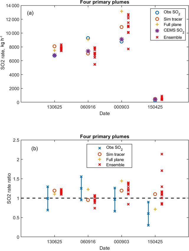
11860 W. M. Angevine et al.: Errors in top-down estimates of emissions
Figure 4. Emission rate estimates from mass balance for four tran-
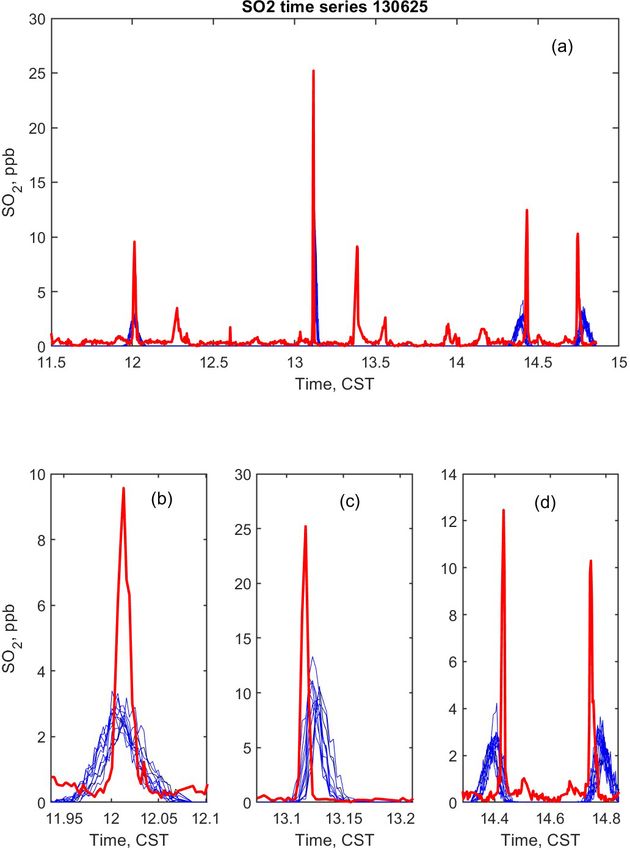
Figure 2. Time series of observed (red) and modeled (control in sects on 25 June 2013. (a) CEMS emission rate through the day with
black, ensemble members in blue) SO2 mixing ratio along the flight observed and simulated emission estimates shown at estimated time
tracks on 25 June 2013. Plots (b, c, d) zoom in on the relevant seg- of emission. (b) Ratio of emission rate derived from different esti-
ments of the upper time series (a) to show details of the plume mag- mates (method and species, symbols as in legend) to CEMS emis-
nitudes and positions. sion at estimated time of emission. Explanation of legend: “obs”
is mass balance using observations; “Ctl sim” is mass balance us-
ing control simulated tracer, wind, and mixing height; “full plane”
is derived by integrating the full x–z plane in the simulation at the
transect latitude; “ensemble” is mass balance using simulated tracer,
wind, and mixing height for each ensemble member. Vertical bar is
uncertainty estimate (1 standard deviation, ±30 %) on observation-
based mass balance for transect 2, and its length applies to all tran-
sects. The four transects are colored blue, red, yellow, and purple
respectively. Ensemble estimates are offset slightly along the x axis
for clarity.
the same for the other transects and species and is described
in more detail in the Discussion section below. NOy and CO2
estimates are scattered but within the 30 % uncertainty esti-
mate. The simulated tracer is nearly perfect for transects 1,
Figure 3. Integrated plume amounts for the four transects on 25 3, and 4, the transects at 45–52 km downwind.
June 2013, comparing observations and simulations. Large circles The set of emission rate estimates resulting from the en-
are from the control simulation, × marks are from the ensemble semble meteorology are shown in Fig. 4 with + marks. For
members. The amounts are found by integrating the mixing ratio in the closest transect (2), the ensemble spread is about 15 %,
time across each of the plumes shown in Fig. 2. less than the estimate of uncertainty for the observations.
The ensemble spread contains the control simulation value
but does not span the unity line. The ensemble estimates for
Atmos. Chem. Phys., 20, 11855–11868, 2020 https://doi.org/10.5194/acp-20-11855-2020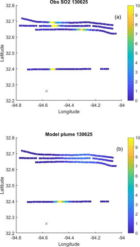
W. M. Angevine et al.: Errors in top-down estimates of emissions                                                            11861

the farther transects have greater spread, although still some-        Another flight with several transects took place on 16
what less than the observation estimate, and all span both the      September 2006 (Fig. 6). Transect 2 has the best match to
control simulation values and unity ratio.                          the mass balance assumptions. The emission rate analysis
   The above mass balance analyses are not sensitive to errors      from observations has a high bias of 25 %, while the es-
in the width or displacement of the plume, since they involve       timate from the control simulation is biased 5 % low. The
integrating across each plume regardless of its exact location      observational estimates for CO2 and NOy are close to their
or width. We can also do an analysis that is insensitive to         respective CEMS values (Table 2). The full-plane estimate
mixing height by integrating the simulated plume in a vertical      agrees closely with the observational estimate for SO2 (Ta-
plane along the flight transect, which we call the full-plane       ble 1). The ensemble estimates have a spread of 36 %, cover
integration. Error in the emission estimate from this method        the CEMS value, and are nearly centered around the control
would arise only from deviations from the assumption of a           simulation value. As for the other transects, the closest tran-
steady mass flow rate through the plane. For transect 2 on 25       sect gives a high-biased observational estimate. The transects
June 2013, the full-plane integration using the control simu-       farther downwind all produce low-biased observational and
lation gives an emission rate of 7500 kg h−1 (Table 1) com-         simulated estimates, except for CO2 and NOy at the farthest
pared to the CEMS value of 6780. This is a bias of 11 %             distance (not shown). The emissions as measured by CEMS
(all percentage values are with respect to the CEMS value).         are increasing during the span of time when the plume was
The full-plane integration using the ensemble meteorology           emitted, adding substantial uncertainty to the comparison.
produces estimates ranging from 6900 to 7500 kg h−1 , with          Examining the vertical cross sections of the plume (Fig. 7),
mean 7130 and median 7140 kg h−1 , a bias of 5 %. The en-           we see that the plume is approximately well mixed at the lat-
semble range of the full-plane estimates does not include the       itude of transect 2 (32.5◦ N) in all but one ensemble member
CEMS value or the observation-based mass balance value,             (em8), but not well mixed at 32.4◦ N, the latitude of tran-
but it does include the control simulation mass balance value.      sect 1.
The ensemble spread is rather small (8 %). The simulated               On 3 September 2000, only one transect is usable (Table 1,
plumes are not perfectly well mixed, with higher concentra-         Fig. 8). The observational analysis produces an emission rate
tions in the lower boundary layer (Fig. 5).                         within 4 % of CEMS. The control simulation overestimates
   The question of mixing height deserves further explo-            by 19 %. The ensemble estimates have substantial spread
ration. Figure 5 shows vertical cross sections in a south–north     (46 %), which covers the values from the observations and
plane, approximately along the wind direction, of the tracer        the control simulation. The full-plane integration has a 44 %
mixing ratios simulated by HYSPLIT with the control mete-           high bias. Some of the difficulty in the simulations is due to
orology and each of the 10 ensemble members. An observed            unrealistically large mixing heights in ERA5. HYSPLIT can-
value of mixing height was subjectively determined from po-         not produce a well-mixed plume in these conditions. Agree-
tential temperature and water vapor profiles flown at the ends      ment between the observational analysis and CEMS reflects a
of the transects, shown as an o mark in each of the subplots. A     reasonable mixing height estimate but may involve some el-
simulated mixing height is estimated from the tracer mixing         ement of good luck. We do not know whether the real plume
ratio profiles. It is the height at which the mixing ratio first    was well mixed. Potential temperature profiles (not shown)
falls below 50 % of its value in the middle height range. It dif-   before the transect show relatively shallow mixing heights
fers for each ensemble member. Another possible source of           consistent with the manual estimate. Observed profiles after
uncertainty in the mixing height is shallow cumulus clouds,         the transect show a deep boundary layer ∼ 2500 m a.g.l., al-
which were present on all four flight days.                         though not as deep as in ERA5 (3000–3600 m). This is an
   Flux estimates for SO2 for all four transects on 25 June         indication that the mixing height was changing during the
2013 are given in numerical form in Table 1. The estimates          time of the observations. Both profiles are at some distance
from observations are within ±14 % for three of the tran-           from the plume location, so their applicability is question-
sects (2, 3, and 4). Simulated values from the control run          able. The emissions measured by CEMS are increasing sub-
are 5 %–19 % high for transects 1, 2, and 4, and 14% low            stantially around the time the plume was emitted, which adds
for transect 3. The observational estimate for transect 1 has       to the uncertainty.
a substantial low bias (34 %), for which we do not have a              The flight on 25 April 2015 took place after the SO2 emis-
convincing explanation.                                             sions of the power plant had been substantially reduced by
   Seeing that the observations and control simulations pro-        scrubbing, so the SO2 plume was much weaker. Analysis of
duce small biases for transects 2, 3, and 4, we now examine         the observations requires estimating the background, and un-
the ensemble simulations. These are shown in Fig. 4, and            certainty in that estimate is more important when the plume
numbers are given in Table 1. The ensemble does not span            is weaker. The observational analysis produces a flux esti-
reality for transect 2, but it does cover the control estimate.     mate biased 40 % low; the control simulation is biased only
The ensemble spread is 12 % for transect 2 and 25 %–36 %            10 % high (Table 1, Fig. 8). The ensemble estimates have
for the other transects.                                            large spreads, more than 100 %. The spread is due mostly to
                                                                    a single high member. We cannot justify removing that mem-

https://doi.org/10.5194/acp-20-11855-2020                                         Atmos. Chem. Phys., 20, 11855–11868, 2020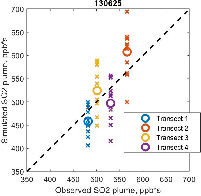
11862 W. M. Angevine et al.: Errors in top-down estimates of emissions
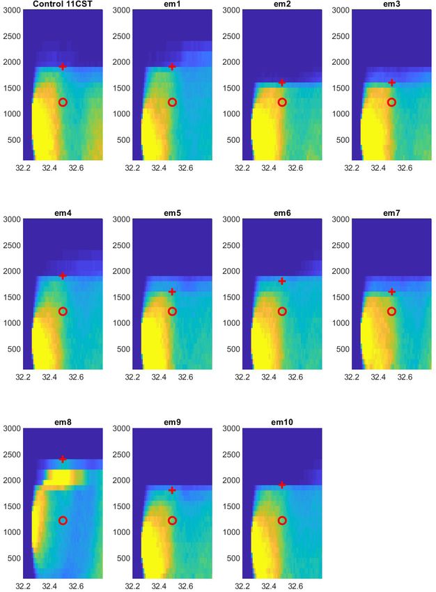
Figure 5. Latitude–height cross sections of SO2 mixing ratio simulated with the control meteorology and each of the ensemble members on
25 June 2013. The cross sections are shown at 13:00 CST. The color scale is linear and is allowed to saturate near the source. Two estimates
of the mixing height are shown at the latitude of transect 2: observed (o, one value for all subplots) and determined from the concentration
profile (+). See text for details.
ber, which is not obviously wrong. Wind speed is biased low 5 Discussion
and mixing height is biased high in the simulations (Table 3).
Several members produce concentration profiles that are not In this section, we use the collection of emissions estimates
well mixed at the observation plane (not shown). Potential described above to explore the uncertainty of such estimates.
temperature profiles before and after the transect (not shown) Several approaches are used:
are consistent with the respective model and observed bound- 1. manual uncertainty estimates for the observational mass
ary layer heights. balance;
2. errors from the observational mass balance for the four
flights, including multiple species;
Atmos. Chem. Phys., 20, 11855–11868, 2020 https://doi.org/10.5194/acp-20-11855-2020W. M. Angevine et al.: Errors in top-down estimates of emissions 11863
Table 2. CEMS and observed emission rates for SO2 , NOy , and CO2 for the four primary transects. SO2 values are repeated from Table 1.
Date CEMS SO2 Mass balance CEMS NOx Mass balance CEMS CO2 Mass balance
(yyyymmdd) rate (kg h−1 ) SO2 rate (bias) rate (kg h−1 ) NOx rate (bias) rate (kg h−1 ) CO2 rate (bias)
20130625 6780 6727 1610 1782 2.51e6 2.39e6
(transect 2) (−7.8 %) (11 %) (−4.7 %)
20060916 7403 9273 1950 1941 2.55e6 2.25e6
(transect 2) (25 %) (−0.5 %) (−12 %)
20000903 9105 8773 3173 3077 2.40e6 2.53e6
(transect 1) (−3.6 %) (−3.0 %) (5.4 %)
20150425 418 251 398 132 4.21e5 3.26e5
(transect 2) (−40 %) (−67 %) (−23 %)
Table 3. Values and ranges of wind speed and mixing height in the simulations and their biases with respect to the observed values.
Date Wind speed mean Wind speed Mixing height Mixing height
(yyyymmdd) (m s−1 ) (bias) ensemble range (m) (bias) ensemble range
20130625 6.4 1.4 1900 500
(transect 2) (−0.77, −11 %) (21 %) (170, 9.8 %) (26 %)
20060916 5.1 0.95 1617 800
(transect 2) (−1.8, −26 %) (19 %) (398, 33 %) (44 %)
20000903 4.7 1.5 1900 1300
(transect 1) (−0.88, −16 %) (32 %) (681, 56 %) (58 %)
20150425 5.5 1.3 1600 600
(transect 2) (−1.7, −23 %) (23 %) (614, 62 %) (43 %)
3. errors from the simulated mass balance for the four the boundary layer depth (±200 m), and the wind speed
flights; (±1 m s−1 ). This results in a total 1σ uncertainty between
±22 % and ±32 % for the emission estimates presented here.
4. errors from the simulated full-plane integrations for the
For clarity of presentation in Figs. 4 and 6, this is represented
four flights;
by a ±30 % error bar.
5. errors from simulated mass balance using the meteoro-
logical ensemble. 5.1 Errors in individual flights
Uncertainty estimates for mass balance calculations from
observations alone are described in detail by Peischl et Of the transects in Table 1, many have large biases, but these
al. (2015, 2018) for the Haynesville Shale area, which in- problematic transects are either far from the source or very
cludes the Martin Lake power plant, using the same flight close. We chose one “primary” transect for each day, flown
data used here for 25 June 2013 and 25 April 2015. They es- at a roughly optimal distance from the source. The primary
timate uncertainties of 300 m (about 20 %) for mixing height transects are highlighted in Table 1, and emissions of all three
and about 28 % for wind speed. These are the dominant un- species are included in Table 2. Because the simulation uses a
certainties in their presentation. Combined, all sources yield passive tracer, values scaled to the CEMS emission rates are
flux uncertainties (for methane from the oil and gas field) of applicable to all three species. Of these four transects, three
about 35 %. We refer to these as the “manual” uncertainty es- have observational estimates within the manually estimated
timates (list item 1 above). We estimate the total uncertainty uncertainty for all three species. The outlying observational
in the mass balance emission rate by summing in quadra- estimate, for 25 April 2015, is subject to uncertainty in the
ture the following sources of uncertainty: the accuracy of background, which may be underestimated, and which does
the gas species measurement (±0.10 ppmv + 3 % in 2000, not affect the simulations. The CO2 observational estimate
±0.15 ppmv otherwise for CO2 ; ±10 % for SO2 , ±12 % for is within the uncertainty on this day. It is not clear how to
NOy ); the background determination of the gas species mea- rigorously combine uncertainties for different flight days and
surement (±20 % for CO2 ; ±5 % for SO2 ; ±10 % for NOy ), species, so we do not present a single number for this collec-
https://doi.org/10.5194/acp-20-11855-2020 Atmos. Chem. Phys., 20, 11855–11868, 202011864 W. M. Angevine et al.: Errors in top-down estimates of emissions
ever, this reduces the error in only two of the four cases. The
error in mixing height must be offsetting an error due to un-
steady winds in the other two cases. The collection suggests
a lower limit of 30 % or so on the uncertainty.
Estimating probabilities or confidence intervals from small
ensembles is challenging (Leutbecher, 2019; Wilks, 2011).
Too few members will generally produce too small a spread.
Ensemble spread is often expressed as a standard deviation,
but if each member is equally likely, the range is a better
measure. Even so, most ensembles have too little spread
and do not encompass the true value. If biases occur, for
example because of model errors common to all members,
the spread probably should not encompass the true value. In
other words, increased random spread is not an adequate sub-
stitute for diagnosis and correction of biases. Bias correction
as part of ensemble calibration should be used. However, suf-
ficient and reliable observations are often unavailable with
which to correct biases, as is the case here.
The example of 25 June 2013 transect 2 is instructive (Ta-
ble 1). Emission rates from the ensemble have a range of
12 % but do not cover the true value. If we call the ensem-
ble range the uncertainty of the rate estimate, it would be too
small (overconfident). If we used the ensemble standard devi-
ation, the uncertainty estimate would be even smaller, about
5 %, which is clearly unreasonable. For the same transect (25
June 2013 transect 2) the rate calculated from observations
is 8 % low relative to reality, and the rate calculated from the
Figure 6. Emission rate estimates from mass balance for six tran- control simulation is 19 % high. Both estimates fall within
sects on 16 September 2006. (a) CEMS SO2 emission rate with ob- the estimated uncertainty of the manual analysis.
served and simulated emission estimates shown at estimated time
Taking the other primary transects in order starting with
of emission. (b) Ratio of emission rate derived from different es-
timates (method and species) to CEMS emission at estimated time
the worst control flux estimate, for 3 September 2000 we
of emission. Explanation of legend: “obs” is mass balance using ob- have a 19 % high bias. The ensemble range is 46 %. These
servations; “Ctl sim” is mass balance using control simulated tracer, differences suggest a somewhat larger uncertainty than the
wind, and mixing height; “full plane” is derived by integrating the manual estimate. Other clues to problems with this plume
full x–z plane in the simulation at the transect latitude; “ensemble” include very high boundary layer height from ERA5 and a
is mass balance using simulated tracer, wind, and mixing height large difference between mixing heights estimated from the
for each ensemble member. Vertical bar is uncertainty estimate (1 aircraft profiles before and after the transect. However, if
standard deviation, ±30 %) on observation-based mass balance for mixing height were the only problem, the full-plane integra-
transect 2. The six transects are colored blue, red, yellow, purple, tion would produce a correct estimate, since it is not sensi-
green, and cyan respectively. Ensemble estimates are offset slightly tive to mixing height or to the well-mixed assumption. The
along the x axis for clarity.
remaining source of error is the variability of the winds lead-
ing to storage of pollutant within the volume between the
source and the measurement plane, which accounts for the
tion (list item 2 above). An uncertainty estimate of less than rest of the bias (control) and spread (ensemble). The winds
23 % would leave four outliers rather than two. We therefore were light and variable during the night and early morning.
choose an estimate of approximately 25 % to avoid being too Transect 2 on 16 September 2006 has emission rate esti-
optimistic. mates from the observations that are 25 % high and from the
All four estimates for SO2 from the primary transects us- control simulation 5 % low. The full-plane integration returns
ing the control simulation are within the manually estimated a 22 % high bias. The ensemble range is 36 % and covers re-
uncertainty (Table 1 and Fig. 8). Again, no rigorous com- ality. The other transects on this day are either too close for
bined uncertainty can be computed (list item 3 above) but the plume to be well mixed (transect 1) or too far away for
anything less than 20 % would be too optimistic, leaving out the assumption that SO2 is roughly conserved to be valid.
two of the four estimates. The full-plane integration (list item Transect 2 on 25 April 2015 has already been mentioned
4) eliminates one source of uncertainty, the estimation of as suffering from background uncertainty. The control-based
mixing height. Somewhat counter to our expectation, how- estimate is close to reality. The full-plane integration is bi-
Atmos. Chem. Phys., 20, 11855–11868, 2020 https://doi.org/10.5194/acp-20-11855-2020W. M. Angevine et al.: Errors in top-down estimates of emissions 11865
Figure 7. Latitude–height cross sections of tracer mixing ratio simulated with the control meteorology and each of the ensemble members
on 16 September 2006. The cross sections are shown at 11:00 CST. The color scale is linear and is allowed to saturate near the source.
Two estimates of the mixing height are shown at the latitude of transect 2: observed (o, one value for all subplots) and determined from the
concentration profile (+). See text for details.
ased 28 % low, still within the manually estimated uncer- tion, however, that the small range on 25 June 2013 is prob-
tainty. One outlying member produces the very large en- ably underestimated.
semble spreads. There is nothing to justify removing this
member, which again emphasizes the difficulty of estimating 5.2 Main sources of error
spread from a small number of members.
Overall, the ensemble ranges give uncertainty estimates of Mixing height and the well-mixed assumption are important
12 %–105 % on different days (list item 5). This is informa- uncertainties in the mass balance framework (White et al.,
tion that cannot be obtained in any other way. We must cau- 1983; Karion et al., 2019). This is not very surprising con-
sidering that the definition of a single mixing height involves
several unsafe assumptions. For the boundary layer to be well
https://doi.org/10.5194/acp-20-11855-2020 Atmos. Chem. Phys., 20, 11855–11868, 202011866 W. M. Angevine et al.: Errors in top-down estimates of emissions
an aircraft will typically perform multiple vertical profiles,
probing the mixing height and how it evolves throughout the
study period, and will transect the plume at different altitudes
(Peischl et al., 2015).
Wind speed is another important uncertainty. The usual as-
sumption is that the wind speed at the measurement transect
is representative for the entire plume transit. If the wind is
light and therefore variable, or if the wind speed has changed
substantially over the transit time, it is unclear what wind
speed to use in the calculation. Sometimes modeled wind
speeds are used (Karion et al., 2015). Looking at Table 3, we
see substantial biases in wind speed (low) and mixing height
(high), the smallest biases occurring on 25 June 2013. These
biases are with respect to the winds and mixing height ob-
served on the aircraft, and therefore also include substantial
uncertainties. The ensemble ranges can be compared with the
manual estimates of uncertainty. For wind speed, the ensem-
ble ranges are comparable to the manual estimates or smaller.
For mixing height, the ensemble ranges are larger. Combin-
ing simulated and observed values, for example using simu-
lated wind speeds with observed mixing heights, would incur
large errors.
The methods used here are not sensitive to some com-
mon sources of error. None of these methods are sensitive
to plume displacement caused by errors in wind direction, as
long as the plume is fully covered by the transect. The full-
plane integration is not sensitive to the mixing height estima-
Figure 8. Emission rate estimates from mass balance for the four tion or to violations of the well-mixed assumption. The fact
primary transects highlighted in Table 1. (a) Absolute SO2 emis- that the full-plane estimate is farther from reality than the tra-
sion rates. (b) Ratio of SO2 emission rates derived from different ditional mass balance estimate for three of the four primary
estimates (method and species) to CEMS emission at estimated time transects suggests that compensating errors are present. Sig-
of emission. Explanation of legend: “obs” is mass balance using ob- nificant uncertainties remain in all methods.
servations; “sim” is mass balance using simulated tracer, wind, and This work was partly inspired by the study of Karion et
mixing height; “full plane” is derived by integrating the full x–z
al. (2019). The main emphasis of that work was on large (fac-
plane in the simulation at the transect latitude; “ensemble” is mass
tor of 2 or greater) biases due primarily to errors in vertical
balance using simulated tracer, wind, and mixing height for each en-
semble member. Vertical bar is uncertainty estimate on observation- mixing in the Lagrangian transport models. We should keep
based mass balance. in mind, however, that the true emissions in that study are not
known. The true vertical mixing is not known in either that
study or this one. Karion et al. (2019) also reported large un-
mixed, there must be a substantial surface buoyancy flux, a certainties (error bars) based on multiple flights and multiple
well-defined capping layer (not necessarily an inversion per models. Variability from a small ensemble of meteorology in
se), and minimal change of advection with height. Bound- one configuration (WRF2-FP) was 20 %–30 %.
ary layers are commonly well mixed in potential tempera- An earlier study by Angevine et al. (2014) used a six-
ture but not in water vapor mixing ratio (Gao et al., 2018), member WRF ensemble driving forward runs of the Flexible
because the entrainment fluxes at the top of the boundary Particle (FLEXPART) Lagrangian dispersion model to esti-
layer are of opposite sign (warming for temperature, dry- mate uncertainty due to meteorology. A passive tracer rep-
ing for water vapor). Additional conditions are required for resenting national inventory emissions of carbon monoxide
a plume to be well mixed; specifically, there must be enough (CO) was transported by the models. That study found 30 %–
time (several boundary layer turnover times) between emis- 40 % spread in CO concentrations. The ensemble spread was
sion and measurement. It is worth noting that plumes that are insufficient to cover the errors in wind and temperature, as
not well mixed can sometimes give reasonable mass balance would be expected for a small ensemble using a single model
estimates if the measurement transect is flown close to the framework.
middle of the boundary layer, where the measured value ap-
proximates the mean of the (roughly linear) vertical profile.
To reduce these uncertainties in the mass balance calculation,
Atmos. Chem. Phys., 20, 11855–11868, 2020 https://doi.org/10.5194/acp-20-11855-2020W. M. Angevine et al.: Errors in top-down estimates of emissions 11867
6 Conclusions sible for any use that may be made of the Copernicus information
or data it contains.
Errors in top-down emissions estimates are substantial even
under good conditions. Using a known source in forward Author contributions. WMA and JP designed the study. JP did the
runs driven by ensemble meteorology, we have shown er- observational mass flux analysis including its uncertainties. WMA
rors ranging from a few percent to over 100 %. No single ran the HYSPLIT model with help from AC and CPL. WMA an-
robust estimate of either bias or random error can be derived alyzed the model results and wrote the paper with input from the
from these results. Identification and removal of cases that coauthors. IBP and CRT were involved in taking the measurements.
are clearly bad reduces the error, but if the source is un-
known, some bad cases cannot be clearly identified. Inves-
Competing interests. The authors declare that they have no conflict
tigator judgment is vital. Using forward modeling and exam-
of interest.
ining the structure of the plumes it produces can be helpful
in identifying better or worse cases. Using an ensemble pro-
vides another dimension for diagnosis, since the spread of Acknowledgements. We are grateful for many enlightening discus-
the ensemble results can indicate the possibility of outlying sions with Michael Trainer and Anna Karion. John Holloway, David
solutions that are not apparent in a single deterministic run. Parrish, Steven Sjostedt, and Thomas Ryerson were involved in tak-
The largest source of error is the vertical mixing, as was ing the measurements in one or more of the flights used here.
also shown by Karion et al. (2019). This is not simply a ques-
tion of finding a correct mixing height, although that is a ma-
jor problem. In several of the cases shown here, the plumes Financial support. This research has been supported by the NOAA
are not well mixed, and the mixing height is therefore not Chemical Sciences Laboratory.
well defined.
Wind speed is another important source of error (Table
3). The wind speed on the aircraft transect may be the only Review statement. This paper was edited by Andreas Hofzumahaus
source of data for comparison to the models. However, even and reviewed by three anonymous referees.
if it compares perfectly, unsteadiness of the wind previous to
the measurement can cause poorly characterized errors.
Losses of pollutant to deposition or chemical transforma-
References
tion can be important for observations taken at longer down-
wind distances (greater than ∼ 20 km), as seen in Figs. 4 and Angevine, W. M.: Supporting data, https://esrl.noaa.gov/csl/groups/
6. These losses can be estimated if sufficient information is csl4/modeldata/, last access: 9 October 2020.
available, for example measurements of product species, but Angevine, W. M., Brioude, J., McKeen, S., and Holloway, J. S.:
those estimates will necessarily introduce additional uncer- Uncertainty in Lagrangian pollutant transport simulations due
tainty. to meteorological uncertainty from a mesoscale WRF ensemble,
These results are not sensitive to errors in plume location Geosci. Model Dev., 7, 2817–2829, https://doi.org/10.5194/gmd-
or width. In future work, we will explore the sensitivity of 7-2817-2014, 2014.
Bayesian inversion methods to those errors as well as to the Gao, Z., Liu, H., Li, D., Katul, G. G., and Blanken, P. D.: En-
kinds of errors shown here. hanced temperature-humidity similarity caused by entrainment
processes with increased wind shear, J. Geophys. Res., 123,
Our results are consistent with uncertainty estimates from
4110–4121, https://doi.org/10.1029/2017JD028195, 2018.
rigorous analysis of observations, as performed by Peischl et Hsu, Y.-K., VanCuren, T., Park, S., Jakober, C., Herner, J., FitzGib-
al. (2015). The minimum emissions flux uncertainty that can bon, M., Blake, D. R., and Parrish, D. D.: Methane emissions
be supported by these results is 30 %. Under less than ideal inventory verification in southern California, Atmos. Environ.,
conditions, errors can be much larger. 44, 1–7, https://doi.org/10.1016/j.atmosenv.2009.10.002, 2010.
Joint Committee for Guides in Metrology: JCGM 100 – Evaluation
of measurement data – Guide to the expression of uncertainty in
Code and data availability. Observational data used here are avail- measurement, JCGM, 120 pp., 2008.
able from https://esrl.noaa.gov/csl/field.html (last access: 9 Octo- Karion, A., Sweeney, C., Pétron, G., Frost, G., Michael Hardesty,
ber 2020, NOAA Chemical Sciences Laboratory, 2020). The HYS- R., Kofler, J., Miller, B. R., Newberger, T., Wolter, S., Banta, R.,
PLIT model and documentation are available from https://www.arl. Brewer, A., Dlugokencky, E., Lang, P., Montzka, S. A., Schnell,
noaa.gov/hysplit/hysplit/ (last access: 9 October 2020, NOAA Air R., Tans, P., Trainer, M., Zamora, R., and Conley, S.: Methane
Resources Laboratory, 2020). HYSPLIT output used in this work emissions estimate from airborne measurements over a western
is available at https://esrl.noaa.gov/csl/groups/csl4/modeldata/ (last United States natural gas field, Geophys. Res. Lett., 40, 4393–
access: 9 October 2020, Angevine, 2020). The ERA5 analyses were 4397, https://doi.org/10.1002/grl.50811, 2013.
generated using Copernicus Climate Change Service Information Karion, A., Sweeney, C., Kort, E. A., Shepson, P. B., Brewer, A.,
(2019). Neither the European Commission nor ECMWF is respon- Cambaliza, M., Conley, S. A., Davis, K., Deng, A., Hardesty, M.,
https://doi.org/10.5194/acp-20-11855-2020 Atmos. Chem. Phys., 20, 11855–11868, 202011868 W. M. Angevine et al.: Errors in top-down estimates of emissions Herndon, S. C., Lauvaux, T., Lavoie, T., Lyon, D., Newberger, T., Peischl, J., Eilerman, S. J., Neuman, J. A., Aikin, K. C., de Gouw, Pétron, G., Rella, C., Smith, M., Wolter, S., Yacovitch, T. I., and J., Gilman, J. B., Herndon, S. C., Nadkarni, R., Trainer, M., Tans, P.: Aircraft-Based Estimate of Total Methane Emissions Warneke, C., and Ryerson, T. B.: Quantifying Methane and from the Barnett Shale Region, Environ. Sci. Technol., 49, 8124– Ethane Emissions to the Atmosphere From Central and Western 8131, https://doi.org/10.1021/acs.est.5b00217, 2015. U.S. Oil and Natural Gas Production Regions, J. Geophys. Res.- Karion, A., Lauvaux, T., Lopez Coto, I., Sweeney, C., Mueller, K., Atmos., 123, 7725–7740, https://doi.org/10.1029/2018jd028622, Gourdji, S., Angevine, W., Barkley, Z., Deng, A., Andrews, A., 2018. Stein, A., and Whetstone, J.: Intercomparison of atmospheric Ryerson, T., Buhr, M. P., Frost, G. J., Goldan, P. D., Holloway, J., trace gas dispersion models: Barnett Shale case study, Atmos. Huebler, G., Jobson, B. T., Kuster, W. C., McKeen, S., Parrish, D. Chem. Phys., 19, 2561–2576, https://doi.org/10.5194/acp-19- D., Roberts, J. M., Sueper, D. T., Trainer, M., Williams, J., and 2561-2019, 2019. Fehsenfeld, F. C.: Emissions lifetimes and ozone formation in Leutbecher, M.: Ensemble size: How suboptimal is less power plant plumes, J. Geophys. Res., 103, 22569–22583, 1998. than infinity, Q. J. Roy. Meteor. Soc., 145, 107–128, Ryerson, T., Huey, L. G., Knapp, K., Neuman, J. A., Parrish, D. D., https://doi.org/10.1002/qj.3387, 2019. Sueper, D. T., and Fehsenfeld, F. C.: Design and initial character- Lin, J. C., Gerbig, C., Wofsy, S. C., Andrews, A. E., ization of an inlet for gas-phase NOy measurement from aircraft, Daube, B. C., Davis, K. J., and Grainger, C. A.: A near- J. Geophys. Res., 104, 5483–5492, 1999. field tool for simulating the upstream influence of atmo- Stein, A. F., Draxler, R. R., Rolph, G. D., Stunder, B. J. B., Cohen, spheric observations: The Stochastic Time-Inverted Lagrangian M. D., and Ngan, F.: NOAA’s HYSPLIT Atmospheric Transport Transport (STILT) model, J. Geophys. Res., 108, 4493, and Dispersion Modeling System, B. Am. Meteorol. Soc., 96, https://doi.org/10.1029/2002JD003161, 2003. 2059–2077, https://doi.org/10.1175/bams-d-14-00110.1, 2015. Mays, K. L., Shepson, P. B., Stirm, B. H., Karion, A., Sweeney, C., Thomson, D. J., Physick, W. L., and Maryon, R. H.: Treatment of and Gurney, K. R.: Aircraft-Based Measurements of the Carbon interfaces in random walk dispersion models, J. Appl. Meteorol., Footprint of Indianapolis, Environ. Sci. Technol., 43, 7816–7823, 36, 1284–1295, 1997. https://doi.org/10.1021/es901326b, 2009. Trainer, M., Ridley, B. A., Buhr, M. P., Kok, G., Walega, J., NOAA Chemical Sciences Laboratory: Field campaigns, avail- Hübler, G., Parrish, D. D., and Fehsenfeld, F. C.: Regional ozone able at: https://esrl.noaa.gov/csl/field.html, last access: 9 October and urban plumes in the southeastern United States: Birming- 2020. ham, A case study, J. Geophys. Res.-Atmos., 100, 18823–18834, NOAA Air Resources Laboratory: HYSPLIT, available at: https: https://doi.org/10.1029/95JD01641, 1995. //www.arl.noaa.gov/hysplit/hysplit/, last access: 9 October 2020. Turnbull, J. C., Karion, A., Fischer, M. L., Faloona, I., Guilder- Palmer, T.: The ECMWF ensemble prediction system: Looking son, T., Lehman, S. J., Miller, B. R., Miller, J. B., Montzka, S., back (more than) 25 years and projecting forward 25 years, Q. J. Sherwood, T., Saripalli, S., Sweeney, C., and Tans, P. P.: Assess- Roy. Meteor. Soc., 145, 12–24, https://doi.org/10.1002/qj.3383, ment of fossil fuel carbon dioxide and other anthropogenic trace 2018. gas emissions from airborne measurements over Sacramento, Peischl, J., Ryerson, T. B., Holloway, J. S., Parrish, D. D., California in spring 2009, Atmos. Chem. Phys., 11, 705–721, Trainer, M., Frost, G. J., Aikin, K. C., Brown, S. S., Dubé, https://doi.org/10.5194/acp-11-705-2011, 2011. W. P., Stark, H., and Fehsenfeld, F. C.: A top-down anal- Varon, D. J., Jacob, D. J., McKeever, J., Jervis, D., Durak, ysis of emissions from selected Texas power plants during B. O. A., Xia, Y., and Huang, Y.: Quantifying methane Texas 2000 and 2006, J. Geophys. Res.-Atmos., 115, D16303, point sources from fine-scale satellite observations of atmo- https://doi.org/10.1029/2009JD013527, 2010. spheric methane plumes, Atmos. Meas. Tech., 11, 5673–5686, Peischl, J., Ryerson, T. B., Holloway, J. S., Trainer, M., An- https://doi.org/10.5194/amt-11-5673-2018, 2018. drews, A. E., Atlas, E. L., Blake, D. R., Daube, B. C., Dlu- White, W. H., Anderson, J. A., Blumenthal, D. L., Husar, R. gokencky, E. J., Fischer, M. L., Goldstein, A. H., Guha, A., B., Gillani, N. V., Husar, J. D., and Wilson, W. E.: For- Karl, T., Kofler, J., Kosciuch, E., Misztal, P. K., Perring, A. mation and transport of secondary air pollutants: ozone and E., Pollack, I. B., Santoni, G. W., Schwarz, J. P., Spackman, aerosols in the St. Louis urban plume, Science, 194, 187, J. R., Wofsy, S. C., and Parrish, D. D.: Airborne observations https://doi.org/10.1126/science.959846, 1976. of methane emissions from rice cultivation in the Sacramento White, W. H., Patterson, D. E., and Wilson Jr., W. E.: Ur- Valley of California, J. Geophys. Res.-Atmos., 117, D00V25, ban exports to the nonurban troposphere: Results from https://doi.org/10.1029/2012JD017994, 2012. Project MISTT, J. Geophys. Res.-Oceans, 88, 10745–10752, Peischl, J., Ryerson, T. B., Aikin, K. C., de Gouw, J. A., Gilman, https://doi.org/10.1029/JC088iC15p10745, 1983. J. B., Holloway, J. S., Lerner, B. M., Nadkarni, R., Neuman, Wilks, D. S.: Statistical methods in the atmospheric sciences, Third J. A., Nowak, J. B., Trainer, M., Warneke, C., and Parrish, ed., Academic Press, Oxford, 676 pp., 2011. D. D.: Quantifying atmospheric methane emissions from the Haynesville, Fayetteville, and northeastern Marcellus shale gas production regions, J. Geophys. Res.-Atmos., 120, 2119–2139, https://doi.org/10.1002/2014JD022697, 2015. Atmos. Chem. Phys., 20, 11855–11868, 2020 https://doi.org/10.5194/acp-20-11855-2020
You can also read