WP/20/67 Effects of Macroprudential Policy: Evidence from Over 6,000 Estimates - International Monetary Fund
←
→
Page content transcription
If your browser does not render page correctly, please read the page content below
WP/20/67

Effects of Macroprudential Policy: Evidence from Over 6,000
                                                  Estimates

    by Juliana Araujo, Manasa Patnam, Adina Popescu, Fabian Valencia and Weijia Yao

 IMF Working Papers describe research in progress by the author(s) and are published
 to elicit comments and to encourage debate. The views expressed in IMF Working Papers
 are those of the author(s) and do not necessarily represent the views of the IMF, its
 Executive Board, or IMF management.
© 2020 International Monetary Fund                                                             WP/20/67

                                       IMF Working Paper

                             Strategy, Policy and Review Department

           Effects of Macroprudential Policy: Evidence from Over 6,000 Estimates 1

     Prepared by Juliana Araujo, Manasa Patnam, Adina Popescu, Fabian Valencia and
                                      Weijia Yao

                          Authorized for distribution by Vikram Haksar

                                              May 2020

    IMF Working Papers describe research in progress by the author(s) and are published to
    elicit comments and to encourage debate. The views expressed in IMF Working Papers are
    those of the author(s) and do not necessarily represent the views of the IMF, its Executive Board,
    or IMF management.

                                               Abstract

This paper builds a novel database on the effects of macroprudential policy drawing from 58
empirical studies, comprising over 6,000 results on a wide range of instruments and outcome
variables. It encompasses information on statistical significance, standardized magnitudes, and other
characteristics of the estimates. Using meta-analysis techniques, the paper estimates average effects
to find i) statistically significant effects on credit, but with considerable heterogeneity across
instruments; ii) weaker and more imprecise effects on house prices; iii) quantitatively stronger
effects in emerging markets and among studies using micro-level data; and iv) statistically
significant evidence of leakages and spillovers. Other findings include relatively stronger impacts
for tightening than loosening actions and negative effects on economic activity in the near term.

JEL Classification Numbers: E28, G28.
Keywords: Macroprudential Policy, financial stability, Meta-analysis.
Authors’ E-Mail Addresses: jaraujo@imf.org; mpatnam@imf.org; apopescu@imf.org;
fvalencia@imf.org; wyao@imf.org.

1
  The authors would like to thank Tamim Bayoumi, Gaston Gelos, Gita Gopinath, Lucyna Gornicka, Vikram
Haksar, Mahmut Kutlukaya, Maria Soledad Martinez Peira, seminar participants at the IMF, and numerous
authors who graciously shared additional results and data from their papers which made it feasible to
standardize results and enhance comparability of estimates.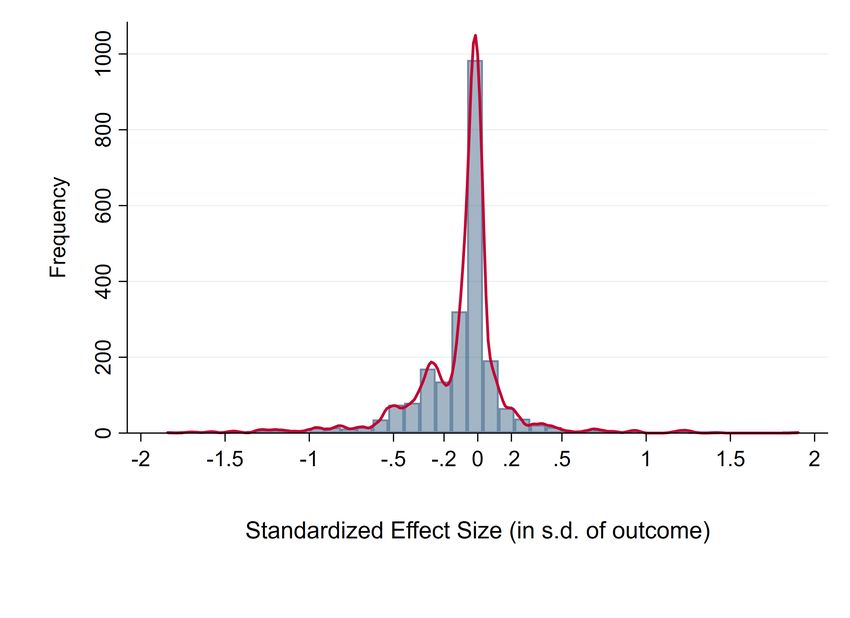
2

                                                        Contents                                                                                         Page

I.    Introduction . . . . . . . . . . . . . . . . . . . . . . . . . . . . . . . . . . . . . .                                                                3
II.   Construction of the Database . . . . . . . . . . .                             .   .   .   .   .   .   .   .   .   .   .   .   .   .   .   .   .   .   5
      A. Paper Selection . . . . . . . . . . . . . . . .                             .   .   .   .   .   .   .   .   .   .   .   .   .   .   .   .   .   .   5
      B. Estimates and Statistics Selection . . . . . .                              .   .   .   .   .   .   .   .   .   .   .   .   .   .   .   .   .   .   6
      C. MPM’s and Outcome Variables Classification                                  .   .   .   .   .   .   .   .   .   .   .   .   .   .   .   .   .   .   7
      D. MPM’s Measurement . . . . . . . . . . . .                                   .   .   .   .   .   .   .   .   .   .   .   .   .   .   .   .   .   .   8
      E. Standardization . . . . . . . . . . . . . . . .                             .   .   .   .   .   .   .   .   .   .   .   .   .   .   .   .   .   .   8
III. Descriptive Statistics . . .   .   .   .   .   .    .   .   .   .   .   .   .   .   .   .   .   .   .   .   .   .   .   .   .   .   .   .   .   .   .   10
     A. Database Overview . .       .   .   .   .   .    .   .   .   .   .   .   .   .   .   .   .   .   .   .   .   .   .   .   .   .   .   .   .   .   .   10
     B. Statistical Significance    .   .   .   .   .    .   .   .   .   .   .   .   .   .   .   .   .   .   .   .   .   .   .   .   .   .   .   .   .   .   12
     C. Magnitudes . . . . . .      .   .   .   .   .    .   .   .   .   .   .   .   .   .   .   .   .   .   .   .   .   .   .   .   .   .   .   .   .   .   12
     D. Symmetry . . . . . .        .   .   .   .   .    .   .   .   .   .   .   .   .   .   .   .   .   .   .   .   .   .   .   .   .   .   .   .   .   .   15
IV.   Meta-Regressions . . . . . . . . . . . . . . . . . . . . . . . . . . . . . . . . . .                                                               .   18
      A. Methodology . . . . . . . . . . . . . . . . . . . . . . . . . . . . . . . . . .                                                                 .   18
      B. Baseline Results . . . . . . . . . . . . . . . . . . . . . . . . . . . . . . . .                                                                .   20
      C. Heterogeneity of Average Effects . . . . . . . . . . . . . . . . . . . . . . .                                                                  .   23
      D. Reconciling Macro and Micro Estimates: Statistical Power and Leakages and
          Spillovers . . . . . . . . . . . . . . . . . . . . . . . . . . . . . . . . . . . .                                                             . 26
      E. Impact on Economic Activity . . . . . . . . . . . . . . . . . . . . . . . . .                                                                   . 28
      F. Dynamics . . . . . . . . . . . . . . . . . . . . . . . . . . . . . . . . . . . .                                                                . 30
V.    Conclusion . . . . . . . . . . . . . . . . . . . . . . . . . . . . . . . . . . . . . . 31
References . . . . . . . . . . . . . . . . . . . . . . . . . . . . . . . . . . . . . . . . . . 33
Appendices . . . . . . . . . . . . . . . . . . . . . . . . . . . . . . . . . . . . . . . . . 39
VI. Testing for Selection bias . . . . . . . . . . . . . . . . . . . . . . . . . . . . . . . 40
VII. Additional Results . . . . . . . . . . . . . . . . . . . . . . . . . . . . . . . . . . . 41
VIII. Robustness . . . . . . . . . . . . . . . . . . . . . . . . . . . . . . . . . . . . . . . 43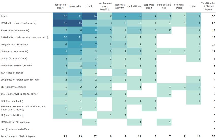
3

                                           I. I NTRODUCTION

Macroprudential policy has by now been deployed in over one hundred countries using a
wide range of instruments (Alam and others, 2019; Cerutti, Claessens, and Laeven, 2017).
The prominence of its use has grown over the years, with more recent actions concentrated in
relaxation measures as part of the policy response to the COVID-19 pandemic to support the
flow of credit to the real economy (Benediktsdóttir, Feldberg, and Liang, 2020; IMF, 2020).

However, there is still limited consensus on how well the toolkit works in practice, and even
less on which instruments work best, despite the rapidly increasing empirical literature on its
effectiveness.1 While considerable empirical work has so far been conducted, the pieces of
evidence remain fragmented.

This paper aims to fill this gap by constructing a novel database of empirical findings on the
effects of macroprudential policy and undertaking a forensic examination of the existing
evidence. The database comprises 6,627 results from fifty-eight papers, selected through a
systematic approach, split evenly between cross-country and country-specific studies. The
database captures information on the effects of macroprudential policies by (i) outcome vari-
able, (ii) instrument, (iii) measurement of macroprudential policy, (iv) categories of controls
(v) time horizon of effect, (vi) sample (i.e. country and period) and (vii) methodology and
unit of analysis. In addition to the actual estimated coefficients, it also includes standardized
coefficients (i.e. effects expressed in standard deviations of the outcome variable), to ensure
comparability across studies. The database is available through the accompanying data file.

The paper then summarizes the effects of macroprudential policy on the most widely studied
outcomes. Extracting a summary view and deriving an “average” effect requires an approach
that combines information about precision of estimates and their magnitudes. To this end,
the paper uses a meta-analysis framework, to quantitatively synthesize research on policy
effects and examine how this average vary with some study or results characteristics. The
paper focuses on the following specific questions: what are the average effects of macropru-
dential policies on credit, household credit, and house prices? How do these average effects
vary by, either the type of instrument deployed, the country setting, or the unit of analysis
(macro-level vs. micro-level data)? In answering these questions, the paper also looks at the
unintended effects that may arise due to leakages or spillovers (e.g., through cross-border or
non-bank lending) or costs from reducing economic activity.

The paper finds that a tightening of macroprudential policy has statistically significant effects
on credit, with stronger effects found for liquidity measures, with considerable variation in
the distribution of these effects across tools and outcomes; for instance, tightening limits on
loan-to-value (LTV) or debt-service-to-income (DSTI) ratios produce similar average effects
1 While  in theory there are strong arguments why macroprudential policy should work, in practice there can also
be factors such as circumvention that could undermine its effectiveness (Bengui and Bianchi, 2018) or general
equilibrium effects that may present trade-offs potentially rendering the net effects of macroprudential policy
ambiguous (Agénor, 2019). This ambiguity means that the overall effectiveness of macroprudential policy is
ultimately an empirical question, and thus a growing body of literature attempts to shed light on it.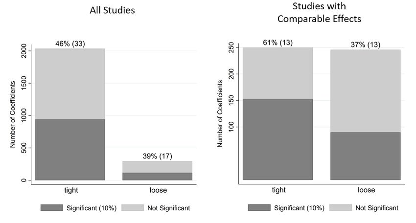
4

on reducing household credit but have weaker and imprecise effects on house prices.2 The
paper also finds that housing and liquidity-based measures appear to have larger average
effects, but with wider confidence bands, in emerging markets. Overall, these findings are
robust to controlling for selection bias, and whether studies are published in a peer-reviewed
journal.3

Furthermore, the average effects are up-to three times larger among studies using micro-level
data than those found in studies using aggregate data. This could be partly explained by the
stronger identification power provided by micro-level data or the existence of spillovers and
leakages which reduce the transmission of the micro-level effects of macroprudential policy
on bank lending to aggregate credit. The paper also finds statistically significant average
leakages and spillover effects, which is consistent with the hypothesis that international banks
or other unconstrained institutions may respond to domestic credit demand when local banks
become constrained (Reinhardt and Sowerbutts, 2015).

Beyond leakages and spillovers, the paper also documents statistically significant and neg-
ative effects on economic activity, at least in the near term. When considering symmetry of
effects (i.e. tightening versus easing macroprudential measures), there is a somewhat larger
body of evidence supportive of more significant and quantitatively stronger effects for tight-
ening than loosening actions. Finally, the literature also documents a persistent impact of
macroprudential policies, but with a large fraction of effects observed within the first year.
Several papers in the database also document how the effects of macroprudential policy vary
depending on financial and macroeconomic conditions. However, summarizing these and
other non-linearities comprehensively requires additional information that was not included in
any of the papers in the database, as explained later in Section II.

This paper contributes to the broader empirical literature on the effects of macroprudential
policy which has predominantly focused on testing whether the adjustment and/or adop-
tion of macroprudential policy tools affects outcomes that could signal the buildup of sys-
temic risk such as credit growth, household leverage and house prices (e.g. Alam and others,
2019; Cerutti, Claessens, and Laeven, 2017; Claessens, Ghosh, and Mihet, 2013). A few
studies explore the effects of macroprudential policy on the probability of a banking crisis
(e.g. Crowe and others, 2012); other studies also provide supporting evidence of unintended
consequences, such as a negative impact on economic activity (e.g. Richter, Schularick, and
Shim, 2019) or leakages and spillovers (e.g. Ahnert and others, 2018; Aiyar, Calomiris, and
Wieladek, 2014). However, getting a comprehensive picture of what the literature finds re-
quires going well beyond a selective and qualitative review.

This paper provides a novel comprehensive synthesis of the evidence on macroprudential
policies. Previous related studies include (Galati and Moessner, 2013, 2018), who conduct a
narrative review of the literature, and Gambacorta and Murcia (2019), who conduct a focused
2 The   meta-analysis focuses on results where the macroprudential policy variable is measured through dummies
reflecting loosening, hold, or tightening actions, which represent the majority of the results in the database.
 3 Quality of papers and results is addressed in several ways, including by controlling for selection bias, journal

of publication, and completeness of the econometric specification within each paper, among others explained
later in the paper.
5

meta-analysis of 7 studies.4 While building on these existing reviews, this paper considerably
expands the scale (from 15 to 58 papers) and scope of the review, covering also leakages and
spillovers and economic costs. Further, in contrast to narrative literature reviews, this paper
uses meta-analysis techniques based employing objective procedures for the selection of
studies to avoid any biases that could ultimately influence the conclusions. These techniques
also allow examining the factors driving the heterogeneity across results (Stanley, 2001).

The next section describes the construction of the database (Section II), followed by descrip-
tive statistics in Section III. Section IV.A lays out the methodology for the meta-analysis and
its main results and Section V concludes.

                             II. C ONSTRUCTION OF THE DATABASE

In describing how the database was built, it is useful to start by noting that all empirical stud-
ies in the review estimate the effect of macroprudential policy tool(s), MPM, on an outcome
variable y, after controlling for factors collected in the vector X. The unit of analysis, i, can be
measured using aggregate data (e.g. country level) or micro data (e.g. banks, firms, or loans).
The period of analysis, t, can be one month, quarter, or year.

                                      yit = β̂ · MPMit + ζ · Xit + uit

Because there is no "standard" specification, the literature includes many variations of the
above equation, often involving multiple tools, outcome variables, set of controls, and differ-
ent ways to measure them.

The main goal is to construct summaries of the β , using meta-analysis techniques, for each
outcome variable/MPM tool pair from a systematically selected set of papers. Because of
the significant variation in tools and outcome variables studied in the literature, the scope
of the meta-analysis is comparable to Magud, Reinhart, and Rogoff (2011), who study the
effects of capital flow management measures; but it is broader than meta-analyses conducted
in areas where there is stronger consensus on definitions and measurement (e.g. Gechert,
2015; Havranek, Rusnak, and Sokolova, 2017, on fiscal multipliers, and the habit formation
parameter, respectively).

                                          A. Paper Selection

The paper selection approach consisted of three methods. The approach started by collect-
ing all papers whose main focus was an empirical analysis on the effects of macropruden-
tial policy cited in the most recently published literature reviews on the subject, (Galati and
4 Gambacorta     and Murcia (2019) summarize the results of seven studies (covering five Latin American coun-
tries) that evaluate the effectiveness of macroprudential tools on credit.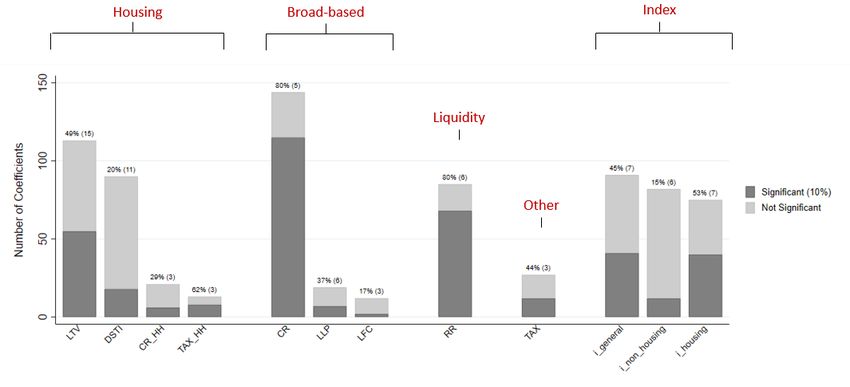
6

Moessner, 2018) and (Gambacorta and Murcia, 2019). This is represented by step 1 and 2 in
Figure 1. The second method relied on Google Scholar’s search engine using "effectiveness
of macroprudential policies" as keywords and focused on the empirical papers among the first
100 hits, which is illustrated by step 3 in Figure 1 .5

                                     Figure 1. Paper Selection Criteria

The third method consisted in snowballing and encompassed collecting all empirical papers
from the references of all studies identified in steps 1-3. This was followed by all empirical
papers from the new empirical papers’ reference list, and so on. The iteration stopped when
no new empirical papers were identified (illustrated by step 4 in Figure 1). The final set of
papers in the database (step 6) excludes 8 papers that appeared under multiple methods (step
5), and is broadly balanced between published and unpublished papers. Appendix Table A12
shows the final list of papers in the database. The three methods complemented each other.
The second method allowed capturing recent papers, while the other two helped identified
additional papers on specific tools, which may not have used the term "macroprudential"
in the text. The paper selection approach is similar to Havranek and Sokolova (2020) and
Havranek and Irsova (2011) who also use Google Scholar and cross-referencing.6

                                 B. Estimates and Statistics Selection

The collection of results within the selected papers included all estimated β̂ coefficients to
reduce the risk of introducing arbitrariness in the selection rule. Such an approach is also
followed by other meta-analyses in the literature (Cipollina and Salvatici, 2010; Disdier and
5 Google  Scholar searches throughout the entire text of the studies, not just the title and abstract. Using other
keywords such as "effect/impact of macroprudential policies" and other databases such as IDEAS/RePEC
databases did not yield more papers than the baseline search.
 6 Havranek and Sokolova (2020) cover 144 papers and about 3,000 results, compared to 58 papers and over

6,000 estimates in this paper.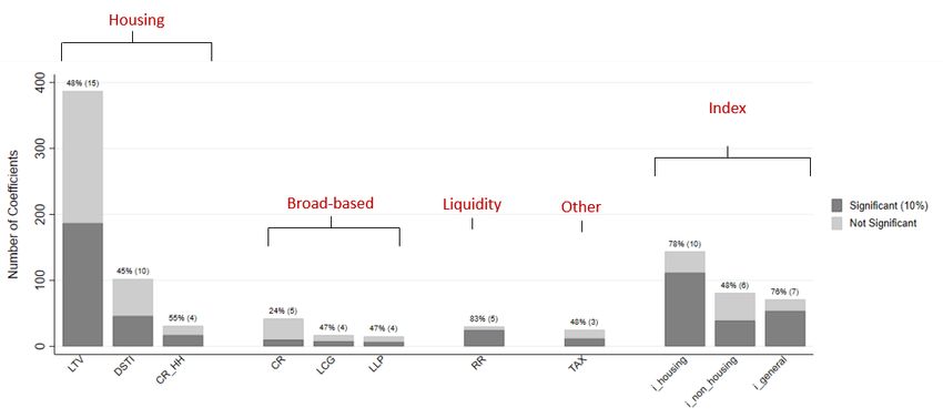
7

Head, 2008; Doucouliagos and Stanley, 2009; Havranek and Irsova, 2011).7 One exception
to the rule is the exclusion of estimates from specifications with interactions between MPM’s
and other variables. To include this information, a necessary input is a statistical test (and its
standard error) of the linear combination of the MPM coefficient and the interacted one, eval-
uated at some value of the interacted variable. No paper reported this test. Results presented
only in charts were requested from the authors and included in the database if provided by the
authors.

The collection of results included the coefficient β̂ , its standard error, the type of MPM tool
and how it was measured, the outcome variable, the estimation methodology, the unit of ana-
lysis (e.g. macro or micro level), sample characteristics (e.g. EM countries or all), whether the
specification corresponded to the most complete one in the paper, and the journal of publica-
tion if any.

                        C. MPM’s and Outcome Variables Classification

Given the lack of an universally accepted taxonomy of MPM tools, the classification of
MPM measures relied on the IMF’s Integrated Macroprudential Policy Database (iMaPP)
as a benchmark taxonomy. 8 The taxonomy includes 17 categories (e.g. capital requirement,
loan restrictions) and 4 classes of subcategories (e.g. household, corporate, broad-based and
FX targeted measures).9 This approach helped increase the comparability of tools across stud-
ies. The database also provides a mapping of these individual tools into broader groups, using
the classification in IMF (2014): (i) Broad-based tools which include counter-cyclical capital
buffers, conservation buffers, capital requirements, leverage limits, loan loss provisions, limits
on credit growth, loan restrictions and limits on foreign currency loans; (ii) Liquidity tools
which include liquidity coverage ratios, limits on loan-to-deposit ratio, limits on FX positions,
and reserve requirements; (iii) Housing tools which include housing sector specific measures
such as limits to loan-to-value ratios, limits to debt-service-to-income ratio, loan restrictions,
and other sector-specific capital requirements, loan loss provisions, and taxes and levies; (iv)
Other tools which include measures on systemically important financial institutions, taxes and
levies, and other measures.10 Appendix Table A1 provides details on the individual macropru-
dential tools, relying mainly on the description provided in the iMaPP, along with how they
map into the groups of measures described above.
7 Section    IV.A addresses also concerns related to quality of estimates within and across papers, since Andrews
and Kasy (2019) note that some estimates may correspond to inferior specifications.
 8 The iMaPP is a comprehensive macroprudential policy database in terms of instruments, countries, and time

periods combining information from five existing databases, as well as the IMF’s Annual Macroprudential
Policy Survey, and various additional sources (see Alam and others, 2019, for details).
 9 If a paper reports a measure belonging to one of the categories (e.g. loan loss provision (LLP)) and subcate-

gories (e.g. household (HH)), it was recorded as such, even if it implied adding an MCM category. For example,
the iMapp does not report the classification LLP_HH. On the other hand, not all iMapp categories were used if
there were no papers on those tools, for example the breakdown of limits on credit growth (LCG) into household
(HH) and corporate (CORP) sectors. As a result, the total number of categories and subcategories used in the
database is 33 while the iMapp includes 27.
10 If there is no information on whether the measure is targeted, it is classified as broad-based.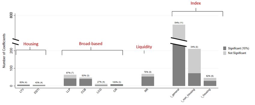
8

Finally, for parsimony, the database groups the dependent/outcome variables according to
10 categories: balance sheet fragility, bank default risk, capital flows, corporate credit, credit,
house price, household credit, economic activity, non-bank credit and other outcomes. The
Appendix Table A2 shows a description of the relevant outcome variables included in each of
these categories.

                                   D. MPM’s Measurement

The way MPM 0 s are measured in the literature can be grouped into three types. The first
group, corresponding largely to the first wave of studies measures the impact of macropruden-
tial tools based on the cross-country variations in policy settings (e.g. Cerutti, Claessens, and
Laeven, 2017; Claessens, Ghosh, and Mihet, 2013; Lim and others, 2011). Typically, stud-
ies of this sort define MPMs as a set of dummies that take the value one during the years in
which the instrument was used and/or in place in a country and zero otherwise.

A second, more predominant strand of literature relies on the direction of change of the policy
stance to identify impacts. Here, MPM is typically a discrete variable taking the values -1, 0,
and 1, indicating episodes of loosening, neutral, and tightening actions, respectively (Kuttner
and Shim, 2016, and many others). Within this set of papers, the bulk of the evidence comes
from tightening episodes with fewer papers exploring loosening actions.

Finally, few and more recent studies measure MPM’s with attention to the intensive margin.
Examples include Jiménez and others (2017) who studied the effects of the Spanish dynamic
provisioning mechanism and Richter, Schularick, and Shim (2019) who used a narrative
identification strategy to measure the intensity of LTV changes.

Often times, papers use a composite measure of MPM’s. For example, Kuttner and Shim
(2016), Cerutti, Claessens, and Laeven (2017), Claessens, Ghosh, and Mihet (2013) look at
borrower targeted measures and construct a composite of LTV and DSTI limits, and Akinci
and Olmstead-Rumsey (2018) and Vandenbussche, Vogel, and Detragiache (2015) construct
a composite MPM measures based on broad-based, liquidity, housing and other measures.
All composite MPM measures are also categorized into: (i) housing, (ii) non-housing (broad-
based, liquidity and other), and (iii) general, which includes both housing and non-housing
measures.

                                      E. Standardization

The literature does not have a standard definition of the variables used to measure the effects
of macroprudential policy. Therefore, they vary widely in terms of economic meaning (e.g.
house prices, credit), their measurement (e.g. log-levels, real or nominal growth rates, ratios,
etc.), the time horizon of the analysis (e.g. over one quarter, one year), or their underlying
9
distribution (e.g. micro data vs. macro data, or EM countries vs. advanced). Enhancing com-
parability of effects across studies requires normalizing the β̂ coefficients and their standard
errors by the standard deviation of the corresponding outcome variable.11
Where MPM’s are measured discretely (either as a dummy variable indicating whether a pol-
icy is in place or in terms of a change to tightening or loosening), the effect size is interpreted
as a standard deviation change to the outcome variable in response to a change in the policy
either in the direction of tightening or adoption of the tool.
When the MPM’s are measured considering the intensive margin, the effect is still standard-
ized using the standard deviation of the outcome variable, but the database includes also the
standard deviation of the MPM change when available. In this case, the effect size is inter-
preted as a standard deviation change to the outcome variable in response to unit change in
the policy variable, which in most cases corresponds to a one percentage point change in the
corresponding tool.
When available, the standardization approach used the summary statistics specific to the
sample that produced the selected β̂ coefficient. Regression-specific summary statistics were
requested from the authors if not available in the paper. If not provided, the standardization
used the summary statistics available in the paper for the specific outcome variable consid-
ered.
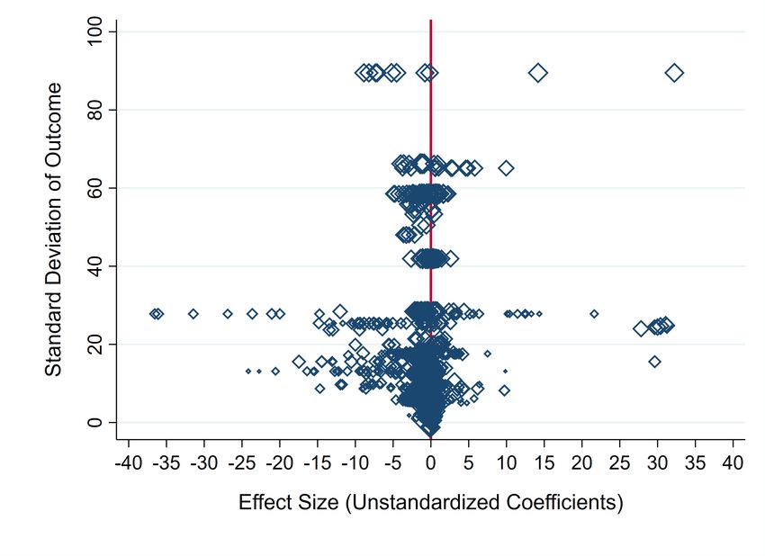
Figure 2. Effect Sizes
(a) Raw Effects and Outcome Standard Deviation (b) Distribution of Standardized Effects
Note: Each diamond in the figure represents a coefficient; size is proportional to its precision.
11 Yuan and Chan (2011) show that dividing the standard error by the outcome’s standard deviation is a good
approximation of the standardized standard error and under certain conditions, it is close to being consistent
in the case of multiple regressions. See also Nieminen and others (2013) and Peterson and Brown (2005) for a
similar approach.10
Figure 2a shows that the range of unstandardized effects is wide and dispersed, which may
be explained by the aforementioned heterogeneity in outcome variables but also in MPM
tools in our dataset. In contrast, Figure 2b shows that once coefficients are standardized, the
distribution is approximately normal, allowing us to draw comparisons more easily, with
effect sizes concentrated in the 0 to -0.2 standard-deviations region.
Our standardization procedure ensures that all effects can be comparable and interpreted
similarly, regardless of how the outcome variables are measured, the time-horizon over which
they are measured, the unit of analysis, or the sample. The importance of the standardization
of coefficients in enhancing comparability of results can be visually inferred through Figure 2
which plots the distribution of raw and standardized effects.
III. D ESCRIPTIVE S TATISTICS
A. Database Overview
Figure 3. Focus of Studies: MPMs and Outcome Variables
Figure 3, provides a broad overview of all instruments and outcome variables studied in the
papers in our database. Each cell includes the number of papers studying the effect of an11 MPM tool (shown on the first column) on an outcome variable (shown on the top row). The darker shade indicates an increased number of papers associated with that pair. The upper left corner of the matrix concentrates the most widely studied pairs, notably those related to the housing sector such as borrower-based housing measures and their impact on house prices and household credit. The first row of the matrix groups studies where macroprudential policy is measured as a composite index of multiple tools. Most studies examine economy-wide impacts using typically cross-country datasets, but a growing number of studies exploit also the availability of micro-level data to assess the ef- fects of macroprudential policy. For example, Jiménez and others (2017) use bank-firm-level data on loans from the Spanish credit registry to study the effects of dynamic provisioning on bank credit provision and other outcome variables. Overall, 43 percent of studies are cross- country using macro-level data, 10 percent of studies are cross-country using micro-level data, 12 percent of studies are country studies using macro-level data and 34 percent of studies are country studies using micro-level data. The set of control variables used also varies and typically include other MPM’s (61 percent of results), interest rates (77 percent of results), other macroeconomic variables (61 percent of results), cross-sectional fixed effects (80 percent of results), and time fixed effects (35 percent of results). There is also significant variation across papers in their empirical approaches, in particular with regards to dealing with the endogeneity of macroprudential policy actions. Many of the studies use panel-data techniques and deal with reverse causality concerns through timing assumptions and focus on the lagged effect of macroprudential policy changes (e.g. Richter, Schularick, and Shim, 2019). A few other studies use GMM or instrumental variables (e.g. Cizel and others, 2019; Zhang and Zoli, 2016), instrumenting macroprudential policy with the vector of exogenous covariates. Several other studies, typically using micro-level data make use of an event-study or difference in difference methodology to identify the effects of macroprudential policy often looking specifically at entities around the binding constraint or applicability thresholds (e.g. Aiyar, Calomiris, and Wieladek, 2014; Jiménez and others, 2017). 12 Most studies focus on effects of up to a year, but some use VAR’s (e.g. Carreras, Davis, and Piggott, 2018) or local projection methods (Richter, Schularick, and Shim, 2019) to under- stand the effects of macroprudential policy at various horizons, but also to allow the exoge- nous covariates to be inter-related (e.g. Kim and Mehrotra (2018)). 13 12 Overall, half of the studies present at least one result using OLS estimation, one quarter of the studies present at least one result using GMM estimation, 15 percent of the studies present at least one result using difference-in- difference estimation while half of the papers present at least one result based on some other method (e.g. Panel VAR, Quantile Regression, etc). 13 Nearly all papers present results for horizons of up to one year while one quarter of studies also present results for over one-year horizons.
12

                                       B. Statistical Significance

This subsection presents a first cut of the database focusing on statistical significance. Macro-
prudential tools are grouped into the four types described in Section II: (i) Broad-based tools;
(ii) Liquidity tools; (iii) Housing tools; and (iv) Other tools.

Figure 4 shows the number of statistically significant coefficients, at least at the 10 percent
level, and the total number of coefficients on the vertical axis and the analyzed MPM tool on
the X-axis. The figure focuses on the three most widely studied outcome variables: household
credit (panel a), house prices (panel b), and total credit (panel c) displaying about half of the
6627 coefficients in our database. The sample includes coefficients estimated using all types
of policy change measurement, for tightening and loosening episodes, for all time horizons,
and whether or not statistics could be collected for standardization. At the top of each bar,
the figure shows the percent of significant results and the number of papers, in parenthesis,
from which these coefficients were collected. Consistent with Figure 3, Figure 4 shows that
limits on loan-to-value ratio and on debt-service-to-income ratio stand out as the most studied
measures, when looking at household credit or house prices as outcome variables. But the
coefficients are not always statistically significant. And this pattern seems to hold for individ-
ual MPP measures or composite ones. Finally, turning to total credit growth, measures such
as loan loss provision, reserve requirements and composite measures seem to be the more
widely studied, with also a large fraction of statistically significant coefficients. In sum, a very
heterogeneous picture which makes it difficult to extract a clear common ground. To make
progress, meta-analysis techniques come in handy by allowing summarizing these findings to
extract a bottom line.

                                              C. Magnitudes

Table 1 presents summary statistics of standardized effects for the broad outcome buckets
described in Section II. For the statistics to be comparable, only results that could be standard-
ized and that measure effects for a horizon of up to one year (henceforth short-term horizon)
are used to produce the table. These filters imply that Table 1 summarizes approximately 50
percent of all coefficients in the database.14

14 Approximately  60 percent of the results in the database correspond to effects within a one-year horizon, but
in constructing Table 1 about 10 percent of results are lost due to the lack of summary statistics to normalize
coefficients.
13
Figure 4. Fraction of Coefficients Statistically Significant at 10% level or higher
(a) MPM Effects on Household Credit
(b) MPM Effects on Housing Prices
(c) MPM Effects on Credit
The The numbers on top of each bar are the percentage of significant results and (in parenthesis) the number of papers. The
"i_general" bar in chart (c) is not shown in full,the total number of coefficients for "i_general" index on the outcome category "credit"
is 696. Details of each MPP tools and outcome categories can be found in Table A1 and Table A2, respectively.14
Table 1. Summary of Standardized Macroprudential Policy Effects
Obs. Mean Std. Min Max
Dev.
MPM in place (0,1):
Balance sheet fragility 249 -0.02 0.09 -0.94 0.21
Capital inflow 78 0.05 0.19 -0.83 0.77
Corporate credit 51 -0.01 0.54 -1.69 2.24
Credit 190 -0.38 0.71 -3.52 1.90
Economic activity 30 0.13 0.55 -1.67 0.95
House price 157 -0.09 0.39 -2.06 1.19
Household credit 176 -0.15 0.29 -1.23 0.93
All Outcomes 931 -0.12 0.44 -3.52 2.24
MPM change (-1,0,1 in the direction of tightening:)
Balance sheet fragility 5 -0.02 0.03 -0.05 0.01
Bank default risk 38 -0.31 0.62 -3.35 0.40
Capital inflow 116 0.00 0.10 -0.37 0.34
Corporate credit 37 0.08 0.07 -0.11 0.34
Credit 168 -0.07 0.45 -2.21 2.40
Economic activity 392 -0.08 0.51 -5.36 1.57
House price 353 -0.01 0.31 -1.44 2.69
Household credit 411 -0.14 0.32 -1.59 1.02
Non bank credit 18 0.02 0.04 -0.01 0.14
All Outcomes 1538 -0.07 0.38 -5.36 2.68
MPM intensity (level or change in levels):
Balance sheet fragility 14 -0.25 0.23 -0.66 -0.01
Credit 55 -1.21 1.14 -5.91 -0.06
Economic activity 150 0.00 0.01 -0.04 0.05
House price 238 -0.28 0.20 -0.94 0.40
Household credit 168 0.01 0.04 -0.22 0.20
All Outcomes 625 -0.21 0.50 -5.91 0.40
The table reports the summary statistics for standardized macroprudential policy effects for each outcome category by
different types of macroprudential policy measurements. The signs of effects for some outcomes have been reversed to
fit the direction of the overall outcome category; see Appendix Table A2 provides details on the outcomes within each
categorization and the sign transformations. It should be noted that the summary statistics bundle together the effects
of all types of macroprudential instruments. The sign is reversed for loosening only episodes for ease of interpretation.
The summary stats are presented separately by the way in which macroprudential policy is
measured. The first panel summarizes the effects of the availability of macroprudential tools
on the corresponding outcomes, which comprises 30 percent of the short-term horizon results15
in our database; the summary statistics in this cell, therefore represent the standard deviation
change in the outcome variable from having the macroprudential policy in place. The second
panel shows outcomes from studies that measure adjustments in the tool through -1, 0, and
1, dummies indicating policy episodes of loosening, no change, and tightening, respectively,
and comprises 50 percent of the short-term horizon results; the summary statistics in this cell,
therefore represent the standard deviation change in the outcome variable from changing the
macroprudential policy, in the direction of tightening. The third panel includes outcomes from
papers using either the actual value of the tool (e.g. reserve requirements) or some transfor-
mation of it (e.g. a step function of LTV limits) that considers intensity of use; the summary
statistics in this cell, therefore represent the standard deviation change in the outcome vari-
able from a unit change in the intensity of macroprudential policy use.
Taking up first the case of results in the first panel, it can be seen that effects encompass both
positive and negative values across all outcomes. As noted before, the results are concentrated
around measuring effects on credit (including household credit) and house prices. The effects
reported for several outcome variables are highly variable, with the standard deviations most
exceeding the mean.
A similar pattern was found for the second set of results which measure discrete macropru-
dential policy changes in the direction of tightening. In this set, the results are similarly fo-
cused on examining credit and housing outcomes. For the third set of results, which include
information on intensity in the change of macroprudential policy, there are fewer outcomes as
there are also fewer papers. They focus on credit (including household credit), house prices
and indicators of economic activity (e.g. real GDP growth, employment, and firms sales).
The distribution of effect sizes in this set are not easily comparable, because the actual level
or change of macroprudential policy varies substantially across studies and the coefficients
(effect sizes) are not estimated as elasticities. Nonetheless, both negative and positive effects
are reported.
Finally, Appendix Table A11 provides a more dissagregated version of Table 1 by breaking
down the summary statistics by sectoral MPM measures.
D. Symmetry
As noted in Table 1, the bulk of our database includes papers looking at changes in macro-
prudential policy in the direction of tightening or loosening. But these effects need not be
the same in absolute value. The rationale for the possibility of asymmetric effects lies in
that tightening measures are generally employed in expansionary phases of the cycle, when
incentives to leverage up can be stronger than in the correction phase. In this context, intro-
ducing macro-prudential measures are more likely to impose binding constraints. Loosening
measures, on the other hand, tend to be implemented during the correction phase, with the
intention of releasing buffers and provide a boost to agents’ borrowing capacity. However, it
is not necessarily the case that agents can or would want to take advantage of it, for example16
due to a reduction in income or increased uncertainty.15 The presence of leakages can also
influence symmetry of effects if the incentives to circumvent regulation are stronger in the
buildup phase of the financial cycle, when constraints bind.
About sixty percent of the studies in our database discuss effects of either tightening or loos-
ening macro-prudential policies, with examples including McDonald (2015), Kuttner and
Shim (2016), Jiménez and others (2017), and Richter, Schularick, and Shim (2019). However,
more than a quarter of these papers study only tightening actions, a few (4) of them study eas-
ing actions alone, and about 20 percent of them study both. Overall, there is more evidence
about the effects of tightening than loosening macro-prudential policies, largely by virtue of
the developments in the past decade which constitute the largest parts of the samples. A large
proportion of these findings pertains to housing market tools.
Overall, the estimated effects of tightening are more often statistically significant than those
of loosening (see Figure 5, left-hand-side chart).16 Among papers looking at the effects of
tightening and/or loosening, 46 percent of results find tightening coefficients to be statistically
significantly different from zero at the 10 percent level, versus 36 percent for easing actions.
When restricting the analysis to within paper comparisons, that is, looking only at the 13
papers analyzing both tightening and loosening effects in comparable regressions (i.e. same
specification, tools, and sample), tightening coefficients are significant in 61 percent of cases,
and easing coefficients in only 37 percent of them (see Figure 5, right-hand-side chart).
Figure 5. Results on Asymmetries
15 Increased uncertainty about economic outcomes during the correction phase can intensify a precautionary
motive under which agents become "too cautious" and may wish to reduce leverage.
16 The figure focuses only on statistical significance of tightening/easing coefficients without differentiating tools
or outcome variables.17
These results largely mirror the conclusions from papers looking at the effects during differ-
ent phases of the financial cycle.17 More specifically, macroprudential measures employed
during the expansionary phase are statistically significant at the 10 percent level in 70 percent
of cases (and 65 percent of the results which directly compare boom and bust periods). At the
same time, measures implemented during the correction phase, are statistically significant in
56 percent of cases.
Figure 6. Result on Asymmetries between Tightening and Easing
Turning to magnitudes, and fixing the sample on those 13 papers studying both directions18
Figure 6 shows a direct comparison (in absolute value) of tightening and easing coefficients.
In general, the figure shows that there is more mass above the 45-degree line, suggesting
that the magnitude of tightening coefficients tends to be more often than not larger than the
comparable easing coefficient. More specifically, we find that in about 57 percent of cases,
the estimated coefficients for tightening measures are larger in absolute value than those
for easing. Moreover, when restricting our attention to the tightening coefficients which are
statistically significant and negative (about 40 percent), they overwhelmingly exceed the
17 The financial cycle is defined somewhat differently in each paper in terms of the specific metric or method-
ology to identify the cyclical position, for simplicity these phases are refered to as "expansionary" and "cor-
rection." Examples include Claessens, Ghosh, and Mihet (2013), Lim and others (2011), McDonald (2015),
Vandenbussche, Vogel, and Detragiache (2015).
18 For this analysis we also include non-standardized results in our database to cover a broader sample. Since we
are making comparisons within papers, standardization becomes less critical.18
effects of easing actions. But it is important to note that in about 20 percent of cases, the
effects of easing are either stronger than tightening (e.g. Barroso, Gonzalez, and Doornik,
2017, on reserve requirements) or the two are too close to make a call.
In general, the evidence suggests that the effect of tightening has a larger quantitative impact
and is more often statistically significant than the effect of easing. Beyond any economic
rationale for these results, there is also a statistical reason which is that the larger number of
observations for tightening actions allows more power in identifying their effects.
IV. M ETA -R EGRESSIONS
A. Methodology
The previous section illustrated significant variation in the statistical significance and mag-
nitude of coefficients. However, extracting a summary view requires combining information
about precision and magnitudes of estimates to arrive at an "average" effect. To this end, this
paper uses a meta-analysis framework to quantitatively synthesize estimated effects and ulti-
mately examine how they vary with some studies or results characteristics.
Figure 7. Forest Plots: Effects of Tightening Macroprudential Tools on Credit
To illustrate how a meta-analysis works, let us assume that the standardized true average ef-
fect of macroprudential policy on credit is denoted by β . The database includes the estimated19
effect size for result j from the kth study, β̂ jk ∼ N(β , σ 2jk ),19 which incorporates some error
around the true effect (typically from sampling variability) with variance given by σ 2jk . This
variance of the estimated effect is given by the square of the effect’s standard error, which is
included in the database. The meta-analysis framework then allows us to recover β by tak-
ing a weighted average of β̂ jk across studies, with the weights inversely proportional to the
standard error of each estimated effect, implicitly giving higher weights to more precise re-
sults as is typically done in meta-analyses (e.g. Bruns, 2017; Sutton and Higgins, 2008). As
an illustration, Figure 7 shows the elements of the meta-analysis described above - the esti-
mated effects sizes, its variance, and our measure of the true average effect - focusing on the
short-term effects for credit from tightening macroprudential policies (without differentiating
tools for now). Each row of this figure plots the standardized effect from each of the studies
together with its 95th percent confidence intervals. The vertical red line shows the precision
weighted average of these effects, while the black line shows the simple average of all the
effects. As shown in the figure, there is substantial heterogeneity in the precision of estimates,
with the distribution of effects slightly negatively skewed, as expected.
In estimating average effects, however, the β above is likely to differ across tools, outcome
variables, and other determinants. In what follows, this heterogeneity is exploited through a
meta-regression, which includes covariates that help explain how the true effects may vary
(Greenland, 1987). The meta-regression framework is thus given by:
β̂ jk = ∑ θm · MPM mjk + γX jk + δ · SE 2 (β jt ) + ε jk (1)
m
where β̂ jk corresponds to some outcome variable of interest and is regressed on a set of dum-
mies, MPM mjk , each taking the value of 1 when the effect corresponds to MPM measure m,
which could be category of tools (e.g. broad based) or an specific tool (e.g. LTV limits).
Therefore, the coefficients θm denote the average effect of MPM m, on the outcome variable
in question, controlling for attributes of the estimate β̂ jk collected in X jk . These attributes in-
clude a dummy variable to identify estimates taken from papers published in a peer-reviewed
journal and a dummy variable that identifies estimates taken from the most complete specifi-
cation within a study. The inclusion of the latter variable is motivated by the possibility that
inferior specifications could bias our average effects.20 Finally, the term SE 2 (β jt ) is a publi-
cation bias selection correction based on the standard error of β̂ jk , in line with the standard
practice in the meta-analysis literature.
The publication bias may arise if researchers select their results based either on its statistical
significance or on a prior expected direction of the effects (Havranek, 2015). As proposed by
19 The assumption that all effect sizes are the the same and equal to the true effect size average effect, β , is
typically referred to as the common-effect meta-analysis model, as suggested by Rice, Higgins, and Lumley
(2018).
20 An alternative would have been to identify estimates taken from a best-practice regression specification in the
literature (Bruns, 2017), but lacking such benchmark, as mentioned in Section II, this issue is instead addressed
by identifying estimates from regressions that have the most exhaustive set of controls, within each study.20
Stanley and Doucouliagos (2014),21 This selection bias problem is addressed by including
as control the square of the estimate’s standard error, SE 2 (β jt ). Appendix V II shows that
the bias is significant even among published paper, but considerably smaller and statistically
insignificant in micro-based studies.
The sample for the meta-regressions comprises all effects estimated within the one-year hori-
zon i.e., short-term effects and excludes results that could not be standardized. The sample
also excludes a very small fraction of outliers, those effects that exceed -3 or +3 standard
deviation, when the MPP is analyzed in terms of existence or changes. Note that the error in
equation (1), ε jk ∼ N(0, σ 2jk ), is heteroskedatic, with the degree of heteroskedasticity given by
the estimate’s standard error. This is accounted for by using a weighted least squares estima-
tion procedure with the inverse of standard errors as weights, which yields efficient estimates.
B. Baseline Results
Table 2 reports the baseline results from estimating equation (1) focusing on the short-term
effects of MPP changes (in the direction of tightening) on credit, including household credit.
The sample comprises the results where the change of macroprudential policy (most typically
tightening episodes) through -1,0,1 dummies, as described in Section II.22 The sample ex-
cludes results from (i) loosening actions to ensure a comparable interpretation of the effects,
although these are still few; and (ii) MPM indices, which combine instruments across differ-
ent categories to ensure that the MPM categories in the regressions are mutually exclusive,
but provide separately results on these later in this section. The classification of macropruden-
tial tools follow the broad categories described in Section II.
Column (1) reports results from a simple specification without adding any controls and shows
that liquidity and other tools tend to have relatively larger effects, when tightened, on total
credit. On average, a tightening of these tools is associated with a 0.12 standard deviation
reduction in total credit compared to the 0.04 standard deviation effect on reducing credit ob-
tained from tightening housing and broad-based tools. Liquidity and other tools are bundled
together because of the fewer observations on the latter but Table 3 show their effects sep-
arately. One caveat to note is that a comparison of average effect sizes across the different
categories of macroprudential policies or even tools within a category, is valid to the extent
21 Stanley and Doucouliagos (2014) show that in the presence of a selection bias, the reported effects may be
regarded as incidentally truncated (the truncation is based on the z-value or t-value of the coefficient). They
show that including the square of the estimate’s standard error as a control performs well in reducing the bias.
Andrews and Kasy (2019) propose bias-corrected estimators based on (non-parametrically) identifying the
conditional selection-related publication probabilities up to scale. While the regressions in the main text rely
mainly on the correction proposed by Stanley and Doucouliagos (2014), the appendix also shows results based
on the selection correction procedure outlined by Andrews and Kasy (2019).
22 The sample consists of non-cumulative effects up to one year. For studies that reported only cumulative effects,
the per-period effect was backed out by dividing the former by the corresponding horizon in order to standardize
coefficients. This step was necessary as summary statistics typically corresponded to the one-period effect. Over
80 percent of the results in the sample correspond to quarterly frequency and the rest to monthly frequency.21
that the average tightening of macroprudential tools in the corresponding sample is approx-
imately equivalent, which does not need to be the case. In other words, the stronger impact
from liquidity tools may just be driven by much more intense tightening of these tools com-
pared to others. This caveat applies to the literature in general as most studies do not measure
the intensive margin in the use of macroprudential tools.23
Table 2. Average Effects of Tightening Macroprudential Tools on Credit
Dep. Var.- Standardized effects on Credit
(1) (2) (3) (4) (5)
Broad based -0.045∗∗∗ -0.037∗∗∗ -0.037∗∗∗ -0.053 -0.056∗∗∗
(0.002) (0.010) (0.010) (0.034) (0.007)
Housing -0.041∗∗∗ -0.051∗∗∗ -0.050∗∗∗ -0.058∗∗ -0.045∗∗∗
(0.007) (0.012) (0.012) (0.026) (0.011)
Liquidity & Other -0.118∗∗∗ -0.118∗∗∗ -0.118∗∗∗ -0.135∗∗∗ -0.129∗∗∗
(0.005) (0.005) (0.005) (0.030) (0.009)
SE sq. (Pub. Bias Correction) -0.780 -0.759 -2.314∗∗
(1.268) (1.281) (0.837)
Specification with incomplete controls 0.013 0.024∗∗∗
(0.015) (0.008)
Non-Published Papers 0.011
(0.026)
Study over-weighting adjustment X X X
Journal quality weighting X
Observations 438 438 438 438 438
r2 0.695 0.607 0.608 0.613 0.704
The table reports the average effects of tightening macroprudential measures on credit (including credit to households) . All columns report re-
sults from a weighted least squares specification where the weights are proportional to the precision of each result. Columns (2)-(3) additionally
apply weights proportional to the number of results observed per study to avoid for any one study to drive the results. To account for possible
dependence across results/observations for the same study, standard errors are clustered at the study level and reported in parentheses. *
indicates significance at 10%; ** at 5%; *** at 1%.
23 As described in Section III.C, a few studies in the database do consider the intensity of use of macroprudential
tools, not just the direction of change, but are too few to be summarized through metaregressions.22
Accounting for result quality and robustness checks: Columns (2)-(4) successively check
for the robustness of these results with a view also to control for the varying quality of results
and papers, to find that the pattern and magnitude of the baseline results remains largely
unchanged:
• First, some studies report many more results than others and therefore the regressions
in Columns (2)-(4) use sampling weights proportional to the inverse of the number
of estimates reported by each study. The results are not overly influenced by a single
study.
• Second, Columns (3)-(5) show the results after adding the selection bias correction
term as explained in the previous subsection. Even though the selection term is statisti-
cally significant in Column 5, the overall pattern of results are only slightly affected by
it.
• Third, two dummy variables were added to control for results coming from unpub-
lished papers (Column 4) and from specifications which are not the most complete
ones within a paper (Columns 4 and 5), which allows controlling for quality of papers
and results. The rationale behind the publication dummy is that the refereeing process
would help ensure the proper use of estimation methodology, calculation of standard
errors, and other quality control elements; whereas the incomplete specification dummy
would control for quality of specifications within a paper. Both dummies are set up
such that the baseline results correspond to the average effects among published papers
and among the most complete specifications within papers.24 The results are robust to
the inclusion of these controls, although the effect on broad-based tools loses precision.
• Fourth, to account more comprehensively for paper quality, the regression in Column
(5) introduces an additional weighting scheme that ranks papers according to the jour-
nal where they are published. 25 The magnitude of the average effects continues to be
robust and stable with the broad-based measure now regaining its precision.
• Finally, Appendix Table A6 shows that the results presented in Table 2 are also robust
to dropping observations where standardized effects were calculated using imputed
summary statistics, and to sequentially excluding a specific study from the analysis.
Results from other MPM measurements: As a third of the database also consists of results
from studies that measure whether the macroprudential policy is in place or not, Appendix
24 While some meta-analysis studies include only published papers, the inclusion of unpublished papers follows
from the relatively young age of the research on macroprudential policy effects.
25 The weighting assigns a value of 4 to ‘world-leading’ journals, 3 for ‘internationally excellent’, 2 for ‘recog-
nised internationally’ and 1 for other journals. The categorization of journals into the ranks 4-2 is obtained from
Hole (2017), the most recent list (incorporating the relatively new American Economic Association and Econo-
metric Society journals) that has been published in a peer-reviewed journal. All non-published papers were
assigned a value of 0.5, thereby ranking them the lowest but still included in the regression. The specification
for Column (5) excludes the weighting for study over-adjustment for simplicity, but the results are stable to its
exclusion.23
Table A4 reports average effects from these studies. The table shows an effect of 0.2, 0.1
and 0.09 standard deviation reduction in credit from having broad-based, housing sector,
and liquidity/other tools respectively. These average effects are relatively larger than those
reported in Table 2, which may possibly be capturing cumulative effects of several tightening
actions over time. An alternative explanation is that they may simply reflect differences in
economic circumstances across countries since these studies mainly exploit cross-country
variation in the toolkit.
C. Heterogeneity of Average Effects
The next results explore how the average effects vary, looking first at the effects of individual
instruments, followed by examining the effects on two additional outcome variables: house-
hold credit and house prices. Table 3 shows the average effects for the most widely studied
instruments in the literature as identified in Section II.C. The average effect across all other
tools is captured by the “other MPP” variable.
Tighter limits to LTV and DSTI are found to have similar impacts on total credit or house-
hold credit, reducing both by about 0.05-0.065 standard deviations, but their average effect
on house prices is statistically insignificant. Liquidity tools - mainly reserve requirements
and limits to the net FX open position- have relatively larger effects on credit as before. How-
ever, loan loss provisioning is statistically insignificant across the three outcome variables.
Capital requirements26 appear to affect total credit and house prices, but their average effect
on household credit is less precise. On the other hand, tightening loan-loss provisions has
a statistically insignificant effect on all outcomes, but the coefficient is of the order of 0.03
standard deviations.
Next, effects are disaggregated by country setting and examined whether the effects of macro-
prudential policy are different in emerging market economies. This is done by sub-sampling
results based exclusively on emerging market countries (EM); and samples consisting of ad-
vanced, emerging, and low-income countries or exclusively advanced countries (Mixed), with
results shown in Columns (1) and (2) of Table 427 which shows evidence of relatively larger
average effects in EM’s for housing and liquidity (and other) measures. However, the reported
results for emerging markets have wider confidence intervals.
26 Inthis specification, capital requirements includes sectoral capital requirements (such as capital requirements
on housing sector credit).
27 Table 4 omits the control variable for non-published papers because of the very few published (at most two) in
the EM vs. Mixed split sample. For robustness, Appendix Table A10 presents results slightly differently, with
the micro vs macro split including the publication dummy, where it is feasible to include because of enough
published papers. The conclusions are similar to those in Table 4.You can also read