User-oriented hydrological indices for early warning systems with validation using post-event surveys: flood case studies in the Central Apennine ...
←
→
Page content transcription
If your browser does not render page correctly, please read the page content below
Hydrol. Earth Syst. Sci., 25, 1969–1992, 2021
https://doi.org/10.5194/hess-25-1969-2021
© Author(s) 2021. This work is distributed under
the Creative Commons Attribution 4.0 License.

User-oriented hydrological indices for early warning systems with
validation using post-event surveys: flood case studies in the Central
Apennine District
Annalina Lombardi1 , Valentina Colaiuda1,2 , Marco Verdecchia2 , and Barbara Tomassetti1
1 Center   of Excellence, University of L’Aquila, via Vetoio, 67100 Coppito (L’Aquila), Italy
2 Department    of Physical and Chemical Sciences, University of L’Aquila, via Vetoio, 67100 Coppito (L’Aquila), Italy

Correspondence: Annalina Lombardi (annalina.lombardi@univaq.it)

Received: 15 June 2020 – Discussion started: 31 July 2020
Revised: 4 December 2020 – Accepted: 2 March 2021 – Published: 14 April 2021

Abstract. Floods and flash floods are complex events, de-          1   Introduction
pending on weather dynamics, basin physiographical char-
acteristics, land use cover and water management. For this         Floods are recognized among the most destructive natural
reason, the prediction of such events usually deals with very      hazards (Berz et al., 2001), affecting 21 million people, glob-
accurate model tuning and validation, which is usually site-       ally, each year; unfortunately, this dramatic estimation is ex-
specific and based on climatological data, such as discharge       pected to rise up to 54 million by 2030 (Lehman, 2015). So
time series or flood databases. In this work, we developed         far, according to the data reported by MunichRe (2018), 2017
and tested two hydrological-stress indices for flood detection     has been the worst year in terms of overall loss caused by nat-
in the Italian Central Apennine District: a heterogeneous ge-      ural hazards.
ographical area, characterized by complex topography and              It has also been long recognized that the increase in the
medium-to-small catchment extension. The proposed indices          frequencies of severe precipitation events represents a char-
are threshold-based and developed considering operational          acteristic signature of observed climate changes at a global
requirements of National Civil Protection Department end-          scale; the intensification of the hydrological cycle due to the
users. They are calibrated and tested through the application      warming climate is projected to change river floods’ magni-
of signal theory, in order to overcome data scarcity over un-      tude and frequency (Field et al., 2012; Blöschl et al., 2017).
gauged areas, as well as incomplete discharge time series.         Kundzewicz and Schellnhuber (2004) highlighted that about
The validation has been carried out on a case study basis,         one-third of all reported events and one-third of economic
using flood reports from various sources of information, as        loss resulting from natural catastrophes are attributable to
well as hydrometric-level time series, which represent the         floods all over the world. Different works seek to analyse the
actual hydrological quantity monitored by Civil Protection         impact of climate change scenarios on flood hazards in Eu-
operators. Obtained results show that the overall accuracy of      rope, finding that several European countries will experience
flood prediction is greater than 0.8, with false alarm rates be-   increasing flood risk in the future (Dankers and Feyen, 2009;
low 0.5 and the probability of detection ranging from 0.51         Feyen et al., 2012). Alfieri et al. (2015) showed a significant
to 0.80. Moreover, the different nature of the proposed in-        increase in the frequency of extreme events (i.e. larger than
dices suggests their application in a complementary way, as        100 %) in 21 out of 37 European countries, in the reference
the index based on drained precipitation appears to be more        period 2006–2035, to be followed by a further deterioration
sensitive to rapid flood propagation in small tributaries, while   in the subsequent future. Blöschl et al. (2019) demonstrated
the discharge-based index is particularly responsive to main-      clear regional patterns of both increasing and decreasing river
channel dynamics.                                                  flood discharges in the past 5 decades in Europe, attributable
                                                                   to changing climate. More specifically, the Mediterranean
                                                                   area is one of the climate system’s hotspots most responsive

Published by Copernicus Publications on behalf of the European Geosciences Union.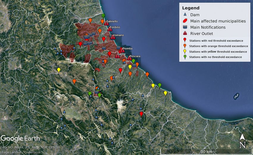
1970                                                    A. Lombardi et al.: Flood case studies in the Central Apennine District

to climate changes (Giorgi, 2006; Giorgi and Lionello, 2008).          roughness (Di Baldassarre and Montanari, 2009; Di Baldas-
Indeed, 185 flood events were recorded in the Mediterranean            sarre and Claps, 2011). Moreover, it is difficult to establish a
countries between 1990 and 2006, with the number of cases              flow discharge threshold value, beyond which the river can be
affecting Spain, Italy and France being 59 % of the total. On          considered under stress conditions; this value is site-specific
the Italian Peninsula, these events caused EUR 20 billion of           and refers to a certain river section and, therefore, cannot be
damage to buildings and infrastructures (Llasat et al., 2010).         considered general for the whole drainage network.
Mysiak et al. (2013) estimated that some 3.5 million people               In the IPCC (Intergovernmental Panel on Climate Change)
(6 % of the total Italian population) live in hydrogeological          SREX (Managing the Risks of Extreme Events and Disas-
risk areas. The history of Italy is characterized by many dev-         ters to Advance Climate Change Adaptation; https://archive.
astating floods, causing deaths, related economic loss, and            ipcc.ch/report/srex/, last access: 6 April 2021) report (Field
deep social and environmental impact. Given the high land-             et al., 2012), floods are defined as “the overflowing of the
scape variability, the complex topography and climatic vari-           normal confines of a stream or other body of water or the
ability, Italy is one of the most exposed countries to geo-            accumulation of water over areas that are not normally sub-
morphological risk. Meteorological patterns are frequently             merged. Floods include river (fluvial) floods, flash floods, ur-
characterized by deep convective clouds that originate in-             ban floods, pluvial floods, sewer floods, coastal floods, and
tense and localized rainfall, rapidly developing into localized        glacial lake outburst flood”. Precipitation intensity, duration,
floods. Salvati et al. (2018) estimated that 441 flood events          amount and timing are the principal mechanisms affecting
occurred over 420 Italian sites from 1965 to 2014, causing a           a flood event. Moreover, the relationship between the rain-
total number of 771 fatalities.                                        fall and drainage network response is complex (Bates et al.,
   Considering the last 2 decades, Italy is the 6th country in         2008; Kundzewicz, 2012) and sensitive to rain spatial dis-
the world for number of victims caused by hydrogeological              tribution. In large river basins, for example, river floods are
hazards and 18th in terms of economic loss (Eckstein et al.,           generated by intense and enduring rain, while short-duration,
2019). The European Parliament defined floods as “the po-              highly intense rainfall is expected to determine floods in
tential to cause fatalities, displacement of people, and dam-          small basins. Chen et al. (2010) have highlighted different
age to the environment, which can severely compromise eco-             flooding drivers. The main ones are (i) pluvial flood, due
nomic development”.                                                    to the limited capacity of a drainage system, and (ii) fluvial
   In the EU Directive 2007/60/CE concerning the “Assess-              flood, caused by deluges from the river channel. The fluvial
ment and management of flood risks”, the realization of a              flood events considerably differ from pluvial (rainfall) flood
flood risk map is prescribed over river basins with a signifi-         events in spatial–temporal scale including their magnitude.
cant potential risk of flooding (European Parliament, 2007).           The fluvial events usually occur for a duration of days or even
To this aim, tools for flood event prediction may also pro-            weeks with widespread damage in the floodplains of the river
vide useful information for the mitigation strategies during           system. On the other hand, pluvial flooding hardly ever hap-
the planning phase. Since the 1970s, the hydrological fore-            pens for more than a 1 d duration and with an influence on
cast has improved (e.g. Jain et al., 2018; Ranit and Durge,            local regions (Chen et al., 2010; Patra et al., 2016; Apel et
2018; Hapuarachchi et al., 2011); a comprehensive review of            al., 2016).
the different hydrological forecasting techniques is given in             In general, precipitation indices are applied for flash flood
Teng (2017), where empirical models are found to be suffi-             prediction, since a negligible contribution of infiltration pro-
ciently suitable for post-event monitoring and analysis, while         cesses is assumed for small catchments (Reed et al., 2007;
hydrodynamic models are better suited for dams and flash               Hurford et al., 2012; Ahn and Il Choi, 2013). Moreover,
flood assessment. Ultimately, simplified conceptual models             Alfieri et al. (2012) highlighted that precipitation-based in-
are applicable for probabilistic flood risk assessment and             dices are preferable over uninstrumented rivers. Schroeder et
multi-scenario modelling in well-defined channels. The data            al. (2016) developed a flash flood severity index, universally
availability for the validation of hydrological models also in-        applicable to all geographic locations, but many other au-
fluences the choice of the most suitable forecasting system            thors have obtained better prediction scores by using runoff
(Jain et al., 2018; Cloke and Peppenberger, 2008).                     threshold indices (Norbiato et al., 2009; Javelle et al., 2010;
   The use of deterministic hydrological models for a hydro-           Raynaud et al., 2015; Alfieri et al., 2014), where thresholds
logical forecast involves a series of critical points: first of all,   are chosen on a climatological basis, for a given return pe-
the need to calibrate and validate models with very long time          riod. However, the application of such indices is limited to
series of flow discharge data. These data are not always avail-        historically monitored river segments, where a reference cli-
able, in particular on small seasonal streams, which are usu-          matology is available. When historical runoff estimations are
ally not instrumented but more prone to destructive flooding           not available, validation is carried out on a case study ba-
phenomena (Alfieri et al., 2017). Furthermore, there is sig-           sis if a reference flood hydrograph is available at the sta-
nificant uncertainty in river discharge estimations due to rat-        tion level (Nikolopoulos et al., 2013; Silvestro et al., 2015).
ing curve interpolation and extrapolation, the presence of un-         Eventually, for validations of hydrological models assimilat-
steady flow conditions, and the seasonal changes in the river          ing rainfall estimation from remote sensing techniques, the

Hydrol. Earth Syst. Sci., 25, 1969–1992, 2021                                           https://doi.org/10.5194/hess-25-1969-2021
A. Lombardi et al.: Flood case studies in the Central Apennine District 1971
reference flood hydrograph is obtained by forcing the hy-
drological model with rain gauge observations (Borga, 2002;
Vieux and Bedient, 2004; Berenguer et al., 2005).
Given the complexity of the topic, many authors have
recognized that effective design of early warning sys-
tems (EWSs) is a key element for fostering forecast skills
and improving resilience to natural hazards (Basha and
Rus, 2007; Alfieri et al., 2011, 2012; Kundzewicz, 2012;
Krzhizhanovskaya et al., 2012; Mysiak et al., 2013; Corral
et al., 2019). In this framework, scientists in different fields
have to deal with the effective development of robust new
techniques and analyses. On the other hand, the achieved re-
sults need to be useful for the end-users, matching specific
requirements. Horlick-Jones (1995) was the first to highlight
the necessity of structured collaboration between the Civil
Protection and scientists, in the framework of the United Na-
tions International Decade for Natural Disaster Reduction.
Italian Legislative Decree No. 1 of 2 January 2018 defines,
in article 19, the role of the scientific community participat-
ing in the National Civil Protection Department (also referred
to as the Civil Protection), whose task is the development
of products deriving from research and innovation activities
aimed at managing emergencies and risk prevention and fore-
casting. This study results from the need to identify useful
and easy-to-understand tools for flood event prediction.
In the proposed work, several flood events affecting the
Italian Peninsula in the last few years have been analysed,
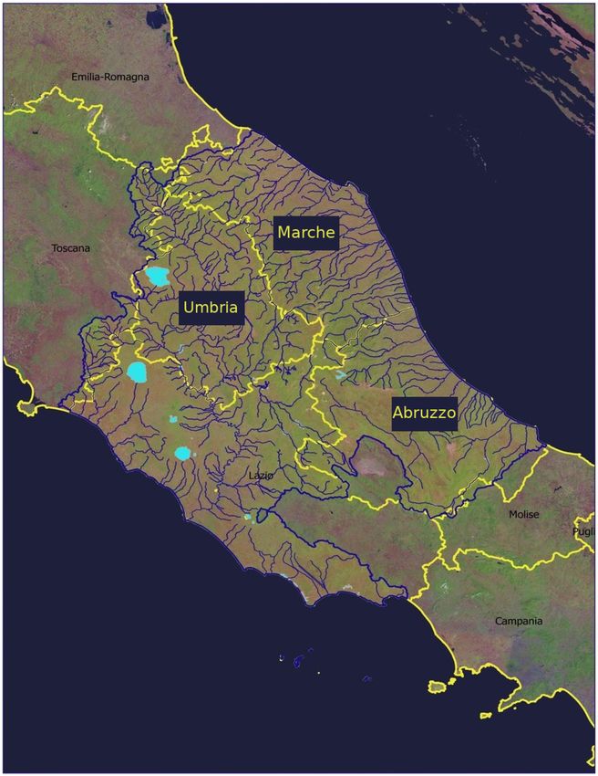
Figure 1. The Central Apennine Hydrological District (solid blue
to assess the possibility of defining a general-purpose alarm lines) and its main hydrography (thin blue lines). The north-eastern
index to highlight segments of drainage network where crit- boundary is delimited by the Potenza river basin, while the south-
ical stresses are expected. The idea of a hydrological-stress eastern limit is represented by the Sangro basin in Abruzzo. The
index arose from the collaboration with the Civil Protection; western side is delimited by the Tiber basin. Yellow lines indi-
this method is currently used in the framework of the agree- cate administrative boundaries of Italian regions. The three con-
ment between the Centre of Excellence CETEMPS and the sidered regions are highlighted: Umbria, Marche, Abruzzo (cour-
Abruzzo Regional Functional Center, where the former was tesy of the Tiber Basin Authority, https://www.autoritadistrettoac.
appointed as a competence centre of the Italian Civil Protec- it/i-numeri-del-distretto, last access: 10 June 2020).
tion and of the Abruzzo region as well. In detail, we devel-
oped and validated two hydrological-stress indices, related to
different flooding drivers over Central Italy. Due to its com- domain, devoid of climatological hydro-meteorological time
plex topography, the Central Apennine District (Central Italy, series. Before evaluating the performance of the hydrologi-
Fig. 1) is characterized by both large and structured catch- cal forecast through the use of these indices, a procedure for
ments (e.g. the Tiber and Aterno-Pescara; see next section) their validation on past floods is to be defined, by assimilat-
and short ephemeral tributaries and torrents, which have a ing observed meteorological data. The proposed evaluation
faster response to weather extremes and are more likely to be procedure is designed to tackle hydrological data scarceness
hit by a flash flood. Little information is available for those and takes advantage of signal theory processing methods.
small catchments, and hydrometric and/or discharge thresh- The paper is organized as follows: a detailed descrip-
olds are, hence, difficult to define. The discussed indices are tion of the chosen hydrological model and of the proposed
meant to be used in a complementary way, having the advan- hydrological-stress indices is reported in Sect. 2, while a de-
tage of being strongly user-oriented, as they are calibrated tailed description of the validation methods is provided in
taking into account a correspondence between the Civil Pro- Sect. 3. In Sect. 4 the geographical framework of the study
tection alarm level issued and index threshold. The innova- area is described, and in Sect. 5 the application of the pro-
tive nature of the presented hydrological-stress indices lies in posed approach to several case studies is discussed.
the definition of a unique index threshold, associated with an
alarm state, which assumes the same value over each point
of the drainage network reconstructed by the model. The in-
dices have been conceived to be applied over an interregional
https://doi.org/10.5194/hess-25-1969-2021 Hydrol. Earth Syst. Sci., 25, 1969–1992, 2021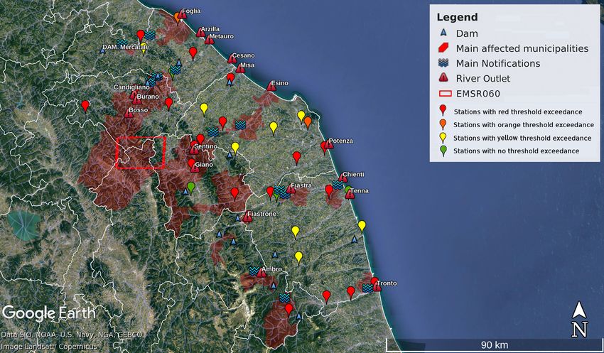
1972                                                 A. Lombardi et al.: Flood case studies in the Central Apennine District

2     Cetemps Hydrological Model                                   nuity equation is expressed through the following simplified
                                                                   form:
The Cetemps Hydrological Model (CHyM hereafter) has
                                                                   ∂Q ∂F
been developed at the Centre of Excellence CETEMPS, since             +    = q,                                                 (1)
2002 (Verdecchia et al., 2008b; Coppola et al., 2007). The         ∂x   ∂t
original purpose was the development of an operational hy-         where F is the flow cross-sectional area, Q is the flow rate
drological model for flood alert mapping (Tomassetti et al.,       of water discharge (m3 /s), q is the rate of lateral water inflow
2005). However, CHyM has also been applied in climatolog-          per unit of length, t is the time and x is the coordinate along
ical studies to investigate the effects of climate changes on      the river path.
the hydrological cycle (Coppola et al., 2014; Sangelantoni et         According to the shallow-water approximation, the Saint-
al., 2019).                                                        Venant equation for the momentum conservation is expressed
   CHyM is a fully distributed, physically based hydrological      through the rating curve approximation:
model, where the main hydrological processes are explicitly
simulated by a physically based numerical scheme.                  Q = αF m ,                                                   (2)
   An important characteristic of the model is the possibility
of simulating the hydrological cycle over any geographical         where α is the kinematic-wave parameter and m is the
domain with any spatial resolution up to the DEM resolution.       kinematic-wave exponent, adimensional, which is assumed
To this aim, the NASA SRTM (Shuttle Radar Topography               to be ≈ 1 for cylindrical river geometry. The kinematic-wave
Mission) DEM source file (https://lpdaac.usgs.gov/products/        parameter α has the dimension of a speed:
srtmgl3v003/, last access: 4 April 2020) is implemented in
the model with a native resolution of 90 m. Therefore, CHyM             S 1/2 R 2/3
                                                                   α=               ,                                           (3)
can simulate geographical domains with horizontal resolu-                  n (µ)
tions ≥ 90 m, even if the lower limit in choosing the spatial
                                                                   where S is the longitudinal bed slope of the flow element;
resolution deals with the validity of the numerical schemes
                                                                   n is Manning’s roughness coefficient, depending on the land
used to simulate the hydrological processes (e.g. the kine-
                                                                   use type µ; and R is the hydraulic radius, considered a linear
matic wave of shallow water, which is used to solve the con-
                                                                   function of the drained area D, according to the following
tinuity equation, is considered a good approximation with a
                                                                   formula.
horizontal resolution of a few hundred metres).
   For our national operational activity, we had divided the       R = β + γ Dδ ,                                               (4)
Italian territory into seven geographical sub-domains, each
one characterized by a spatial resolution which is chosen          where β, γ and δ are empirical constants to tune in the cali-
in order to optimize computational requirements (lower res-        bration phase. If the hydraulic radius is expressed in metres
olutions mean faster simulations) and the correct drainage         and the drained area is expressed in square kilometres, typ-
network extraction (higher resolutions mean more accurate          ical values of β, γ and δ are 0.0015, 0.35 and 0.33, respec-
drainage network reconstruction). In this paper, the opera-        tively.
tional spatial resolution associated with each sub-domain is          As for the surface flow outside the channel network, we
the same as that of the operational set-up (Taraglio et al.,       assume that the surface water depth y is constant over each
2019; Colaiuda et al., 2020). Starting from the NASA data,         grid point; therefore, the continuity equation assumes the fol-
the DEM is upscaled by applying the cellular automata spa-         lowing form:
tial interpolation technique (Coppola et al., 2007).
   In this section, the surface runoff calculation scheme is de-   ∂ϕ ∂y
                                                                      +    = ξ,                                                 (5)
scribed in detail; other parameterizations, such as evapotran-     ∂x   ∂t
spiration, infiltration, melting and return flow, are described
in Coppola et al. (2014).                                          where ϕ is flow rate over the longitudinal dimension (m2 /s)
                                                                   of the grid point and ξ is the rate of water inflow per unit of
2.1    Runoff                                                      area (m/s). The momentum equation has a linear relationship
                                                                   between the flow rate and the water depth, but Manning’s
To simulate the surface runoff, the continuity equation for        roughness coefficient is increased by a factor Mn as the wa-
surface routing and channel flow is explicitly solved. The         ter is assumed to flow with a lower speed. For the operational
flow direction for each grid point is established following the    simulations, the model default value of Mn for a river grid
minimum energy principle; therefore, the flow direction is         point is set to 4.5, but this parameter can be established dur-
assigned to the grid point located adjacently to the maximum       ing the calibration phase. An arbitrary drained-area threshold
downhill slope. The channel flow is computed according             of 100 km2 is set to distinguish the overland flow from the
to the kinematic-wave approximation of the shallow-water           channel flow, which is expected to occur for drained areas
equation (Lighthill and Whitham, 1955), where the conti-           wider than that threshold.

Hydrol. Earth Syst. Sci., 25, 1969–1992, 2021                                           https://doi.org/10.5194/hess-25-1969-2021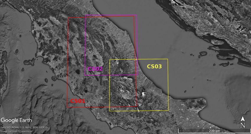
A. Lombardi et al.: Flood case studies in the Central Apennine District                                                       1973

2.2   CHyM flood stress indices for operational activities          case, fluvial and pluvial floods are combined and are suf-
                                                                    ficient from a few days to a few hours of intense rainfall,
The hydrological model, CHyM, has been widely calibrated            depending on the considered basin. For this reason, we de-
using climatological discharge time series of the river Po, as      veloped two different indices linked to the different flooding
reported in Coppola et al. (2014). To this aim, it is impor-        sources: the CHyM Alert Index (CAI), a pluvial flood in-
tant to note that the conditions of the Po are representative of    dex related to the limited capacity of a drainage systems, and
many alluvial rivers in Europe (Di Baldassarre et al., 2009).       Best Discharge-based Drainage (BDD), a fluvial flood index
   In general, long time series of flow discharge data are nec-     related to deluges from river channels. These indices and the
essary to calibrate and validate hydrological models. How-          associated stress thresholds are general; the signal of the hy-
ever, such data are not always available from all Italian re-       drological forecast is easy and quick to understand.
gions and, in many cases, rating curves used for the dis-              The hydrological-stress indices use the quantity of drained
charge estimation are not constantly updated. Furthermore,          water and the geomorphological characteristics of the differ-
hydrometric-level measurements are not available or less            ent basins. Although the units of measurement of the indices
available for major floods, when sensors installed along            are expressed in millimetres, they do not represent rainfall.
rivers stop working, due to severe meteorological conditions.       Both indices refer to the water accumulated on the ground
For this reason, many data in the upper part of the rating          over time. Three different thresholds for each of the two in-
curve are missed and larger errors in the discharge estima-         dices have been defined, in accordance with the protocols in
tion are often associated with higher-discharge bins. Finally,      use at the National Civil Protection Department. Since our
hydrometers are installed over main river channels and small        intention is to develop unique thresholds with the same val-
catchments are often excluded from discharge estimations,           ues at all grid points, we had to optimize threshold choice to
even if they are more prone to destructive flooding phenom-         maximize hit rate and minimize false alarms. In order to rea-
ena, especially in a complex-orography context. Hydrometric         sonably limit the scope of this paper, only results related to
and/or discharge thresholds are defined punctually and dif-         the moderate threshold (orange, pre-alert) are reported. The
fer for each sensor. In our stress index approach, discharge        reason for our preference for this threshold lies in the con-
and runoff are combined with geographical information re-           sideration of its meaning in the Civil Protection alert system.
lated to the upstream basin displacement, using other vari-         In fact, the orange threshold exceedance can be considered
ables, such as the hydraulic radius (a linear function of the       the most crucial one for the Civil Protection Department, be-
drained area) and time of concentration (that implicitly con-       cause its exceedance starts the activation of protection mea-
siders runoff conditions upstream). Therefore, stress indices       sures for people and infrastructure safety, as foreseen in risk
are able to give information in each point of the drainage          plans. The indices have been tested over a wide area in Cen-
network, and their mutual variation from upstream to down-          tral Italy, where many different catchments are located. Index
stream along the river path is proportional. For this reason,       validation is presented in “perfect conditions”, i.e. forcing
general thresholds, valid for all grid points of the drainage       the hydrological model with observed meteorological vari-
network, may be defined. Moving from discharge-only to              ables. In our operational activity, as stressed in Ferretti et
combined discharge-based and runoff-based indices, with the         al. (2020) and Colaiuda et al. (2020), CHyM uses observed
aim of calibrating such indices on a threshold basis for flood      meteorological data for the spin-up process and meteorolog-
alert purposes, gives us the possibility of calibrating and         ical model output to predict hydrological stress for the next
validating different information, which is not the discharge        24/48 h. Therefore, the index stress map is released from 6 to
amount but the river stress conditions, which is given by           48 h in advance in the operational set-up.
Civil Protection authorities using hydrometric thresholds, as
well as stress timing. Furthermore, the good estimation of          2.2.1   CHyM Alert Index
the stress state on a river channel is also provided by event re-
ports and from press releases in those locations where no sen-      The CHyM Alert Index (CAI) has long been used for the
sors are installed and, hence, no thresholds are defined. Since     operational activities of flood alert mapping in Central Italy.
the index validation is not numerical, the problem of missing       The CAI is calculated as a function of the rainfall drained
discharge data is overcome, the threshold-based calibration,        in each elementary cell of the simulated geographical do-
rather than physical quantities, being a sufficient condition       main. More specifically, the index is associated with each
for our purpose to validate an alert system.                        grid point, being the ratio between the total drained precipi-
   Moreover, it is important to highlight the influences of var-    tation and total drained area in the upstream basin, with re-
ious flooding drivers (Ashley et al., 2005; Balmforth et al.,       spect to the specific grid point. The proposed definition of the
2006) since pluvial flooding happens together with fluvial          hydrological-stress index also has a simple physical interpre-
flooding. Those flood scenarios were derived, for example,          tation: it represents the average precipitation drained in each
by adding rainstorms to the fluvial flood events, and this con-     cell, considering the rain falling over the whole upstream
dition is easily found when we consider Italian river basins        basin of the selected cell, during a time interval correspond-
with a size of up to even a few tens of kilometres. In this         ing to the mean time of concentration. A first version of the

https://doi.org/10.5194/hess-25-1969-2021                                        Hydrol. Earth Syst. Sci., 25, 1969–1992, 2021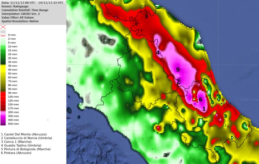
1974                                                 A. Lombardi et al.: Flood case studies in the Central Apennine District

CAI is described and tested in Tomassetti et al. (2005) and        where Q is the discharge predicted at time t and R is the hy-
Verdecchia et al. (2008a); in its initial formulation, the mean    draulic radius of the selected elementary cell, calculated as a
time of concentration of the upstream basin was considered         linear function of the upstream basin (see Eq. 4). BDD stress
a fixed term (36 or 48 h, depending on the basin dimension).       thresholds have been chosen following the same approach as
An updated version is presented in this work, where the av-        that used for the CAI thresholds, in order to match the three
erage time of concentration, tc , is explicitly calculated from    relevant hydrological criticality levels:
each drainage path k, down to the considered grid point of
coordinates i, j :                                                     1. ordinary stress – 3 mm/h,

           N t i,j
                                                                       2. moderate stress – 6 mm/h,
 i,j          k→ij
           X
tc     =              ,                                     (6)        3. high stress – 11 mm/h.
           k=1
                 N

where N indicates the total possible flowing paths.
                                                                   3    Materials and methods
   The time of concentration is computed for each grid point
of the geographical domain. It can be defined as the time re-      Floods are complex events, and data collection is not an
quired for a raindrop to travel from the hydraulically most        easy task to achieve in this matter. The Italian govern-
distant point in the watershed to the outlet. Each grid point is   ment introduced the Cadastre of Events, in response to
considered an outlet: namely, it may be a “mouth cell” drain-      Directive 2000/60/CE, a registry where relevant hydro-
ing toward a sea point, a “tributary mouth cell” draining to-      meteorological events are listed and associated with a het-
ward the interception with the main river or a cell draining       erogeneous database of different territorial data, organized
toward the border of the simulated domain. The water ve-           in geo-referred layers (e.g. flood time, localization and dam-
locity for each cell of the domain is computed according to        age). Data sources are not necessarily objective measure-
Eq. (3). The time of concentration used in the CAI calcu-          ments: collections may contain official Civil Protection re-
lation is an average calculated across all possible times of       ports and press releases, as well as other reports from local
concentration resulting from draining paths toward the con-        authorities. The official Hydrogeological Catastrophes GIS
sidered grid point.                                                (geographic information system) archive is available online
   The updated formula of the CAI is then the following:           at http://sici.irpi.cnr.it (last access: 9 June 2020). However,
        R Rt                                                       the database updating was concluded in 2000: after this date,
                   P (t, s) dtds                                   only a few Italian regions had moved to an alternative way
CAI = UP t−1t    R               ,                          (7)
                   UP ds                                           of data collection, mainly represented by regional databases
                                                                   with different data structures and classifications, freely or re-
where P is the precipitation available for the runoff. The in-     strictively accessible for external users. Considering the lack
tegral over the space s is calculated considering the whole        of official updated databases in the studied area, a huge but
upstream basin of the selected cell. For the stress state iden-    necessary effort was carried out to collect all available territo-
tification, three different thresholds have been defined, after    rial data for the selected case studies, following the approach
carrying out empirical tests: each threshold has been ade-         of the Cadastre of Events, in order to create our own database
quately chosen to qualitatively match the three different Civil    (ODB) with territorial, geo-referred information. Collected
Protection states of hydrological criticality, as defined by the   information in the ODB was used as reference data for the
head of the Civil Protection Department (2016):                    index validation process, discussed in the following section.
  1. ordinary stress – 30 mm/d,                                       The ODB was filled by searching for and classifying the
                                                                   following heterogeneous data about the considered flood
  2. moderate stress – 60 mm/d,                                    events:

  3. high stress – 110 mm/d.                                           – official Civil Protection event reports, issued by regional
                                                                         functional centres or environmental agencies;
The definition of each hydrogeological criticality level (and
related colour codes) is summarized in Table 1.                        – Copernicus Emergency Management Service;

2.2.2      Best Discharge-Based Drainage index                         – POLARIS database by CNR (National Research Coun-
                                                                         cil) IRPI (Research Institute for Geo-Hydrological Pro-
The BDD index is linked to the CHyM-predicted discharge                  tection);
and is calculated, for each grid cell of the drainage network,
according to the following formula:                                    – data from the AVI project;

                 Q (t)                                                 – press releases;
BDD(t) =               ,                                    (8)
                  R2

Hydrol. Earth Syst. Sci., 25, 1969–1992, 2021                                        https://doi.org/10.5194/hess-25-1969-2021
A. Lombardi et al.: Flood case studies in the Central Apennine District                                                                     1975

Table 1. Hydrogeological criticality levels officially defined by the Civil Protection authorities. Regional functional centres define hydromet-
ric thresholds, in relevant river sections. Those thresholds are based on the return period concept, in order to individuate the criticality level
to be assigned to the whole warning area (definitions conform to Deliberation no. 659/2017 of the Abruzzo Regional Council, Deliberation
no. 148/2018 of the Marche Regional Council and Deliberation no. 2312/2007 of the Umbria Regional Council).

  – photographic documentation from social media                           Italian region by local Civil Protection authorities (regional
    (e.g. YouTube, YouReporter), reporting major rainfall                  functional centres) at the station level (Fassi et al., 2008;
    events, floods and landslides causing direct human                     Brandolini et al., 2012; Mysiak et al., 2013). A colour code
    consequences and damage in the investigated period;                    is then assigned to each hydrometric threshold (see details
                                                                           in Table 1), indicating four different alarm levels, corre-
  – available hydrometric-level time series and thresholds,                sponding to specific hydraulic risk management actions, ac-
    where updated (from the Dewetra Platform, Italian Civil                tivated at an institutional level (Italian Legislative Decree
    Protection Department and CIMA Research Founda-                        No. 01/2018). However, as recognized by the Italian Insti-
    tion, 2014).                                                           tute for Environmental Protection and Research (ISPRA),
                                                                           the hydrometric level is a strongly non-stationary variable,
   The above-listed information was not all available for the
                                                                           as it is influenced by riverbed erosion and deposition pro-
same case study (CS); for this reason, a summary of the val-
                                                                           cesses (Braca et al., 2013). The hydrometric zero needs to
idation material found for each event is reported in Table 2.
                                                                           be recalibrated, establishing an updating frequency adequate
Moreover, to provide an overview of the data collection geo-
                                                                           for the river flow regime and local hydrogeological fac-
graphical distribution, the same information listed in Table 2
                                                                           tors. Moreover, the calibration should be carried out after
has been geo-referred and is shown in the maps of Figs. 2,
                                                                           flood occurrences, when the riverbed shape is significantly
3 and 4. Besides the territorial information, other hydrolog-
                                                                           modified. Then, the hydrometric thresholds need to be re-
ical data were used for the validation process. The Italian
                                                                           vised correspondingly. After the application of Italian Law
ministerial decree (DPCM), issued on 27 February 2004 and
                                                                           No. 183/1989, the management of the gauge’s network and
concerning the “Operating concepts for functional manage-
                                                                           data collection is devolved to the regional authorities. Even
ment of national and regional alert system during flooding
                                                                           though a territorial approach is useful for a rapid response
and landslide events for Civil Protection activities purposes”,
                                                                           to risk scenarios, competency fragmentation among different
establishes the regional functional centres to acquire and col-
                                                                           entities has caused inhomogeneities in hydro-meteorological
lect real-time data from monitoring networks. Hydrometric
                                                                           data availability and quality (e.g. rating curve updates, his-
levels are identified as the quantities to be monitored in or-
                                                                           torical hydro-meteorological data time series, hydrometric
der to assign the critical level for, at least, moderate and
                                                                           threshold availability for all stations) with significant differ-
high hydraulic risk to each warning area, through the def-
                                                                           ences among the 20 Italian regions.
inition of thresholds. Article 5 of the same decree defines
                                                                              For all the aforementioned reasons, a deterministic hydro-
that the real-time validation of prediction systems is made
                                                                           logical flood prediction validation over a wide, interregional
through the monitoring of moderate and high hydrometric-
                                                                           area can be challenging or not universally applicable, due
level threshold exceedances, for the main river channels. Sec-
                                                                           to missing or obsolete information. Moreover, the discharge
ondary drainage networks with drained areas of less than
                                                                           computation in hydrological models is affected by system-
400 km2 are not included in this kind of validation.
                                                                           atic biases when the hydrological network is exploited for
   The definition of water level critical thresholds (Italian
                                                                           hydropower production, irrigation, or industrial and domes-
Law No. 59/2004; Fassi et al., 2008) is carried out for each

https://doi.org/10.5194/hess-25-1969-2021                                                 Hydrol. Earth Syst. Sci., 25, 1969–1992, 2021
1976 A. Lombardi et al.: Flood case studies in the Central Apennine District
Table 2. Summary of relevant damage reported for each case study and information sources used.
Case study Date Region Reported damage Information sources
OR PR V
√ √ √
CS01 11–12 Nov 2013 Umbria Interruption of several roads and bridges, iso-
lated villages, damage to buildings and roads, a
hospital isolated
Important notes from OR
The large dams in the Tiber basin (Montedoglio
and Corbara on the Tiber and Casanuova on the
river Chiascio) played a crucial role in the stor-
age of upstream incoming volumes, allowing
the lamination and the misalignment of the full
floods downstream.
√ √ √
CS02 11–12 Nov 2013 Marche Interruption of several roads, houses evacuated,
isolated villages and two fatalities
Important notes from OR
The large dams in the Foglia, Metauro, Chienti
and Tronto basins played a crucial role in the
storage of upstream incoming volumes and al-
lowed the lamination and the misalignment of
the full floods downstream.
√ √
CS03 12–13 Nov 2013 Abruzzo Flooding phenomena affected the small X
Abruzzo rivers: interruption of several roads,
damage to buildings and roads.
OR: official Civil Protection report; PR: press releases; V: videos.
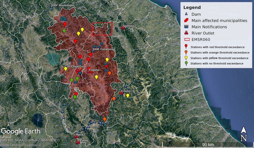
Figure 2. Geo-referred information of the ODB for CS01, Umbria region, with localization of main recorded floods (blue waves), hydrometric
stations used for the indices’ validation (pinpoints). Red triangles indicate the position of outlets of the main rivers involved, while blue
triangles indicate the presence of dams. Hydrometric station pinpoints are coloured according to the maximum hydrometric threshold reached
during the event. Municipality areas affected by flooding are filled in red. The red rectangle represents the involved area published on the
Copernicus Emergency Management Service platform (https://emergency.copernicus.eu/mapping/list-of-components/EMSR060, last access:
9 June 2020). © Google Earth.
Hydrol. Earth Syst. Sci., 25, 1969–1992, 2021 https://doi.org/10.5194/hess-25-1969-2021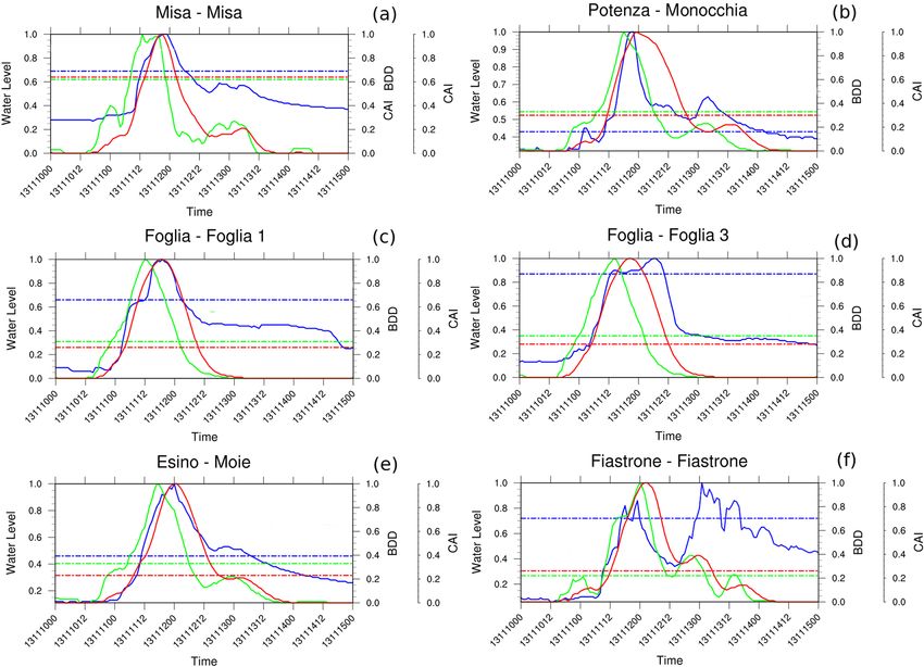
A. Lombardi et al.: Flood case studies in the Central Apennine District                                                                  1977

Figure 3. Geo-referred information of the ODB for CS02, Marche region, with localization of main recorded floods (blue waves), hydrometric
stations used for the indices’ validation (pinpoints). Red triangles indicate the position of outlets of the main rivers involved, while blue
triangles indicate the presence of dams. Hydrometric station pinpoints are coloured according to the maximum hydrometric threshold reached
during the event. Municipality areas affected by flooding are filled in red. © Google Earth.

Figure 4. Geo-referred information of the ODB for CS03, Abruzzo region, with localization of main recorded floods (blue waves), hydro-
metric stations used for the indices’ validation (pinpoints). Red triangles indicate the position of outlets of the main rivers involved, while
blue triangles indicate the presence of dams. Hydrometric station pinpoints are coloured according to the maximum hydrometric threshold
reached during the event. Municipality areas affected by flooding are filled in red. © Google Earth.

tic usage; in most cases, data about water uptake are scanty or           may be unavailable during a severe event or damaged by the
incomplete, as they are collected by a variety of public and              flood.
private actors and difficult to obtain. Another common is-                   The hydrological-stress index validation was first as-
sue for the spatial validation relates to threshold inference in          sessed through a qualitative approach, by selecting the
ungauged areas. Alfieri et al. (2017) highlighted that floods             strongest recorded signal of upcoming severe events from the
and flash floods usually occur in ungauged catchments; for                hydrometric-level time series and verifying the actual occur-
those situations, post-event survey reports represent the only            rence of floods in the areas where they were forecasted. To
source of information. Besides, even if present, gauge data               this aim, hydrological-stress index maps are compared with

https://doi.org/10.5194/hess-25-1969-2021                                               Hydrol. Earth Syst. Sci., 25, 1969–1992, 2021
1978                                                 A. Lombardi et al.: Flood case studies in the Central Apennine District

ODB geo-referred maps. In addition, an objective analysis          Table 3. Contingency table structure used for the validation analy-
is carried out by applying both statistical dichotomous and        sis.
continuous scores.
                                                                                                         Observed
3.1    Statistical dichotomous analysis                                                        Yes                  No

Primarily, the index grid map was spatially co-located with              Estimated   Yes     Hit (H )       False Alarm (FA)
the hydrometers’ position by choosing the nearest grid point                         No     Miss (Mi)     Correct Negative (CN)
to the station geographical coordinates after verifying the
correspondence between the grid point upstream drained area
calculated by CHyM, with the real value declared in the offi-                 FA
                                                                   FAR =           .                                              (11)
cial station registry (where available).                                    H + FA
   As for the time co-location, both water level and indices’      The calibration of the indices’ thresholds was chosen to max-
time series are hourly, and it might appear straightforward        imize the hit rate H , though at the cost of a higher average
to investigate the potential threshold exceedances by com-         false alarm rate: choosing a lower threshold increases detec-
paring the same time step. However, during a flood wave, it        tion skills of events with high uncertainty, according to Al-
is not infrequent to have water level data corrupted by mea-       fieri et al. (2017). All listed scores range from 0 to 1, where
surement errors during the flood wave transition (i.e. a solid     1 is the optimal value for A and the POD, while 0 indicates
surface stationing for a certain period under the hydrometric      the best possible score for the FAR.
sensor). For this reason, the time location is carried out by
associating a mobile interval of 3 h (the target time step ±1)     3.2    Catch rate
of observations to each index time step. The choice of this
confidence interval is arbitrary, although it is based on the      The catch rate (CR) was estimated for each index, to in-
authors’ experience. The contingency table was then built,         vestigate effectiveness in detecting or missing correct flood
for each station point and for each index, considering the         warnings. To this aim, the orange (moderate) hydrometric-
match between the co-located moderate hydrometric thresh-          level threshold exceedances (THR2s) were chosen as a term
old exceedances (THR 2 in Table 1) and the moderate index          of comparison with the corresponding moderate CAI and
threshold exceedances. Differently from water level thresh-        BDD index thresholds. A match occurs when the hydromet-
olds, CAI and BDD index thresholds have the same value             ric THR2 is exceeded and the moderate index threshold is
for all the grid points of the drainage network. These numer-      exceeded or when the hydrometric THR2 is not exceeded
ical thresholds are 6 mm/h for BDD and 60 mm/d for CAI,            and the moderate index threshold is not exceeded, within a
respectively; the choice of these values is justified a posteri-   24 h time range. A Boolean value 0/1 is then assigned when
ori considering the performances of the proposed indices for       a match occurs. CR is calculated as the ratio between the
different severe events analysed, during 10 years of opera-        number of correct matches found and the total number of
tional activity (Colaiuda et al., 2020). Under the most natural    analysed stations N:
conditions and with continuous updating of the hydrometric                XN 1
thresholds depending on the morphodynamic variability in           CR =       i=1 N
                                                                                    CESAi .                                 (12)
the basin, the proposed threshold levels for BDD and CAI
should appear very close to the water level threshold for the      Here the abbreviation CESA stands for correct estimated
specific site.                                                     state of alert for the i sensor, which assumes a value of 1
   The dichotomous scores include the accuracy (A), the            when estimation matches observation and a value of 0 when
probability of detection (POD), the false alarm ratio (FAR).       that match does not occur.
To build such a table, a flood event is considered an ob-
                                                                   3.3    Time peak analysis
served yes/no event if the water level exceeds/does not ex-
ceed the empirical threshold; a flood event is an estimated        In order to further evaluate the timing accuracy of the BDD
yes/no event if the estimated index exceeds/does not exceed        index and CAI, all the available observed water level time
the BDD and CAI thresholds (Table 3). The A, POD and FAR           series were compared to the indices’ time series. Because of
scores are defined as follows:                                     the comparison between two different physical quantities, the
           H + CN                                                  chosen statistical scores are typically used for signal studies.
A=                      ,                                   (9)    The first statistical analysis was made through the calculation
       H + Mi + FA + CN
                   H                                               of the lag time peak (LTP), to investigate the simultaneity
          POD =         ,                                  (10)    of occurrence between the water level peak and the indices
                 H + Mi
                                                                   peak. According to the Italian ministerial directive concern-
                                                                   ing “Operational guidelines for emergency management”, is-
                                                                   sued on 3 December 2008, a lag time of “a few hours” (less

Hydrol. Earth Syst. Sci., 25, 1969–1992, 2021                                        https://doi.org/10.5194/hess-25-1969-2021
A. Lombardi et al.: Flood case studies in the Central Apennine District 1979
than 12 h) is estimated to be between an event occurrence y(j ) of N and M components, respectively, an N-by-M ma-
and the activation of the Civil Protection coordination unit. In trix is built. An element V (i, j ) contains the Euclidean dis-
light of the above, we established that an adequate lag time tance between the ith element of the first sequence and j th
peak for flood prediction should not exceed 3 h. According element of the second sequence. For this matrix, a warping
to other authors (see, as an example, Rabuffetti et al., 2008), path W is defined as a contiguous set of L matrix elements,
the relative lag time peak (RLTP), defined as the ratio be- and the measure of misalignment d for the path W is given
tween the LTP and the average time of concentration of the by
upstream basin, can be calculated. P
i,j V (i, j )
3.4 Correlation time delay (CTD) d (W ) = 1 , (16)
2 L (L − 1)
The cross correlation (CC) is typically used in signal theory where the sum in the numerator is carried out over all the el-
(Rabiner and Gold, 1975; Rabiner and Schafer, 1978; Ben- ements belonging to the warping path W . The denominator
esty et al., 2004), for the assessment of similarity between is used to normalize different length sequences. The DTW
two signals. Given two discrete series x(t) and y(t), each index is then calculated as the minimum value of d(W ), con-
one of N components, the cross correlation is calculated as sidering all the possible paths W .
the dot product of the series:
XN DTW = d (W ) (17)
CC = i=1
x (ti ) y (ti ) . (13)
For instance, if the two considered sequences are aligned and
The same product can be calculated, shifting the two signals have the same number of components (N = M), the optimal
of a time lag L: path will be the N diagonal elements of matrix V.
XN The DDTW (Fig. 5) algorithm implementation replaces
CC (L) = x (ti ) y (ti + L) . (14) the data time series with their first derivative and the Eu-
i=1
clidean distance is measured on them. The first derivative has
The correlation time delay (CTD) is then defined as the value been calculated for each time series as follows:
of time lag L that maximizes the previous product.
(x [i] − x [i − 1]) + ((x [i + 1] − x [i − 1])/2
D (x[i]) = . (18)
CTD = CC (L) (15) 2
CTD represents an estimation of time shift between two se-
ries; therefore, we found this score to be suitable to mea-
sure the effectiveness of the signal given by the hydrological- 4 Study area description
stress indices.
The study area covers the Central Apennine District (Fig. 1),
3.5 Derivate dynamic time-warping analysis with an extension of 42 506 km2 and about 8 million inhab-
itants. The northern part, which includes the upstream basin
Dynamic time warping (DTW; Berndt and Clifford, 1994; of the Tiber from the confluence with the river Nera, is char-
Keogh and Ratanamahatana, 2005; Maier-Gerber et al., acterized by a less dense draining network with respect to
2019; Di Muzio et al., 2019) allows us to stress (or com- the lower part of the basin. This area has complex hydrogra-
press) two time series to achieve a reasonable fit between phy, characterized by both perennial rivers, constantly fed by
them. The idea of the method is that the similarity between groundwater, and seasonal streams, which are activated only
two sequences can be estimated by “warping” the time axis in rainy periods. Moreover, plenty of artificial reservoirs and
of one (or both) sequences, to achieve a better alignment. Al- hilly ponds take up surface runoff water. The Adriatic slope
though DTW has been successfully used in many domains, is located over the central part of the district, extending from
it may lead to obtaining incorrect results; as an example, the the upper Marche region (the river Potenza) to the southern
technique may fail in finding the optimal alignment because part of the Abruzzo region (river Sangro). The lower path of
a feature (i.e. peak or local minimum) in one sequence is the Tiber is also part of this area, together with the tributaries
higher or lower than its corresponding feature in the other on the left bank, from the Nera to Aniene rivers.
sequence. This area is affected by inundations along major rivers,
To overcome this problem, Keogh and Pazzani (2001) pro- as well as flash floods in torrents and minor streams, espe-
posed the computation of warping using the local derivative cially on the heels of the ridge, where high-intensity rain-
of the time series to be compared and called this algorithm storms cause lowland flooding. Most of the drainage net-
Derivative Dynamic Time Warping (DDTW). work is characterized by significant water storage (with a
The numerical procedure for the DTW calculation can be quite constant spring flow rate during the year) and marked
summarized as follows: given two discrete series x(i) and by hydroelectric power plants, built since the last century
https://doi.org/10.5194/hess-25-1969-2021 Hydrol. Earth Syst. Sci., 25, 1969–1992, 20211980 A. Lombardi et al.: Flood case studies in the Central Apennine District
Figure 5. Graphical representation of DDTW correspondences between two first derivatives of time series x(t) and y(t). In this case, time
series are represented by two generic profiles of the hydrometric water level and the BDD index, at the same station point (from Keogh and
Pazzani, 2001).
(Tiber Basin Authority, 2010). The peak discharge variation
depends on the storage type: generally, the effect of a reser-
voir on flood control results from a combination of regulated
and unregulated storage (Volpi et al., 2018). The former, used
in the analysed area, is less efficient in flood-peak reduction
than regulated storage, as it begins filling even before it is
needed. Moreover, the effect of a flood control reservoir de-
pends on the combination of off-stream or on-stream deten-
tion ponds as reported by Ravazzani et al. (2014). Dams and
reservoirs play an important role during flood events (Rodda,
2011; Kundzewicz et al., 2014; Ayalew et al., 2017; Habets et
al., 2018): this role is not always favourable; they adversely
Figure 6. Three CHyM geographical domains used for the simula-
affect the extent of an inundation due to dike breaches, block- tion of the corresponding CSs. The red square encloses the Umbria
age of bridges and culverts by debris. Anyway, weak co- region and the rest of Tiber basin for CS01; the pink square refers
ordination between different actors involved in water re- to CS02 (Marche region), and the yellow square encompasses the
source management may significantly affect flood dynamics. Abruzzo region for CS03. © Google Earth.
In multi-purpose reservoirs, competing interests represent a
key issue in flood regulation: irrigation, hydropower gener-
ation and flood control generally compete, even when the information are provided. Details of links pointing to each
reservoir is owned by a single country or agency. This con- source used to organize the ODB are provided in the Supple-
flict of interests is heightened when the basin is interregional, ment, where all hit municipalities and affected rivers are also
as in the case of the Central Apennine District. For those rea- listed.
sons, the WMO (2009) recommends carefully evaluating the
flood timing and dynamics. 5.1 Synoptic analysis
On 11 November 2013, a large synoptic-scale meteorological
system originated from the Atlantic Ocean and moved into
5 Results and discussion
the Mediterranean area. In particular, the cold air coming in
from southern France has induced rapid cyclogenesis on the
In this section, the analysis of a meteo-hydrological event
Gulf of Genoa. The barometric minimum moved southward
that occurred in Central Italy on 11–13 November 2013 is
along the Italian Peninsula and reached the Tyrrhenian Sea
proposed. The 3 d event was characterized by intense precip-
on 12 November. The persistence of the occluded front over
itation, involving the whole Central Apennine ridge and three
Italy caused heavy and long precipitation, initially affecting
different regions, progressively affecting the Adriatic side of
northern regions and, progressively, central and southern ar-
the central part of Italy, moving from north to south. To better
eas, as the minimum moved toward the Libyan coast, on 13
organize our analysis, the event was divided into three differ-
November. The precipitation was widespread, with a huge
ent case studies, related to three different regions involved:
amount. According to the event reports from regional Civil
Umbria (CS01), Marche (CS02) and Abruzzo (CS03). The
Protection authorities, registered precipitation amounts were
CHyM simulations were set to three different geographical
almost 300 mm/72 h in several areas, mainly located along
domains, as shown in Fig. 6. The event was very intense and
the Apennine ridge, between the Marche and Umbria regions
caused much damage and a few fatalities in all regions; an
(Fig. 7).
overview of the phenomenon is reported in Table 2, where
relevant information about observed effects and sources of
Hydrol. Earth Syst. Sci., 25, 1969–1992, 2021 https://doi.org/10.5194/hess-25-1969-2021A. Lombardi et al.: Flood case studies in the Central Apennine District 1981
Figure 7. Total accumulated rainfall (spatialization from rain gauge official network) during the event, from 11 November 2012 00:00 UTC
to 13 November 2013 23:00 UTC (picture generated from the Dewetra Platform, Italian Civil Protection Department and CIMA Research
Foundation, 2014). The localization of the six rain gauges are indicated on the map: (1) Castel del Monte station (Abruzzo region), (2)
Castelluccio di Norcia station (Umbria region), (3) Conca 1 station (Marche region), (4) Gualdo Tadino station (Umbria region), (5) Pintura
di Bolognola station (Marche region), (6) Pretara station (Abruzzo region). The rain gauges recorded significant accumulated rain (up to
400 mm/72 h, purple area).
5.2 Case study analysis lines; white lines indicate alert zone boundaries, defined
by the Civil Protection, reddish areas encompass the ad-
ministrative boundaries of the main affected municipali-
Hydrological simulations were carried out over a geograph-
ties (i.e. where a flood was reported), while the small blue
ical domain larger than the areas where floods were actu-
triangles highlight the main water reservoirs located in-
ally observed, in order to verify the absence of predicted
side the domain. In Figs. 2 and 3, red rectangles repre-
hydrological-stress conditions in those areas where the hy-
sent the flood-affected area published on Copernicus Emer-
drological criticality level has not been exceeded. Hydrolog-
gency Management Service platform (EMS Rapid Map-
ical simulation was set by using a spin-up time of 120 h for all
ping activations (EMSR060), https://emergency.copernicus.
case studies, before the day of the hydrological event. Given
eu/mapping/list-of-components/EMSR060, last access: 9
the small extension of the involved catchments, 120 h of spin-
June 2020).
up seems to be enough for the model initialization. It should
be noticed that stress indices are used to detect hydrologi-
cal situations where relevant discharges, driven by significant 5.2.1 Case study 1 – Umbria region
rainfall events in a short time (a few hours to a few days) are
present. The selected case studies affected different regions From 11 to 12 November 2013, a severe weather event hit
of Central Italy characterized by catchments of different sizes the Umbria region. The event was mainly concentrated over
and geomorphological characteristics, allowing the evalua- the north-eastern part of the region, along the administrative
tion of index feasibility in heterogeneous domains. Spatial boundary with the Marche region. According to the data pro-
and temporal characteristics of the hydrological simulations vided by the official hydro-meteorological monitoring net-
are reported in Table 4. work, precipitation was persistent and intense, resulting in
As discussed in Sect. 3, the ODB information about exceptional amounts, up to 440 mm in the Castelluccio di
case studies was geo-referenced on a Google Earth maps Norcia station and 330 mm in Gualdo Tadino in 72 h (see
(Figs. 2, 3, 4). The blue wave symbols indicate reported Fig. 7). Flooding affected main rivers, as well as small catch-
inundations, and the pinpoints show the hydrometers dis- ments (river outlet highlighted in Fig. 2), such as the Tiber,
placement; the colour assigned to each pinpoint highlights the upper Chiascio, and the Topino basins. In particular, the
the observed state of alert, namely, the hydrometric thresh- flooding on the river Sentino, flowing along the boundary
old exceedances (see Table 1 for further details). On the with the Marche region, caused damage to 12 residential
same maps, the drainage network is represented by blue buildings and temporarily isolated the Branca hospital, due
https://doi.org/10.5194/hess-25-1969-2021 Hydrol. Earth Syst. Sci., 25, 1969–1992, 2021You can also read