The all-sky PLATO input catalogue - Astronomy & Astrophysics
←
→
Page content transcription
If your browser does not render page correctly, please read the page content below
A&A 653, A98 (2021)
https://doi.org/10.1051/0004-6361/202140717                                                                           Astronomy
c ESO 2021                                                                                                             &
                                                                                                                      Astrophysics

                                  The all-sky PLATO input catalogue?
   M. Montalto1,2 , G. Piotto1,2 , P. M. Marrese3,4 , V. Nascimbeni1,2 , L. Prisinzano5 , V. Granata1,2 , S. Marinoni3,4 ,
S. Desidera2 , S. Ortolani1,2 , C. Aerts14,15,16 , E. Alei6 , G. Altavilla3,4 , S. Benatti5 , A. Börner7 , J. Cabrera8 , R. Claudi2 ,
      M. Deleuil12 , M. Fabrizio3,4 , L. Gizon17,18,19 , M. J. Goupil9 , A. M. Heras10 , D. Magrin2 , L. Malavolta1,2 ,
    J. M. Mas-Hesse13 , I. Pagano11 , C. Paproth7 , M. Pertenais7 , D. Pollacco20,21 , R. Ragazzoni1,2 , G. Ramsay24 ,
                                                   H. Rauer8,22 , and S. Udry23
                                                  (Affiliations can be found after the references)

                                                 Received 3 March 2021 / Accepted 16 May 2021

                                                                   ABSTRACT

Context. The ESA PLAnetary Transits and Oscillations of stars (PLATO) mission will search for terrestrial planets in the habitable zone of solar-
type stars. Because of telemetry limitations, PLATO targets need to be pre-selected.
Aims. In this paper, we present an all sky catalogue that will be fundamental to selecting the best PLATO fields and the most promising target stars,
deriving their basic parameters, analysing the instrumental performances, and then planing and optimising follow-up observations. This catalogue
also represents a valuable resource for the general definition of stellar samples optimised for the search of transiting planets.
Methods. We used Gaia Data Release 2 astrometry and photometry and 3D maps of the local interstellar medium to isolate FGK (V ≤ 13) and M
(V ≤ 16) dwarfs and subgiant stars.
Results. We present the first public release of the all-sky PLATO input catalogue (asPIC1.1) containing a total of 2 675 539 stars including
2 378 177 FGK dwarfs and subgiants and 297 362 M dwarfs. The median distance in our sample is 428 pc for FGK stars and 146 pc for M dwarfs,
respectively. We derived the reddening of our targets and developed an algorithm to estimate stellar fundamental parameters (T eff , radius, mass)
from astrometric and photometric measurements.
Conclusions. We show that the overall (internal+external) uncertainties on the stellar parameter determined in the present study are ∼230 K (4%)
for the effective temperatures, ∼0.1 R (9%) for the stellar radii, and ∼0.1 M (11%) for the stellar mass. We release a special target list containing
all known planet hosts cross-matched with our catalogue.
Key words. catalogs – astrometry – techniques: photometric – planets and satellites: terrestrial planets – stars: fundamental parameters –
ISM: structure

1. Introduction                                                             including all the ancillary devices like baffling, electronics, etc.)
The PLATO mission (Rauer et al. 2014, 2016) is the third                    made up with refractive 20 cm-class optical elements with a very
medium-class mission in the ESA Cosmic Vision programme.                    wide field (about 40 degrees in diameter) and a 12cm diameter
Its ambitious goals are the detection and characterisation of               equivalent aperture.
terrestrial planets around solar-type stars as well as the study                 Each camera field of view is almost covered by an array
of the properties of host stars. The focus of PLATO is on                   of detectors totaling 1037 square degrees, and 24 cameras are
long-orbital-period terrestrial planets that are also in the hab-           arranged in four groups of six cameras each, co-aligned to four
itable zone of solar-type stars. PLATO is designed for the                  slightly overlapping fields of view. The S/N of each star will
discovery of Earth-analogue planets under potentially favourable            therefore be dependent on its precise location within the overall
conditions for the development of life.                                     PLATO field of view. The combined field of view of the sys-
    PLATO will achieve its goals by detecting the low-amplitude             tem of cameras amounts to a total of about 2100 square degrees
dips in stellar brightness produced by planets transiting in front          (Ragazzoni et al. 2015; Magrin et al. 2018). The remaining two
of the disk of their parent stars. The mission is designed and opti-        cameras are optimised for fast monitoring of very bright stars,
mised to continuously monitor two Long-duration Observation                 their colour measurements (e.g., Grenfell et al. 2020), and fine
Phase (LOP) fields, each one for up to three years, and has the             guidance and navigation. Their focal plane is equipped with
capability to monitor some additional fields during shorter times,          frame transfer detectors that allow for a coverage somewhat
up to three months each (‘Step and stare’ Observation Phase,                larger than 600 degrees. The geometry of the covered patches
SOP). The precise observing strategy will be decided at a later             in the sky is kept symmetric, under nominal conditions, for 90
stage (two years before launch at the latest), taking advantage of          degree rotations around the line of sight to keep the same cov-
the advances in the field at that time.                                     erage of the field of view throughout a pointing and to allow
    PLATO will employ an array of 26 cameras (hereafter ‘cam-               continuous in-flight calibration among different cameras. Com-
eras’ signifies the telescope optics and the focal plane assembly,          pliance with the performance specifications is computed using
  ?
    The catalogue described in this article is only available at MAST as
                                                                            models for the degradation of the performances over the mission
a High Level Science Product via https://dx.doi.org/10.17909/               lifetime, mainly due to a moderate degradation of the through-
t9-8msm-xh08 and https://archive.stsci.edu/hlsp/aspic, in                   put, due to the choice of rad-hardened glasses for the optical
the SSDC tools page (https://tools.ssdc.asi.it/asPICtool/)                  elements most exposed to cosmic radiation (Magrin et al. 2016;
and at the CDS via anonymous ftp to cdsarc.u-strasbg.fr                     Corso et al. 2018), and to the worst scenario in which the detec-
(130.79.128.5) or via http://cdsarc.u-strasbg.fr/cgi-bin/                   tors or electrical systems of two of the cameras could fail by the
viz-bin/cat/J/A+A/653/A98                                                   End Of Life (EOF).

                                                        Article published by EDP Sciences                                         A98, page 1 of 23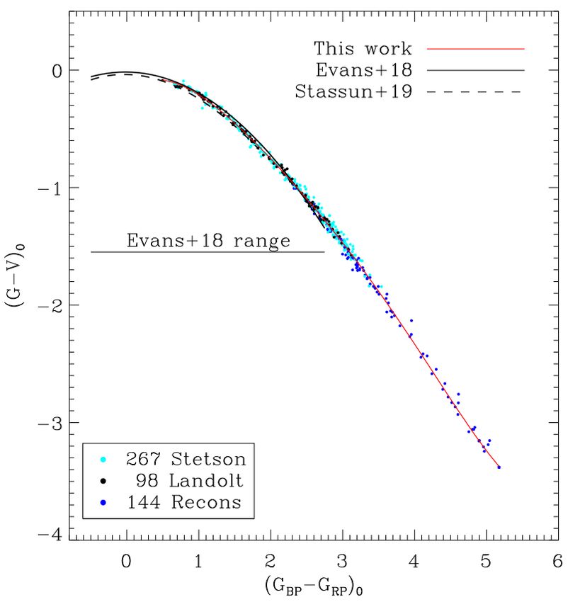
A&A 653, A98 (2021)

Because of limits on the telemetry rate from the satellite to                Previous attempts to produce this catalogue showed that this
Earth, it is not possible to download full CCD images at a suf-          is not a trivial task. In particular, it is hard to robustly dis-
ficient rate to detect planets; therefore, it is necessary to pre-       criminate between dwarfs and evolved stars without accurate
select PLATO targets. For a subsample of targets, customised             knowledge of the absolute luminosities of sources. Reduced
‘postage stamps’ (imagettes) are downloaded to ground; for the           proper motions were employed in the past to this purpose
remaining selected stars, centring and photometry will be per-           (Nascimbeni et al. 2016), but this technique is now superseded
formed on board and then downloaded to ground. Other, pre-               by the availability of trigonometric parallaxes from Gaia Data
vious space missions followed the same approach. The CoRoT               Release 2 (DR2) (Gaia Collaboration 2016, 2018)1 , essentially
Exo-Dat catalogue (Deleuil et al. 2009), the Kepler input cata-          for all targets of PLATO interest, permitting accurate determina-
logue (KIC; Brown et al. 2011), the K2 Ecliptic Plane Input Cat-         tion of distances and therefore of absolute luminosities.
alogue (EPIC; Huber et al. 2016), and the TESS input catalogue           After ESA adoption (in June 2017), PLATO recently entered
(TIC; Stassun et al. 2018, 2019) were produced to select the best        the full industrial development phases C-D (March 2020) to be
targets for exoplanet searches.                                          ready for launch in 2026. At this development stage, the selec-
     In this paper, we present the all-sky PLATO input catalogue         tion of the PLATO LOP fields is not yet finalised (it will be two
(asPIC), whose main purpose is to serve as the primary database          years before launch). The present work is focused on the asPIC.
for the selection of PLATO targets. Establishing the properties          This catalogue is made publicly available to the community and
of PLATO host stars is crucial to determining the properties of          it will be updated whenever relevant changes occur, including
transiting planets; for example, the uncertainty on their radii is       new Gaia releases.
directly related to the uncertainty on the host-star radius. The         After briefly describing the mission requirements defining
classical properties of planet hosts are also essential to mod-          PLATO stellar samples in Sect. 2, we describe the target selec-
elling the stars using asteroseismology. Also, the habitability of       tion criteria in Sect. 3. Then, in Sect 4, we describe how we
a given planet depends on the properties of the host star, among         account for reddening and absorption in our analysis. Our stel-
other factors. Moreover, knowing the values of stellar parame-           lar parameter pipeline is presented in Sect. 5. In Sect. 6, we
ters permits the statistical study of the frequency of planets as a      compare our results with those published in various literature
function of stellar type, metallicity, environment, and so on (e.g.,     sources. In Sect. 7, we describe a special list of known planet
Howard et al. 2012; Bryson et al. 2020).                                 host stars included in the catalogue release. Section 8 provides a
The construction of such a catalogue not only requires the iden-         brief summary of the present work.
tification, across the entire sky, of stars with the required spectral
type and luminosity class, but also requires that noise constraints
be accounted for to facilitate the detection of transiting plan-         2. PLATO stellar sample requirements
ets around the selected sources. Hence limits on the magnitude
range of the stellar samples are set according to mission require-       The four main PLATO stellar samples (named P1, P2, P4, and
ments and the degree of contamination of each target from neigh-         P5)2 will be observed in the wavelength range between 500 nm
bouring sources must be evaluated. The PLATO pixel scale will            and 1000 nm, and an additional colour sample will be observed
be 15 arcsec pix−1 on axis, which lies between that of Kepler (4         in two broad blue and red spectral bands spanning the 500–675
arcsec pix−1 ; Borucki et al. 2010) and that of TESS (21 arcsec          and 675–1000 nm wavelength ranges, respectively (Corso et al.
pix−1 ; Ricker et al. 2014).                                             2018). The science requirements for the PLATO stellar samples
     The optical quality of the PSF, although slightly variable          are listed below and summarised in Table 1 according to the
over the field of view and depending on the thermal status of            ESA Science Requirements Document (SciRD, PTO-EST-SCI-
the cameras, is expected to encompass an area of a few pixels            RS-0150_SciRD_7_0). The definition of the PLATO samples
(see also Gullieuszik et al. 2016; Umbriaco et al. 2018). Conse-         requires knowledge of the visual apparent magnitude V because
quently, it is expected that several sources, especially in crowded      the SciRD adopts this magnitude as reference to identify suf-
fields, will be blended into a single brightness measurement area        ficiently bright targets for ground-based spectroscopic follow-
and they may become the cause of false positive signals (e.g.,           up. The V magnitude we used to select the targets comes from
Santerne et al. 2015; Fressin et al. 2013). More specifically, the       our own calibrated transformation of Gaia DR2 magnitudes and
asPIC will be used to:                                                   colours to the Johnson V band (Eq. (1)). This choice ensures the
     1. Select the optimal PLATO observing fields;                       maximum homogeneity of the V band photometry. The calibra-
     2. Select all FGKM dwarf and subgiant stars satisfying the          tion procedure is described in Appendix A. The colour transfor-
magnitude and signal-to-noise constraints defined in the PLATO           mation relation is
stellar sample requirements;
     3. Estimate basic stellar parameters for all targets, such as       (G − V)0 = c0 + c1 (GBP − GRP )0 + c2 (GBP − GRP )20
temperatures, radii, and masses;                                                     + c3 (GBP − GRP )30 + c4 (GBP − GRP )40 +
     4. Identify known variable stars, binaries, members of multi-
                                                                                     + c5 (GBP − GRP )50 ,                                 (1)
ple systems, active stars with bitmasks, and summarize the infor-
mation available from existing catalogues, that is, mainly Gaia
                                                                         where G, GBP , GRP are the Gaia DR2 magnitudes and the
and TESS releases;
                                                                         null subscript indicates colours dereddenend with the procedure
     5. Supply a list of all target contaminants up to a specific
                                                                         described in Sect. 4. The best-fit coefficients of the transforma-
angular distance from the target and up to a limiting magnitude,
                                                                         tion relation are reported in Table 2.
for the targets in the fields to be observed, in order to under-
stand their impact on photometric performances and because of            1
                                                                             Although Gaia EDR3 has now been released (Gaia Collaboration
the challenge that background contaminants pose to planetary             2021) this work is based on Gaia DR2. Future updates of the asPIC will
candidate validation;                                                    be based on Gaia DR3.
     6. Guide the organisation and optimisation of ground-based          2
                                                                            For historical reasons, the sample P3 has been eliminated, but the
follow-up strategies.                                                    numbering of the PLATO samples was left unchanged.

A98, page 2 of 23
M. Montalto et al.: The all sky PLATO input catalog
Table 1. Summary of science requirements for the PLATO stellar samples.
P1 P2 P4 P5 Colour sample
Stars ≥15 000 (goal 20 000) ≥1000 ≥5000 ≥245 000 300
Spectral type Dwarf and Dwarf and M Dwarfs Dwarf and Anywhere in
subgiants F5-K7 subgiants F5-K7 subgiants F5-late K the HR diagram
Limit V 11 8.5 16 13 –
Random noise (ppm in 1 h)A&A 653, A98 (2021)
Fig. 1. Absolute magnitude vs. reddening-free colour obtained from TRILEGALv1.6 simulations. Crosses represent simulated stars from a total
area of 100 square degrees in the NPF and the SPF, satisfying the conditions described by the labels at the top of each plot. The left and right
panels also show the analytical selection (red lines) described in Sect. 3.3 for FGK dwarfs and subgiants (FGK sample) and for M dwarfs (M
sample), respectively. In the diagram on the right, the blue dashed line represents a 10 Myr solar metallicity isochrone from the Padova database
(Bressan et al. 2012).
and empirical distributions of stars in the CMD, we proceeded passbands of Maíz Apellániz & Weiler (2018) and determined
by defining an analytical selection region, and estimated its the apparent visual magnitude V using the relation reported in
degree of completeness and contamination (Sect. 3.3). Finally, Appendix A. We corrected the apparent magnitudes of each sim-
in Sect. 3.5 we show that our selection does not imply any bias ulated star for extinction using the V band extinction tabulated
in the metallicity distribution of the selected stars with respect in the simulations and the relations given in Sect. 5.2 in order
to a sample of local stars (Sect. 3.4) and present the asPIC1.1 to convert the extinction in the V band to the extinction in the
catalogue resulting from our selection. Gaia bands. Figure 1 shows the intrinsic colour (reddening free)
As summarised in Sect. 2, the PLATO samples considered and absolute magnitude obtained from TRILEGALv1.6 simula-
here include an FGK dwarf and subgiant sample (limited to F5), tions. The left panel shows stars with V < 13, log g > 3.5 and
and an M dwarf sample. Considering the definitions reported 3870 K < T eff < 6510 K corresponding to our adopted limits for
in Table 5 of Pecaut & Mamajek (2013), spectral type F5 cor- the FGK sample, while the right panel shows stars with V < 16,
responds to T eff = 6510 K, or to an unreddened Gaia colour log g > 3.5 and T eff ≤ 3870 K (M sample). Figures 2 and 3 show
(GBP −GRP )0 = 0.587, and spectral type M0 corresponds to T eff = the distributions of effective temperatures (left panel) radii (mid-
3870 K or unreddened (GBP − GRP )0 = 1.84, where GBP and GRP dle) and masses (right) of the simulated stars. Magnitude limited
are the blue and red Gaia magnitudes, respectively. In addition, samples, like the ones we are considering, are dominated by hot-
dwarfs and subgiants have log g > 3.5. dwarfs and subgiants, because these stars are intrinsically more
luminous and therefore observable in a large volume.
We also repeated the simulations for fields located in the
3.1. Theoretical models
Galactic plane or at the Galactic poles. The intrinsic colours and
To determine and calibrate our selection criteria in an obser- magnitudes of the selected stars are perfectly compatible with
vational CMD, we used Galactic simulations from TRILE- the ones shown in Fig. 1. Larger uncertainties in the reddening
GALv1.6, (Girardi et al. 2005)3 . TRILEGAL is a population estimates occur for the Galactic plane and would lead to higher
synthesis code for simulating the stellar photometry of any levels of contamination, particularly for hot dwarfs and subgiants
Galaxy field. It allows the user to simulate the photometry in sev- (see also Sect. 3.3).
eral different broad-band photometric systems. Each simulation
we performed corresponds to an area of ten square degrees. The 3.2. Empirical control samples
simulations were centred at (l,b) = (65◦ , 30◦ ) and (l,b) = (253◦ ,
−30◦ ), and on four surrounding locations ten degrees apart from For FGK dwarfs and subgiants, as an empirical control sam-
the central fields in Galactic longitude or latitude. The two ple, we used stars from the RAVE DR5 survey (Kunder et al.
central fields correspond to the two provisional PLATO long- 2017). RAVE provides two sets of stellar parameters: those that
duration fields in the Northern and Southern Galactic hemi- are direct outputs of the stellar parameter pipeline and the cal-
spheres, that is the North PLATO field and the South PLATO ibrated parameters. Because the direct outputs are based on a
field (NPF and SPF, respectively). We considered the Gaia DR2 grid of synthetic spectra which may not match real spectra over
the entire domain of the parameter space, a calibration based
3
http://stev.oapd.inaf.it/cgi-bin/trilegal on reference stars is performed in order to minimise systematic
A98, page 4 of 23M. Montalto et al.: The all sky PLATO input catalog
Fig. 2. Distribution of effective temperatures (left panel), stellar radii (middle), and masses (right) for FGK sample stars from TRILEGAL
simulations.
Fig. 3. Distribution of effective temperatures (left panel), stellar radii (middle), and masses (right) for M sample stars from TRILEGAL simulations.
offsets. For example, surface gravities are calibrated using both the Mann et al. (2015) catalogue. Among other information, the
the asteroseismic log g values of 72 giants from Valentini et al. RECONS catalogue reports the apparent visual Johnson mag-
(2016) and the Gaia benchmark dwarfs and giants (Heiter et al. nitude of the targeted stars. Whenever multiple measurements
2015). We then adopted the calibrated parameters. We consid- for the same object were present in the catalogue, we averaged
ered stars with RAVE parameter ALGOCONV = 0 and S /N > their visual magnitudes. From the initial list of 348 entries we
50 to ensure the good quality of extracted parameters. A total obtained a list of 289 measurements for the individual objects.
of 122 167 stars were used. We analysed the distribution of The catalogue was cross-matched with Gaia DR2 and we then
RAVE stars in the absolute colour magnitude diagram con- selected stars with V < 16 that satisfy Eqs. (1) and (2) of
structed using Bailer-Jones et al. (2018) distances. We corrected Arenou et al. (2018) Gaia astrometric and photometric quality
the apparent magnitudes for extinction using the procedure pre- criteria and are classified as M-dwarfs6 , restricting the list to 195
sented in Sect. 44 . To identify the selection regions of dwarfs and stars. We then calculated the reddening as described in Sect. 4.
subgiants in the (GBP − GBP )0 , MG,0 plane, we considered a grid The right panel of Fig. 4 shows the absolute colour–magnitude
of 0.05 mag × 0.5 mag bins in colour and magnitude across the diagram corrected for reddening of the selected stars (open black
plane. We considered stars with V < 13, where the V band mag- circles) of this sample.
nitude was calculated with the calibration relationship reported Mann et al. (2015) constructed a sample of nearby late K and
in Appendix A. Stars for which RAVE parameters did not sat- M dwarfs (all within 40 pc from the Sun) for which optical and
isfy the conditions log g > 3.5 and 3870 K < T eff < 6510 K were near-infrared spectra were obtained. We used the effective tem-
considered contaminants. We then selected those grid rectan- peratures derived by these latter authors to isolate only M dwarfs
gles with at least 50 stars and for which the number of dwarfs by imposing T eff ≤ 3870 K. Gaia DR2 was cross-matched with
and subgiants was larger than 75% of the total number of stars. this catalogue and we restricted the sample to those stars satisfy-
Figure 4 (left panel) shows the result of this procedure. The ing Eqs. (1) and (2) of Arenou et al. (2018). The apparent visual
black rectangles are the regions belonging to the dwarf+subgiant magnitude in the Johnson system (necessary for our selection,
class. and not reported in the catalogue) was calculated as described
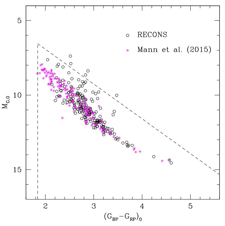
For M-dwarfs, we used The REsearch Consortium On in Appendix A. By means of these selection criteria the initial
Nearby Stars (RECONS5 ) catalogue (Henry et al. 2018), and sample of 179 stars was reduced to 153 stars represented by the
magenta asterisks in Fig. 4.
4
We also compared our reddening E(B − V) with the one calculated
in RAVE and found perfectly consistent results: ∆E(B − V) = (−0.01 ±
0.02). 6
RECONS does not report the effective temperature, but it reports the
5
http://www.recons.org/ spectral type of the stars.
A98, page 5 of 23A&A 653, A98 (2021)
Fig. 4. Left panel: black rectangles represent FGK dwarfs and subgiants from RAVE (see Sect. 3.2, Kunder et al. 2017). Right panel: M-dwarfs
(Henry et al. 2018, open circles) and (Mann et al. 2015, magenta asterisks) catalogues. Dashed lines in both panels show the analytical selection
defined in Sect. 3.3 for the FGK (left) and M stellar samples (right).
3.3. Analytical selection In general, theoretical predictions and observational data
For the selection of M and FGK targets from the Gaia CMD, agree reasonably well. For M-dwarfs, such as those visible in
we then proceeded by defining a set of inequations. The red Figs. 1 and 4, simulated stars appear systematically offset toward
colour limit corresponding to (GBP − GRP )0 = 1.84 was used to larger absolute magnitudes than observations, and appear to span
separate M-dwarfs from FGK dwarfs and subgiants following a smaller colour range. Some differences are also evident among
Pecaut & Mamajek (2013), while the blue colour limit of the the observational samples. Several RECONS stars are intrin-
FGK samples was set at (GBP − GRP )0 = 0.56 corresponding to a sically brighter than the Mann et al. (2015) sample stars. The
spectral type between F4V-F5V according to Pecaut & Mamajek upper absolute luminosity limit of the M sample was set by
(2013). This limit is bluer than the (GBP −GRP )0 = 0.587 proposed performing a linear regression of a 10 Myr solar metallicity
by Pecaut & Mamajek (2013) for F5 stars in order to (partially) isochrone from the Padova database (Bressan et al. 2012), rep-
account for reddening errors. By using TRILEGAL simulations, resented by the blue dashed line in Fig. 1. Considering the the-
we perturbed the reddening correction according to the expected oretical and observational uncertainties, this threshold is a good
reddening uncertainties derived from our map (see Sect. 4), and compromise to include all cool late-type dwarfs at any metal-
estimated the number of contaminants (stars with spectral type licity, including binaries and active stars. At the same time, by
earlier than F5) and targets in narrow colour intervals of 0.05 adopting this limit we are more likely to discard giant stars,
mag. Because our samples are magnitude limited, hotter stars which are expected to be brigher than this limit. To reduce the
are more numerous than cool ones, because they are intrinsically contamination from reddened stars lurking inside our selection
more luminous (see e.g., Fig. 2, left panel). The major source of region we also limited the distance of the stars in the M sam-
contamination comes from massive dwarfs and subgiants of spec- ple to 600 pc. The rationale behind this choice is related to our
tral type earlier than F5. Figure 5 (top panel) shows a colour– limiting magnitude V = 16. Assuming the conversion between
magnitude diagram from Galactic simulations presenting dwarfs Johnson V and Gaia magnitudes in Appendix A, the maximum
and subgiant stars with V < 13 and T eff < 7220 K (i.e. later than distance at which we can detect an unreddened M0 type star with
F0). At the limit of (GBP −GRP )0 = 0.56 (dashed red line) simula- an apparent visual magnitude V = 16 and at the bright limit of our
tions show that we expect a loss of ∼10% of good targets, but an selection (MG,0 = 6.55) is 573 pc. Therefore, any other M-type
inclusion of ∼90% of contaminating stars. Extending the selection star within our selection region cannot be found at a distance of
criteria to bluer colours would increase the number of contaminat- greater than 600 pc. In summary, our adopted selection criteria
ing stars (i.e. stars with spectral type earlier than F5), with negli- are defined as follows:
gible recovery of good targets (bottom panel of Fig. 5). The upper
(GBP − GRP )0 ≥ 1.84
luminosity threshold of FGK subgiants was set to include stars MG,0 > 2.334 (GBP − GRP )0 + 2.259
M sample =
down to log g = 3.5. Such a definition also helps to reduce the
Distance < 600 pc
(2)
contamination from evolved, reddened sources. The lower lumi-
V ≤ 16,
nosity threshold of FGK dwarfs is set at about three magnitudes
below the main sequence to avoid contamination from poten-
0.56 ≤ (GBP − GRP )0 < 1.84
tially spurious sources populating regions of the CMD where no
plausible main sequence dwarf is expected to be found. With MG,0 ≤ 4.1 (GBP − GRP )0 + 5.0
FGK sample =
our selections, distant red giants are excluded by construction (3)
MG,0 ≥ 4.1 (GBP − GRP )0 − 2.2
independently of their reddening and the same holds for white
V ≤ 13.
dwarfs.
A98, page 6 of 23M. Montalto et al.: The all sky PLATO input catalog
By adopting this analytic selection we find that 92% of the stars
whose RAVE parameters are compatible with the selection crite-
ria are included. For the M-dwarf samples we find that 97% (190
out of 195 stars) of the Henry et al. (2018) stars, and 99% (152
out of 153 stars) of the Mann et al. (2015) stars are included in
the selection.
An alternative estimate of the completeness and contami-
nation can be obtained using theoretical models. We used the
same simulations described above in this section to determine
the true positive rate (TPR) and the false positive rate (FPR)
implied by our selection. We distinguished the cases of M and
FGK selected stars. A star is considered a true positive (TP) if
it satisfies inequation (2) for the M sample or inequation (3) for
the FGK sample and the corresponding theoretical constraints
(V < 16, log g > 3.5, and T eff ≤ 3870 K for M sample and
V < 13, log g > 3.5, and 3870 KA&A 653, A98 (2021)
system and the position of the two currently provisionally
defined LOP fields (Nascimbeni et al. 2016). These fields
are centred at Galactic coordinates l = 65◦ , b = 30◦
(RA = 17h :40m :19.265s ; Dec = +39◦ :350 :01.4700 ) for the NPF
and l = 253◦ , b = −30◦ for the SPF (RA = 05h :47m :11.700s ;
Dec = −46◦ :230 :45.3700 ). The definitive choice of the LOP fields,
to be frozen at the latest two years before launch, involves a com-
plex optimisation task to merge several constraints and priorities
of both engineering and scientific nature and will be discussed
in Nascimbeni et al. (in prep.). Nevertheless, the two provisional
fields illustrated in Fig. 9 already satisfy all PLATO requirements
(Sect. 2).
The final all-sky catalogue is named asPIC1.1 and contains
2 675 539 stars. There are 2 378 177 FGK dwarfs and subgiants
(V ≤ 13) and 297 362 M-dwarfs (V ≤16). In Appendix B,
we describe an alternative selection of FGK dwarf and sub-
giant stars based on Johnson B and V photometry, which was
used to construct the first version of this catalogue (asPIC1.0).
In Appendix C, we describe the catalogue content, while in
Appendix D, we present the details of the implementation pro-
cedure that has been adopted to construct asPIC1.1.
Fig. 6. Metallicity distribution of stars selected from the GCS catalogue 4. Reddening and absorption
(Holmberg et al. 2009). The black histogram shows all stars from the Because of the presence of interstellar matter, stars appear redder
catalogue (with T eff < 6500 K) while the red-dashed histogram shows and fainter than they are. This has an impact on the selection of
all stars selected according to asPIC criteria (inequations (2) and (3)).
PLATO targets which is based on the use of photometric quan-
tities like colours and magnitudes, as discussed in Sect. 3. In
particular, as the PLATO samples are magnitude limited, F-type
stars, being intrinsically more luminous are located at larger dis-
tances on average than later type stars, and are therefore the most
affected by reddening. By neglecting the reddening and absorp-
tion correction we estimate that 100% of the stars at the blue
limit of our colour selection (GRP − GBP = 0.56, Eq. (3)) would
be contaminant dwarfs and subgiants (i.e. hotter than spectral
type F5). It is therefore important to account for the impact of
interstellar matter before selecting the target stars.
Different approaches can be considered to determine redden-
ing and extinction. One of the drivers for the choice of the best
approach to follow for the PLATO input catalogue is to consider
that the most important targets lie in the solar neighbourhood.
Considering FGK targets, reddening should be estimated up to a
distance of about 1 kpc.
Figure 10 shows the cumulative distributions of reddening
(left) and HIPPARCOS distances (right) for all stars in the
Geneva-Copenhagen Survey (GCS)7 . The figure shows that 90%
of these stars are within 150 pc and the reddening is E(b −
y) ≤ 0.02 corresponding to E(B − V) ≤ 0.04. In the GCS,
reddening is estimated from the calibration by Olsen (1988)
of the Strömgren photometry intrinsic colour index (b − y).
Fig. 7. Combined selection of FGK and M stars in asPIC1.1. The stated precision is 0.009 mag. The same figure also shows
that around 20% of the stars have negative reddening, and
are too close to allow a reliable reddening determination At
right panel of Fig. 8 shows the distribution of relative distance the small distances of PLATO targets, determining the red-
errors for the different stellar samples. The error on the distance dening on a purely empirical photometric basis is challenging
is calculated from the upper and lower distance limits reported and requires measurements of very high precision. Such esti-
by Bailer-Jones et al. (2018) and is equal to the semi-difference mates can be obtained from measurement of interstellar neu-
of these values. In terms of percentage errors in distance, the tral sodium absorption lines imprinted on spectra of background
median values for the M and FGK stars are 0.6 and 1.6%, respec- stars (e.g., Vergely et al. 2001). Such measurements are best per-
tively. Considering the median distances of the stellar samples formed on early-type stars and extrapolation techniques can be
reported above, this means that M and FGK distances are set used to reconstruct tomographic maps of the local interstellar
with a precision of 0.9 pc and 6.8 pc, respectively. Figure 9 shows
the distribution of the selected FGKM dwarf and subgiant stars 7
We used here the GCSII version (Holmberg et al. 2007) which
across the celestial sphere in a Galactic coordinate reference reports the reddening.
A98, page 8 of 23M. Montalto et al.: The all sky PLATO input catalog Fig. 8. Left: distributions of distances for M (red histogram) and FGK (blue histogram) stars as asPIC1.1. Right: distribution of relative errors on distances in asPIC1.1. Fig. 9. Distribution of asPIC1.1 dwarf and subgiant FGKM stars across the celestial sphere (grey points) in a Galactic coordinates reference system. The plot also shows the position of the two provisional long-duration fields (NPF and SPF). medium in all directions. Such spectroscopic measurements large spectroscopic surveys mitigates this problem), from the have a superior precision than purely photometric estimates, inhomogeneity of the spectroscopic samples adopted and from but the empirical database is still limited (Welsh et al. 2010), the different accuracies and precisions of the effective tempera- and the resulting reddening maps have a limited spatial extent ture determinations. (
A&A 653, A98 (2021)

                                                                            tral types, we used the stellar sample from Casagrande et al.
                                                                            (2010). Effective temperatures reported in this catalogue are
                                                                            calculated using the infrared flux method (IRFM). We cross-
                                                                            matched this sample with Gaia DR2 and considered only stars
                                                                            closer than 40 pc from the Sun. Casagrande et al. (2010) derived
                                                                            the IRFM effective temperatures for all stars with HIPPAR-
                                                                            COS parallaxes and distances ≤70 pc from the Sun assuming
                                                                            they are unaffected by reddening. To be consistent with this
                                                                            choice we assumed that the sample of calibration stars we used
                                                                            (all located within 40 pc) have null reddening. The astromet-
Fig. 10. Left: cumulative distribution of reddening values in GCS.          ric and photometric quality conditions expressed by Eqs. (1)
Right: cumulative distribution of HIPPARCOS distances in GCS. Hori-         and (2) in Arenou et al. (2018) were verified for all the selected
zontal lines denotes the 90th percentile of the cumulative distributions.   stars9 . Our final list comprises 110 stars out of the 423 stars of
                                                                            Casagrande et al. (2010).
                                                                                 For M-dwarfs, we considered the sample of Mann et al.
                                                                            (2015). All the 179 (see Sect. 3.2) stars in the sample are located
                                                                            within 40 pc from the Sun. We also checked that Eqs. (1) and (2)
                                                                            of Arenou et al. (2018) were satisfied, selecting in this way a
                                                                            total of 171 stars. Their effective temperatures were estimated
                                                                            from optical and near-infrared spectra. Finally, for hot stars
                                                                            (T eff > 6510 K), we considered the temperature and colour esti-
                                                                            mates reported in Pecaut & Mamajek (2013).
                                                                                 As shown in Fig. 12, from the resulting sample of 281
                                                                            stars we interpolated a single fifth-order polynomial relating the
                                                                            observed Gaia colour of the calibration stars and their effective
                                                                            temperature. The coefficients of the fit are reported below, and
                                                                            the RMS of the residuals of the fit is equal to 65 K

                                                                            T eff (K) = 9453.14 − 6859.40 (GBP − GRP )0
                                                                                     + 3542.16 (GBP − GRP )20
                                                                                     − 1053.09 (GBP − GRP )30 + 165.635 (GBP − GRP )40
                                                                                     − 10.5672 (GBP − GRP )50 ,                             (4)
Fig. 11. Reddening E(B − V) vs distance for all stars in asPIC1.1.          where the relation is valid for 0.5 < (GBP − GRP ) < 5. Hereafter,
                                                                            we use Eq. (4) as the relation between the intrinsic colour and
Lallement et al. (2018)8 because of its accurate description of             the effective temperature. Using Eq. (4) we obtained a first guess
the local interstellar medium and its overall spatial coverage              of the effective temperature of all asPIC stars. These stars are
which allowed us to determine the reddening for a large fraction            generally located further, at larger distances than the sample of
of PIC stars in a homogeneous way. The 3D reddening map of                  calibration stars, and therefore reddening cannot be neglected.
Lallement et al. (2018) is described in Appendix E. The median                  As reported in Sect. 4, we estimate reddening using the
reddening of asPIC1.1 stars inside the reddening map is equal to            reddening map of Lallement et al. (2018). The customised
E(B − V) = 0.04 and the median uncertainty is σE(B − V) = 0.02.             algorithm described in Sect. E furnishes the interpolated redden-
For the M sample, 99.8% of the stars are contained in the red-              ing E(B − V) for any 3D star position. As input, it requires the
dening map and, for the FGK sample, this figure is 81.8%. For               Galactic longitude l and the Galactic latitude b which are taken
the stars falling outside the map, reddening is calculated up to            directly from the input catalogue along with the distance from
the edge of the map, and then a correction is added, as described           the Bailer-Jones et al. (2018) catalogue.
in Appendix E.1. Figure 11 presents the E(B−V) versus distance
diagram for all stars in asPIC1.1.                                          5.2. Conversion from E(B − V ) to E(GBP − GRP ) and
                                                                                 determination of extinction AG
5. Stellar parameters                                                       The E(B − V) reddening is converted to E(GBP − GRP ) and to the
                                                                            extinction AG in the Gaia G-band as follows:
This section describes the algorithms we used to estimate effec-
tive temperatures, radii, and masses.                                       AG = RG E(B − V),                                               (5)
                                                                            ABP = RBP E(B − V),                                             (6)
5.1. Intrinsic colour-effective temperature relation
                                                                            ARP = RRP E(B − V),                                             (7)
We first determined the relationship between the intrinsic colour
in the Gaia bands and the effective temperature. For FGK spec-              9
                                                                               With the exception of one source, the bright spectroscopic binary
                                                                            HD112758, for which the astrometric condition expressed by Eq. (1)
8
   Very recently Lallement et al. (2019) published an updated version       of Arenou et al. (2018) was not satisfied, but that was kept in the
of the map, which is not included in this version of the catalogue but      sample because it is known to host a low-stellar-mass companion
will be considered in the next version.                                     (Reffert & Quirrenbach 2011).

A98, page 10 of 23
M. Montalto et al.: The all sky PLATO input catalog
adopted isochrone (assuming solar metallicity and solar com-
position), and from the bolometric corrections we calculated
the ratios between the extinction in each band and the redden-
ing E(B − V) as a function of the effective temperature11 . The
results we obtained from our procedure agree well with those of
Casagrande & VandenBerg (2018) in general. Some small differ-
ences are visible, particularly for late-type stars and for the G and
GBP bands which may be explained by differences in the under-
lying model atmospheres, because the Padova group colours
and magnitudes are based on the libraries of stellar spectra of
Castelli & Kurucz (2003), whereas Casagrande & VandenBerg
(2018) used the MARCS library of theoretical stellar fluxes
(Gustafsson et al. 2008).
5.3. Correction for reddening and extinction
The observed GBP −GRP colour and G magnitude were corrected
for reddening and extinction to obtain the intrinsic colour (GBP −
GRP )0 and the intrinsic magnitude G0 :
(GBP − GRP )0 = (GBP − GRP ) − E(GBP − GRP ), (12)
G0 = G − AG . (13)
Fig. 12. Relation between effective temperature T eff and intrinsic colour
(GBP − GRP )0 . The continuous black line denotes our best-fit model 5.4. Effective temperature: the iteration cycle
(Eq. (4)), while the dashed vertical lines denote the limits of validity of
the relation. Coloured dots represent the samples of Casagrande et al. We recalculated the effective temperature using Eq. (4) and the
(2010), Mann et al. (2015), and Pecaut & Mamajek (2013) discussed in new intrinsic colour (GBP − GRP )0 in Eq. (12). We then used
the text in Sect. 5.1. the new effective temperature to estimate the reddening coeffi-
cients (Sect. 5.2) and then a new estimate of the intrinsic colour
where the Gaia extinction coefficients depend on the effective (Sect. 5.3). We then used this to estimate the effective tempera-
temperature as follows ture again. A subsequent iteration lead to effective temperatures
that differ by less than 10 K from last estimate; therefore two
RG = −0.5335 + 12.9373 (T 4 ) − 13.9514 (T 4 )2 iterations were sufficient.
− 13.8012 (T 4 )3 + 40.9902 (T 4 )4 − 23.6648 (T 4 )5 , (8)
RBP = −2.4689 + 59.5802 (T 4 ) − 253.9922 (T 4 ) 2
5.5. Bolometric correction in the G−band, BCG
+ 526.5333 (T 4 ) − 523.9970 (T 4 ) +
3 4
The bolometric correction of the G-band is obtained from the
+ 201.2829 (T 4 ) ,
5
(9) relations given in Andrae et al. (2018):
RRP = 0.0407 + 9.8825 (T 4 ) − 16.8207 (T 4 ) 2 BCG = 6.0 × 10⁻² + 6.731 × 10⁻⁵ ∆T eff − 6.647 × 10−08 ∆T eff
2
+ 9.1283 (T 4 )3 + 2.5051 (T 4 )4 − 2.4158 (T 4 )5 , (10) + 2.859 × 10⁻¹¹ ∆T eff
3
− 7.197 × 10⁻¹⁵ ∆T eff
4
, (14)
and for a temperature interval 4000 K ≤ T eff ≤ 8000 K and
T 4 = 10−4 (T eff ). (11) BCG = 1.749 + 1.977 × 10⁻³ ∆T eff + 3.737 × 10⁻⁷ ∆T eff
2
Such relations were derived using Padova stellar models − 8.966 × 10⁻¹¹ ∆T eff
3
− 4.183 × 10⁻¹⁴ ∆T eff
4
, (15)
(Bressan et al. 2012), assuming solar metallicity, solar compo- for a temperature interval 3300 K ≤ T eff < 4000 K and where
sition, and temperatures within the interval 2500 K < T eff < ∆T eff = T eff − T eff, and T eff, = 5772 K.
7200 K. In particular, we modelled the ratio of the absorption
in a given photometric band to the reddening E(B − V) consid-
ering an unreddened 1 Gyr isochrone, and the same isochrone 5.6. Determination of the absolute magnitude MG,0 and of
reddened using AV = 0.5 mag, where reddening was applied on the absolute luminosity L
a star-by-star basis. We then interpolated apparent magnitudes The intrinsic absolute magnitude MG,0 and the luminosity L were
versus effective temperature on the same temperature grid for calculated as follows:
both the reddened and unreddened isochrones, and calculated
the absorption on each Gaia band as a function of tempera- MG,0 = G0 − 5 log10 d + 5, (16)
ture. In Fig. 13, we show our interpolating relations presented in L
Eqs. (8)–(10) along with the results obtained using the bolomet- = 10−0.4 (MG,0 +BCG −MBOL ) , (17)
ric correction program of Casagrande & VandenBerg (2018)10 . L
In particular, we used this program to calculate the bolomet- where d is the distance of the star in parsecs from
ric corrections for unreddened and reddened stars interpolat- Bailer-Jones et al. (2018) and MBOL = 4.74 and L = 3.828 ×
ing across the grid of log g and effective temperatures of our 1026 W.
Aγ
10
https://github.com/casaluca/bolometric-corrections 11
E(B−V)
= (BCAv=0 −BCAv )
Av
× 3.1, where γ = GBP , G, GRp and Av = 0.5.
A98, page 11 of 23A&A 653, A98 (2021)
Fig. 13. Relations between AG /E(B−V) (left), AGBP /E(B−V) (middle), AGRP /E(B−V) (right) and effective temperature T eff derived with the proce-
dure described in the text (Sect. 5.2). The red lines represent our interpolating relations and the blue lines models from Casagrande & VandenBerg
(2018).
Fig. 14. Relative differences between stellar parameters estimated using asPIC1.1 and theoretical parameters from stellar isochrones in different
metallicity intervals. The rightmost labels of each panel denote the centres of the [M/H] metallicity intervals having a width of ±0.1 dex as also
listed in Table 3.
5.7. Determination of the stellar radius Table 3. Median relative differences (as a percentage) and standard
deviations between asPIC1.1 estimated stellar parameters and theoreti-
We then calculated the stellar radius R from the Stefan- cal stellar parameters in different metallicity intervals.
Boltzmann law:
∆T ∆R ∆M
!−2 s [M/H] T (%) R (%) M (%)
R T eff L
= . (18) −0.9 ≤ [M/H] < −0.7 0.02 ± 0.33 −2.5 ± 0.4 17 ± 9
R T eff, L
−0.7 ≤ [M/H] < −0.5 −0.04 ± 0.30 −1.8 ± 0.3 14 ± 7
The presence of absorption and reddening influences the −0.5 ≤ [M/H] < −0.3 −0.06 ± 0.33 −1.1 ± 0.4 11 ± 6
determination of the stellar radius because it affects both the esti- −0.3 ≤ [M/H] < −0.1 −0.21 ± 0.38 −0.1 ± 0.5 6±5
mation of the effective temperature and of the absolute luminos- −0.1 ≤ [M/H] < 0.1 −0.41 ± 0.36 1.0 ± 0.5 0.5 ± 3.9
ity. Therefore it is important to apply dereddening procedures 0.1 ≤ [M/H] ≤ 0.3 −0.66 ± 0.36 2.6 ± 0.8 −4.1 ± 3.5
like those we describe above. Reddening and absorption have
two opposite and partially compensating effects on the stellar
radius. A more detailed discussion about this point is provided The range of validity is 4780 K ≤ T eff ≤ 10 990 K and
in Appendix F. −0.717 ≤ log (L/L ) ≤ 2.01. This relationship is valid for
dwarfs and subgiant stars.
5.8. Determination of the stellar mass
The stellar mass was determined using the following relation 5.9. Impact of metallicity on the determination of stellar
from Moya et al. (2018): parameters
! ! The procedure used to determine stellar parameters described
M L
log = −0.119 + 2.14 × 10 T eff + 0.1837 × log
−5
. (19) in Sect. 5 does not take into account metallicity because we do
M L not have metallicity measurements for most of our stars. In this
A98, page 12 of 23M. Montalto et al.: The all sky PLATO input catalog
Fig. 15. Distributions of effective temperature (left panel), radius (middle panel), and mass (right panel) for the FGK sample.
section, we estimate the impact that metallicity has on the deter- falling inside its boundaries. For stars falling outside this map,
mination of stellar parameters. We retrieved a grid of isochrones the error on the reddening was assumed equal to twice the error
with age between 7 < log(Age/yr) < 10 in steps of 0.2 dex and on the median reddening of all stars inside the map, which is
metallicity between −1 < [M/H] < 0.3 in steps of 0.1 dex from equal to σ E(B − V) = 0.04 (see also Appendix E). The effective
the Padova stellar database. For each model in the grid, we temperature deduced by the colour–effective temperature rela-
determined the stellar parameters with the procedure described tion was perturbed considering a conservative error of 200 K on
in Sect. 5 and compared them with the theoretical parameters its determination. We performed 100 simulations for each star
reported in the isochrones for six different intervals of metal- and then calculated the errors on the effective temperature, mass,
licity. In particular, we calculated the relative differences ( ∆T T , and radius as the half interval between the 16th and the 84th per-
∆R ∆M centile of the cumulative distribution of the simulated values.
R , M ) between our parameters (T eff,asPIC1.1 , Radius asPIC1.1 ,
MassasPIC1.1 ) and the theoretical parameters (T eff,ISO , RadiusISO , The median value of the effective temperature error is 227 K
MassISO ) (4%), and this value is 0.1 R (7%) for the radius, and 0.1 M
(8%) for the mass.
∆T T eff,asPIC1.1 − T eff,ISO
= , (20)
T T eff,ISO 5.11. Stellar parameter distributions
∆R RadiusasPIC1.1 − RadiusISO
= , (21) In Fig. 15 we present the distributions of effective temperature,
R RadiusISO radius, and mass for the FGK sample. We note that stellar param-
∆M MassasPIC1.1 − MassISO eters have not yet been calculated for the M dwarfs sample. They
= . (22) will be included in the next version of the catalogue.
M MassISO
The results are presented in Fig. 14 and in Table 3. We find
that the effective temperature has a weak dependence on metal- 6. Comparisons
licity with relative differences ranging from −0.6% to 0.02%. We compared stellar parameters and reddening in asPIC1.1 with
The radius presents relative differences of between −2.5% and the values reported in the TIC (Stassun et al. 2019). We used
2.5% while the mass shows the largest relative differences rang- the Candidate Target List v8.01 (CTLv8.01) and cross-matched
ing from −4% to 17%. We note that the mass is also the most it with asPIC1.1 using the Gaia source ID reported in the
uncertain among the theoretical parameters associated to the CTL catalogue. We considered only those stars for which all
isochrones. Both the temperature and the mass relative differ- stellar parameters and the reddening are defined in both cata-
ences are negatively correlated with the metallicity while the logues. We identified 2 022 913 stars in common between the
radius is positively correlated. We also calculated the standard two catalogues. The median differences and the standard devi-
deviations of the relative differences in each metallicity interval. ations of the differences between asPIC1.1 and TIC tempera-
These differences range between 0.3% and 0.4% for the temper- tures, radii, masses, and reddenings are: ∆T eff = (−100 ± 300) K,
ature, between 0.3% and 0.8% for the radius, and between 4% ∆R? = (0.05 ± 0.07) R , ∆M? = (0.05 ± 0.17) M , and
and 9% for the mass. ∆E(B − V) = (−0.002 ± 0.055). We note that the distribution
of stellar masses appears markedly asymmetric with asPIC hav-
5.10. Errors estimate ing a tendency to overestimate the mass with respect to the
TIC. This fact may arise from the different choices adopted for
We determined the errors on stellar parameters using Monte the calibration of stellar masses in the two catalogues. In our
Carlo simulations, perturbing all observing quantities accord- case, we adopted the calibration from Moya et al. (2018) which
ing to their associated errors, and assuming a Gaussian pertur- accounts both for the temperature and absolute luminosity of the
bation. Beyond colours, magnitudes, distances, and reddening, stars, while Stassun et al. (2018, 2019) adopt a calibration based
we also perturbed the bolometric corrections adopting the errors only on the temperatures. The differences between the asPIC1.1
reported by Andrae et al. (2018). The error on the reddening was and TICv8 estimated parameters are shown in the histograms
taken from the reddening map of Lallement et al. (2018) for stars in Fig. 16.
A98, page 13 of 23A&A 653, A98 (2021)
Fig. 16. Distributions of effective temperature, stellar radius, mass, and interstellar reddening differences between asPIC1.1 and CTL.
We then considered the Galactic Archaeology with HER- We also considered the sample of 1111 FGK dwarf
MES (GALAH) survey second data release which contains stars from the HARPS GTO program, homogeneously anal-
342 682 spectroscopically observed stars (Buder et al. 2018). ysed in Adibekyan et al. (2012). We matched the catalogue
We cross-matched GALAH with asPIC1.1 using the Gaia with asPIC1.1 using angular distances (accounting for proper
source ID reported in the catalogue. We found 64 061 matched motions) and found 1102 common sources. The median differ-
sources. We compared the effective temperatures and the ences between the asPIC1.1 and the HARPS effective temper-
log g in GALAH with the asPIC1.1 values. In asPIC1.1 atures and gravities are: ∆T eff = (−70 ± 90) K and ∆ log g =
we report stellar masses (M) and radii (R). The log g is (−0.03 ± 0.15) dex (Fig. 18).
estimated using log g = log M − 2 log R + 4.4374 (Smalley Finally, we compared our parameters with the ones reported
2005). The median differences between the asPIC1.1 and the in the first APOKASC catalogue of spectroscopic and astero-
GALAH effective temperatures and gravities are: ∆T eff = seismic data for dwarfs and subgiants (Serenelli et al. 2017). The
(4 ± 100) K and ∆ log g = (0.1 ± 0.2) dex, as shown in cross-match with asPIC1.1 yielded 385 common stars for which
Fig. 17 all parameters were defined in both catalogues. The analysis
A98, page 14 of 23M. Montalto et al.: The all sky PLATO input catalog
Fig. 17. Distributions of effective temperatures, and stellar gravity differences between asPIC1.1 and GALAH/DR2.
Fig. 18. Distributions of effective temperatures, and stellar gravity differences between asPIC1.1 and the HARPS sample.
was performed both for the SDSS temperature scale and for the Table 4 summarises the results of the comparisons between
spectroscopic temperature scale adopted in the APOGEE Stellar asPIC1.1 and the stellar catalogues considered in this section
Parameters and Chemical Abundances pipeline (ASPCAP). In and we conclude that the average difference between our effec-
the first case, the median differences and the standard deviations tive temperatures and those of the other catalogues is −40 K, the
of the differences between asPIC1.1 and APOKASC tempera- average radius difference is 0.08 R , and the average mass differ-
tures, radii, masses, and gravities are: ∆T eff = (−130 ± 90) K, ence is 0.08 M . Considering the internal errors we estimated in
∆R? = (0.1 ± 0.2) R , ∆M? = (0.1 ± 0.1) M , and ∆ log g = Sect. 5, and adding them in quadrature to the estimated external
(−0.02 ± 0.06), while in the second case: ∆T eff = (90 ± 130) K, errors coming from the comparisons from other catalogues (see
∆R? = (0.1 ± 0.1) R , ∆M? = (0.1 ± 0.1) M , and ∆ log g = above), we conclude that our overall (internal+external) uncer-
(−0.01 ± 0.06) (see also Fig. 19). tainties on the stellar parameters determination is 230 K (4%) for
A98, page 15 of 23A&A 653, A98 (2021)
Fig. 19. Distributions of effective temperatures, stellar radii, masses and gravities differences between asPIC1.1 and APOKASC sample and two
different temperature scales (SDSS, black and ASPCAP, red).
the effective temperatures, 0.13 R (9%) for the stellar radii, and four main public catalogues of exoplanets, and obtain an updated
0.13 M (11%) for the stellar masses. list of the known planets along with their physical and orbital
parameters. In particular, this tool considers the Extrasolar Plan-
ets Encyclopaedia12 , the NASA Exoplanet Archive13 , the Exo-
7. Special target list planets Orbit Database14 , and the Open Exoplanet catalogue15 ,
With the asPIC 1.1 catalogue we also release a special list of 12
http://exoplanet.eu/
objects that consists of all currently known confirmed planet 13
https://exoplanetarchive.ipac.caltech.edu/
hosts included in the asPIC1.1. This list has been constructed 14
http://exoplanets.org/
15
using the Exo-MerCat tool (Alei et al. 2020), which accesses http://www.openexoplanetcatalogue.com/
A98, page 16 of 23M. Montalto et al.: The all sky PLATO input catalog
Table 4. Median differences and standard deviation of the differences between asPIC1.1 and the stellar parameters and interstellar reddening values
from other catalogues.
Catalogue ∆T eff ∆R? ∆M? ∆ log g ∆E(B − V)
(K) (R ) (M ) (dex) (mag)
TIC (CTLv8 ) −100 ± 300 0.05 ± 0.07 0.05 ± 0.17 – −0.002 ± 0.055
GALAH DR2 4 ± 100 – – 0.1 ± 0.2 –
HARPS −70 ± 90 – – −0.03 ± 0.15 –
APOKASC (SDSS) −130 ± 90 0.1 ± 0.2 0.1 ± 0.1 −0.02 ± 0.06 –
APOKASC (ASPCAP) 90 ± 130 0.1 ± 0.1 0.1 ± 0.1 −0.01 ± 0.06 –
each one employing its own cataloguing system. For this rea- edge the financial support of INAF (Istituto Nazionale di Astrofisica), Osser-
son, before obtaining a uniform merging of the objects of inter- vatorio Astronomico di Roma, ASI (Agenzia Spaziale Italiana) under contract
to INAF: ASI 2014-049-R.0 dedicated to SSDC. This work has made use of
est, Exo-MerCat performs a proper discrimination among aliases data from the European Space Agency (ESA) mission Gaia (https://www.
and a standardisation of the different entries provided by the cat- cosmos.esa.int/gaia), processed by the Gaia Data Processing and Anal-
alogues. The list of the known exoplanets is matched with the ysis Consortium (DPAC, https://www.cosmos.esa.int/web/gaia/dpac/
asPIC1.1 catalogue. consortium). Part of this work has been carried out within the framework
The special targets list is a living catalogue: it will be continu- of the National Centre of Competence in Research PlanetS supported by the
Swiss National Science Foundation. E. A. acknowledges the financial support of
ously updated at any new release of asPIC, because the number of the SNSF. C.A. acknowledges support from the KU Leuven Research Council
newly discovered planets will constantly increase over the years, (grant C16/18/005: PARADISE) and from the BELgian federal Science Pol-
not only before but also during the PLATO mission lifetime. icy Office (BELSPO) through PRODEX grants Gaia and PLATO. JMMH is
funded by Spanish State Research Agency grants PID2019-107061GB-C61 and
MDM-2017-0737 (Unidad de Excelencia María de Maeztu CAB). This work
has made use of data from the European Space Agency (ESA) mission Gaia
8. Conclusions (https://www.cosmos.esa.int/gaia), processed by the Gaia Data Pro-
cessing and Analysis Consortium (DPAC, https://www.cosmos.esa.int/
In this paper, we present the asPIC1.1 catalogue, a public all-sky web/gaia/dpac/consortium). Funding for the DPAC has been provided by
catalogue of dwarf and subgiant stars of interest for the PLATO national institutions, in particular the institutions participating in the Gaia Multi-
survey, based on the Gaia DR2 data release. The asPIC cata- lateral Agreement. This paper includes data that has been provided by AAO Data
logue will be fundamental to identifying the best fields for the Central (datacentral.aao.gov.au). The GALAH survey is based on obser-
vations made at the Australian Astronomical Observatory, under programmes
PLATO space mission and the most promising targets, analysing A/2013B/13, A/2014A/25, A/2015A/19, A/2017A/18. We acknowledge the tra-
the instrumental performances as well as planning and optimis- ditional owners of the land on which the AAT stands, the Gamilaraay people, and
ing ground-based follow-up studies. This catalogue also repre- pay our respects to elders past and present. The full catalogue of known plan-
sents a valuable resource for the construction of stellar samples ets/candidates retrieved by Exo-MerCat is registered as a Virtual Observatory
optimised for the search of transiting planets. resource and it is available on TOPCAT (Taylor 2005). It can be also provided
and customized by a dedicated User Interface, available from a public GitHub
The catalogue includes a total of 2 675 539 stars among repository (https://gitlab.com/eleonoraalei/exo-mercat-gui). Some
which 2 378 177 are FGK dwarfs and subgiants and 297 362 are of the results in this paper have been derived using the HEALPix (Górski et al.
M-dwarfs. The median distance of FGK stars in our sample is 2005) package.
428 pc and that for M dwarfs is 146 pc.
We also show that our selection criteria do not bias the sta-
tistical distribution of metallicities, and we analyse the impact References
that metallicity has on the derivation of stellar parameters. We
Adibekyan, V. Z., Sousa, S. G., Santos, N. C., et al. 2012, A&A, 545, A32
derived the reddening of our targets and developed an algo- Alei, E., Claudi, R., Bignamini, A., & Molinaro, M. 2020, Astron. Comput., 31,
rithm to infer stellar fundamental parameters from astrometric 100370
and photometric measurements. We show that the overall (inter- Andrae, R., Fouesneau, M., Creevey, O., et al. 2018, A&A, 616, A8
nal+external) uncertainties on the stellar parameters determined Arenou, F., Luri, X., Babusiaux, C., et al. 2018, A&A, 616, A17
Bailer-Jones, C. A. L., Rybizki, J., Fouesneau, M., Mantelet, G., & Andrae, R.
by our analysis are ∼230 K (4%) for the effective temperatures, 2018, AJ, 156, 58
∼0.1 R (9%) for the stellar radii, and ∼0.1 M (11%) for the Binney, J., Burnett, B., Kordopatis, G., et al. 2014, MNRAS, 437, 351
stellar masses. We also release a special target list containing all Borucki, W. J., Koch, D., Basri, G., et al. 2010, Science, 327, 977
known planet hosts cross-matched with our catalogue. Bressan, A., Marigo, P., Girardi, L., et al. 2012, MNRAS, 427, 127
Brown, T. M., Latham, D. W., Everett, M. E., & Esquerdo, G. A. 2011, AJ, 142,
112
Acknowledgements. The authors are grateful to the referee, Keivan Stassun, Bryson, S., Coughlin, J., Batalha, N. M., et al. 2020, AJ, 159, 279
for reading the manuscript and providing constructive comments and sugges- Buder, S., Asplund, M., Duong, L., et al. 2018, MNRAS, 478, 4513
tions. This work presents results from the European Space Agency (ESA) Casagrande, L., Ramírez, I., Meléndez, J., Bessell, M., & Asplund, M. 2010,
space mission PLATO. The PLATO payload, the PLATO Ground Segment and A&A, 512, A54
PLATO data processing are joint developments of ESA and the PLATO Mis- Casagrande, L., & VandenBerg, D. A. 2018, MNRAS, 479, L102
sion Consortium (PMC). Funding for the PMC is provided at national lev- Castelli, F., & Kurucz, R. L. 2003, in Modelling of Stellar Atmospheres, eds.
els, in particular by countries participating in the PLATO Multilateral Agree- N. Piskunov, W. W. Weiss, & D. F. Gray, 210, A20
ment (Austria, Belgium, Czech Republic, Denmark, France, Germany, Italy, Chen, B. Q., Huang, Y., Yuan, H. B., et al. 2019, MNRAS, 483, 4277
Netherlands, Portugal, Spain, Sweden, Switzerland, Norway, and United King- Corso, A. J., Tessarolo, E., Baccaro, S., et al. 2018, Opt. Express, 26, 33841
dom) and institutions from Brazil. Members of the PLATO Consortium can be Deleuil, M., Meunier, J. C., Moutou, C., et al. 2009, AJ, 138, 649
found at https://platomission.com/. The ESA PLATO mission website Evans, D. W., Riello, M., De Angeli, F., et al. 2018, A&A, 616, A4
is https://www.cosmos.esa.int/plato. We thank the teams working for Fressin, F., Torres, G., Charbonneau, D., et al. 2013, ApJ, 766, 81
PLATO for all their work. M. M., G. P., V. N., V. G., L. P., S. D., S. O., S. B., Gaia Collaboration (Prusti, T., et al.) 2016, A&A, 595, A1
R. C., L. M., I. P. acknowledge support from PLATO ASI-INAF agreements Gaia Collaboration (Brown, A. G. A., et al.) 2018, A&A, 616, A1
n.2015-019-R0-2015 and n. 2015-019-R.1-2018. We would like to acknowl- Gaia Collaboration (Brown, A. G. A., et al.) 2021, A&A, 649, A1
A98, page 17 of 23You can also read