SPINS, A PIPELINE FOR MASSIVE STELLAR PARAMETER INFERENCE
←
→
Page content transcription
If your browser does not render page correctly, please read the page content below
Astronomy & Astrophysics manuscript no. article                                                                                       c ESO 2020
                                               September 2, 2020

                                                           SPInS, a pipeline for massive stellar parameter inference
                                                              A public Python tool to age-date, weigh, size up stars, and more
                                                                                                     Y. Lebreton1, 2 and D. R. Reese1

                                                     1
                                                         LESIA, Observatoire de Paris, Université PSL, CNRS, Sorbonne Université, Université de Paris, 5 place Jules Janssen, 92195
                                                         Meudon, France
                                                         e-mail: yveline.lebreton@obspm.fr, daniel.reese@obspm.fr
                                                     2
                                                         Univ Rennes, CNRS, IPR (Institut de Physique de Rennes) - UMR 6251, F-35000 Rennes, France
arXiv:2009.00037v1 [astro-ph.SR] 31 Aug 2020

                                                     Received 8 June 2020 ; accepted July 2020

                                                                                                                  ABSTRACT

                                                     Context. Stellar parameters are required in a variety of contexts, ranging from the characterisation of exoplanets to Galactic archaeol-
                                                     ogy. Among them, the age of stars cannot be directly measured, while the mass and radius can be measured in some particular cases
                                                     (e.g. binary systems, interferometry). More generally, stellar ages, masses, and radii have to be inferred from stellar evolution models
                                                     by appropriate techniques.
                                                     Aims. We have designed a Python tool named SPInS. It takes a set of photometric, spectroscopic, interferometric, and/or asteroseismic
                                                     observational constraints and, relying on a stellar model grid, provides the age, mass, and radius of a star, among others, as well as
                                                     error bars and correlations. We make the tool available to the community via a dedicated website.
                                                     Methods. SPInS uses a Bayesian approach to find the probability distribution function of stellar parameters from a set of classical
                                                     constraints. At the heart of the code is a Markov Chain Monte Carlo solver coupled with interpolation within a pre-computed stellar
                                                     model grid. Priors can be considered, such as the initial mass function or stellar formation rate. SPInS can characterise single stars or
                                                     coeval stars, such as members of binary systems or of stellar clusters.
                                                     Results. We first illustrate the capabilities of SPInS by studying stars that are spread over the Hertzsprung-Russell diagram. We then
                                                     validate the tool by inferring the ages and masses of stars in several catalogues and by comparing them with literature results. We show
                                                     that in addition to the age and mass, SPInS can efficiently provide derived quantities, such as the radius, surface gravity, and seismic
                                                     indices. We demonstrate that SPInS can age-date and characterise coeval stars that share a common age and chemical composition.
                                                     Conclusions. The SPInS tool will be very helpful in preparing and interpreting the results of large-scale surveys, such as the wealth
                                                     of data expected or already provided by space missions, such as Gaia, Kepler, TESS, and PLATO.
                                                     Key words. Stars: fundamental parameters – Methods: numerical – Hertzsprung-Russell and C-M diagrams – Asteroseismology

                                               1. Introduction                                                             lar parameters acute. With Gaia (Gaia Collaboration et al. 2018)
                                                                                                                           and large spectroscopic surveys being conducted in parallel (see
                                               Stellar ages, masses, and radii (hereafter stellar parameters) are          details and references in Sect. 2 of Miglio et al. 2017), the
                                               indispensable basic inputs in many astrophysical studies, such as           number of stars with precise astrometry, kinematics, and abun-
                                               the study of the chemo-kinematical structure of the Milky Way               dances will increase by more than three orders of magnitude.
                                               (i.e. Galactic archaeology), exoplanetology, and cosmology. In-             With high-precision photometry space-borne missions such as
                                               deed, stellar parameters have long been used to answer questions            CoRoT (Baglin et al. 2006), Kepler (Borucki et al. 2010), K2
                                               on how stars populating the different structures, that is the discs,        (Howell et al. 2014), TESS (Ricker et al. 2015), and in the fu-
                                               bulge, and halo, in our Galaxy were formed and evolve, and to               ture PLATO (Rauer et al. 2014), thousands of exoplanets have
                                               decipher in-situ formation, migration, and mergers. In this con-            been and will be discovered. For planetary host stars of F, G, K
                                               text, stellar parameters are the basis of stellar age-metallicity and       spectral type on the main sequence or on the red giant branch,
                                               age-velocity relations, the stellar initial mass function (IMF), or         it is and will be possible to extract the power spectrum of their
                                               the stellar formation rate (SFR) [see Haywood (2014) for a re-              solar-like oscillations from the observed light curve, providing
                                               view]. Also, the ages of the oldest stars provide a robust lower            asteroseismic constraints to their modelling. Asteroseismology,
                                               limit to the age of the Universe. Recently, with the discovery of           therefore, will give access to precise and accurate masses, radii,
                                               several thousands of exoplanetary systems, it has become evi-               and ages for these stars (see e.g. Lebreton & Goupil 2014; Silva
                                               dent that no characterisation of the internal structure and evolu-          Aguirre et al. 2015). However, for cold M-type stars, which are
                                               tionary stage of planets is possible without a precise determina-           optimal candidates for hosting habitable planets, the availabil-
                                               tion of the radius, mass, and age of the host stars (see e.g. Rauer         ity of asteroseismic constraints is less probable. In this context,
                                               et al. 2014).                                                               to fully exploit these rich data harvests and ensure scientific re-
                                                    Today, the availability of observations from large-scale as-           turns, we need modern numerical tools that are able to infer the
                                               trometric, photometric, spectroscopic, and interferometric sur-             stellar parameters of very large samples of stars.
                                               veys has made the demand for very precise and accurate stel-
                                                                                                                                                                      Article number, page 1 of 16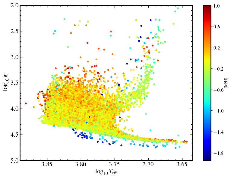
A&A proofs: manuscript no. article

    Soderblom (2010) reviewed the various methods that can be          to perform a full asteroseismic analysis and can estimate stellar
applied to age-date a star, pointing out that a given method (i) in    parameters from two sets of observations: classical data and de-
most cases is only applicable to a limited range of stellar masses     tailed asteroseismic constraints (individual oscillation frequen-
or evolutionary stages, (ii) can provide either absolute or rela-      cies or a combination thereof). While AIMS is essentially an as-
tive ages, and (iii) is sometimes only applicable to very small        teroseismic tool, SPInS is not intended to handle detailed seismic
stellar samples. Moreover, the precision and accuracy tightly de-      data but rather focuses on classical or mean observed stellar data
pend on the age-dating method. Here, we focus on the so-called         (these will be explained in the following sections). This greatly
isochrone placement method (Edvardsson et al. 1993) that has           simplifies the procedure with a substantial gain in computational
long been used for age-dating and weighing stars in extended re-       time and occupied disc space. In particular, SPInS only uses the
gions of the Hertzsprung-Russell (hereafter H–R) diagram. This         standard outputs of stellar evolution models and does not need
method only requires having stellar evolutionary models avail-         to be provided with the detailed calculations of the oscillation
able and is rather straightforward. It can provide ages and masses     spectrum of the models.
when other more powerful techniques, such as asteroseismology,              SPInS was initially created in 2018 to be used in hands-on
are not applicable. It can also serve as a reference when several      sessions during the 5th International Young Astronomer School
age-dating methods are applicable. The precision depends on the        held in Paris8 . The goal of SPInS is to estimate stellar ages and
star’s mass and evolutionary state. Basically, the method consists     masses, as well as other properties and their error bars, in a prob-
in inferring the age and mass of an observed star with measured        abilistic manner. This tool takes in a grid of stellar evolution-
effective temperature, absolute magnitude, and metallicity (here-      ary tracks and applies a Monte Carlo Markov Chain (MCMC)
after classical data) or any proxy for them, by looking for the        approach in combination with a multidimensional interpolation
theoretical stellar model that best fits the observations (e.g. Ed-    scheme in order to find which stellar model(s) best reproduce(s)
vardsson et al. 1993; Ng & Bertelli 1998). The adjustment can          the observed luminosity L? (or any proxy for it, such as the
be performed in different ways. The simplest way to proceed is         absolute magnitude in a given band Mb,? ), effective tempera-
to select the appropriate isochrone by a χ2 -minimisation, that is     ture T eff,? (or any colour index), and observed surface metal
by searching among the isochrone points which one is closest           content [M/H]. The latter can be replaced or complemented by
to the star’s location, in the related parameter space (see e.g. Ng    other data derived from observations, such as the surface gravity
& Bertelli 1998). However, the selection of the right isochrone        log g, the mass or radius, or both (for stars in eclipsing, spectro-
may be difficult in regions of the H–R diagram where they have         scopic, visual binaries, or with interferometric measurements),
a complex shape. In such regions, the evolutionary state of the        or asteroseismic parameters (the frequency at maximum power,
star cannot be determined unambiguously and the star’s posi-           the mean large frequency separation inferred from the pressure-
tion can equally be fitted with several isochrone points of differ-    mode power spectrum, etc.). The advantage of this approach is
ent ages, masses, and metal contents. To improve the age-dating        that it provides a full probability distribution function (hereafter
procedure, Pont & Eyer (2004) proposed a Bayesian approach             PDF) for any stellar parameter to be inferred, thereby account-
that, by adding prior information about the stellar and Galac-         ing for multiple solutions when present. It also allows the user to
tic properties, allows the procedure to choose the most proba-         incorporate in the calculation various priors (i.e. a priori assump-
ble age. The technique has been refined and improved by Jør-           tions), such as the initial mass function (IMF), the stellar forma-
gensen & Lindegren (2005), da Silva et al. (2006), von Hippel          tion rate (SFR), or the metallicity distribution function (MDF).
et al. (2006), Takeda et al. (2007), Hernandez & Valls-Gabaud          SPInS can be used in two operational modes: characterisation of
(2008), and Casagrande et al. (2011), for the earlier papers, and      a single star or characterisation of coeval groups, including bina-
reviewed by Valls-Gabaud (2014) and von Hippel et al. (2014).          ries and stellar clusters. SPInS is mostly written in Python with a
In this context, the work by da Silva et al. (2006) gave birth to      modular structure to facilitate contributions from the community.
the PARAM1 web interface for the Bayesian estimation of stel-          Only a few computationally intensive parts have been written in
lar parameters. Then, a few stellar age-dating public codes with       Fortran in order to speed up calculations.
different specificities were made public: BASE-92 that allows the           The paper is organised as follows. In Sect. 2, we explain the
users to infer the properties of stellar clusters and their members,   Bayesian approach used in SPInS. In Sect. 3, we present some
including white dwarfs (von Hippel et al. 2006), UniDAM3 that          results obtained with SPInS for a set of fictitious stars with par-
can be used to exploit large stellar surveys (Mints et al. 2019),      ticularly noticeable locations in the H–R diagram. In Sect. 4,
stardate4 that considers constraints from gyrochronology (Angus        we compare results obtained by SPInS with those derived by
et al. 2019), and MCMCI5 that is dedicated to the characterisa-        Casagrande et al. (2011). In Sect. 5, we show inferences on prop-
tion of exoplanetary systems (Bonfanti & Gillon 2020).                 erties of stars observed either in interferometry or in asteroseis-
    In this work, we present and make public6 a new tool based         mology. In Sect. 6, we use SPInS to study coeval stars belonging
on Python and Fortran, named SPInS (standing for Stellar Pa-           to a binary system and an open cluster. Finally, we draw some
rameters Inferred Systematically). SPInS is a modified version         conclusions in Sect. 7.
of the AIMS (Asteroseismic Inference on a Massive Scale)
pipeline7 . The AIMS code has been described and evaluated by
Lund & Reese (2018) and Rendle et al. (2019). AIMS is able             2. Description of the SPInS code
1                                                                      2.1. Overview
  PARAM: http://stev.oapd.inaf.it/cgi-bin/param
2
  BASE-9: https://github.com/BayesianStellarEvolution                  SPInS uses a Bayesian approach to find the PDF of the stellar
3
  UniDAM: http://www2.mps.mpg.de/homes/mints/unidam.                   parameters from a set of observational constraints. At the heart
html                                                                   of the code is a MCMC solver based on the Python EMCEE
4
  stardate: https://github.com/RuthAngus/stardate                      package (Foreman-Mackey et al. 2013) coupled to interpolation
5
  MCMCI: https://github.com/dfm/exoplanet
6                                                                      8
  SPInS: https://gitlab.obspm.fr/dreese/spins                             International School organised by the Paris Doctoral School of As-
7
  AIMS:        https://lesia.obspm.fr/perso/daniel-reese/              tronomy & Astrophysics, see https://gaiaschool.wixsite.com/
spaceinn/aims/                                                         gaia-school2018.

Article number, page 2 of 16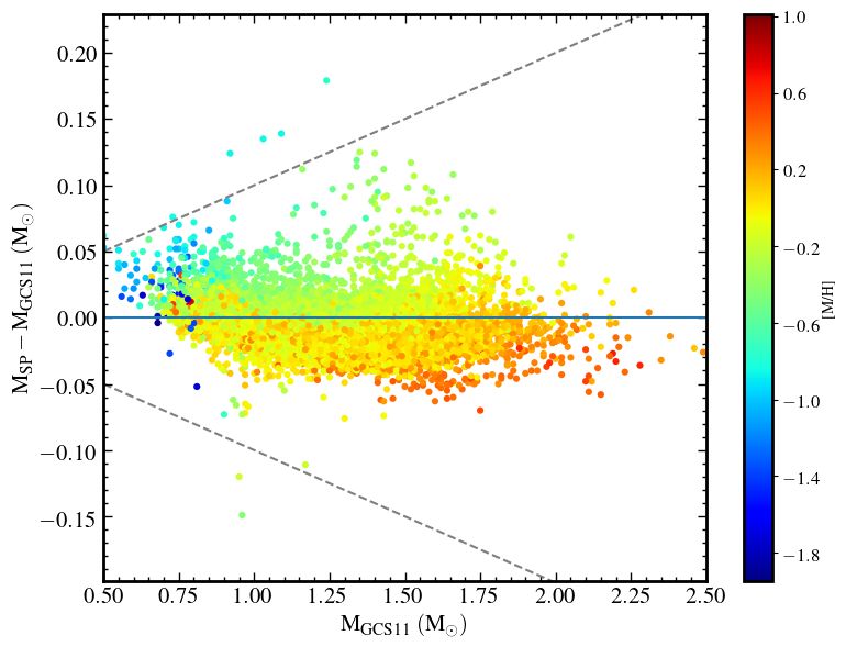
Y. Lebreton and D. R. Reese: SPInS, a pipeline for massive stellar parameter inference
within a pre-computed grid of stellar models. This allows SPInS 2.2.2. Stellar formation rate
to produce a sample of interpolated models representative of the
underlying posterior probability distribution. We recall that the We restrict our working age domain to an upper limit of 13.8
posterior probability distribution can be obtained from the priors Gyr, that is roughly the age of the Universe, and we used the
and the likelihood via Bayes’ theorem: following uniform truncated stellar formation rate (SFR):
P(O|θ)P(θ) (
for τ1 = 0 ≤ τ ≤ τ2 = 13.8 Gyr ,
P(θ|O) = , (1) λ(τ) =
1
(6)
P(O) 0 elsewhere.
where O are the observational constraints and θ the model pa- This translates into a prior on the age of a star.
rameters. In other words, this theorem provides a way of calcu-
lating the probability distribution for model parameters given a
set of observational constraints, as represented by the likelihood 2.2.3. Metallicity distribution function
function P(O|θ), and priors P(θ). The next two sections will deal We assume that the metallicity measurements are or will be
with these two terms in more detail. available for the stars we want to age-date. Therefore, we do
not introduce an a priori assumption on what their metallicity
2.2. The priors should be (see the discussion in Jørgensen & Lindegren 2005).
Thus, by default, we adopt a flat prior on the metallicity [M/H]
The priors represent our a priori knowledge of how the model distribution function (MDF).
parameters should behave. For instance, one expects a higher However, any prior on the MDF can be introduced into
number of low-mass stars than high-mass stars, and this can be SPInS. As an example, in Sect. 4, we introduced the prior
expressed as a prior on the mass with a higher probability at adopted by Casagrande et al. (2011) and given in their Ap-
low mass values. As described in the following subsections, the pendix A to correct for metallicity biases found in the Geneva-
priors will apply to the following stellar parameters given that Copenhagen Survey.
we will be working with BaSTI stellar model grids (Pietrinferni
et al. 2004, 2006): mass, age, and metallicity. Of course, the
choice of model parameters that are included in the priors de- 2.3. The likelihood function
pends on the parameters that describe the grid being used with The likelihood function is used to introduce observational con-
SPInS. straints. Typically, these include constraints on classic observ-
ables, such as the luminosity, effective temperature, and metal-
2.2.1. Initial mass function
licity. However, as will be shown in the following, constraints on
other observables may be used, such as the absolute magnitude
The initial mass function (IMF) was first introduced by Salpeter in any photometric band, colour indices, asteroseismic indices,
(1955). It provides a convenient way of parametrising the rel- radius, and whatever parameters are available with the grid of
ative numbers of stars as a function of their mass in a stellar models being used with SPInS (as described in Sect. 2.5). These
sample (see e.g. the review by Bastian et al. 2010). constraints take on the form of probability distributions on the
The number dN(m) of stars formed in the mass interval value of the parameter. This leads to the following formulation
[m, m + dm] reads dN(m) = ξ(m)dm where ξ(m) is the IMF. for the likelihood function:
SPInS can handle two forms of the IMF: a one-slope version Y
that reads P(O|θ) = Pi (Oi |θ), (7)
i
−α
ξ(m) ∝ mmH for m0 < m/M ≤ mmax , (2) where the Pi represent the probability distributions on individ-
ual parameters resulting from the observational constraints, and
and a two-slopes version, Oi the values of those parameters obtained for a given set of
−α1 model parameters θ. The probability distributions Pi are typi-
m
for mH < m/M ≤ m0 , cally normal distributions although other options are available
ξ(m) ∝
mH
(3) with SPInS.
m0 −α1 m −α2
for m0 < m/M ≤ mmax .
mH m0
The one parameter version (Eq. 2) is related to the IMF intro- 2.4. Variable changes
duced by Salpeter (1955) with the following parameter, One of the features of SPInS is to allow variable changes. For
√
α = 2.35 for m0 = 0.40 < m/M ≤ mmax = 10. (4) instance, one may have observational constraints on L rather
than L or may have a prior on log10 M rather than M. SPInS
The two-parameters version (Eq. 3) can be used to implement allows such variable changes for a handful of elementary func-
the canonical IMF from Kroupa et al. (2013, section 9.1) which tions. Of course, such changes need to be taken into account in
is suitable for stars in the solar neighbourhood. In that case, a self-consistent way. In other words, the underlying probability
distribution should not be altered. Accordingly, variable changes
on observed parameters are treated differently than those on
α1 = 1.30 ± 0.30 for mH = 0.07 < m/M ≤ m0 = 0.50,
(
(5) model parameters. To understand this, we recall the relationship
α2 = 2.30 ± 0.36 for m0 = 0.50 < m/M ≤ mmax = 150.
between probability functions after a change of variables:
Any other form of the IMF can easily be added to the SPInS dy
program. PX (x) = PY (y(x)) . (8)
dx
Article number, page 3 of 16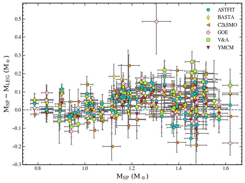
A&A proofs: manuscript no. article

We then introduce this relation into Bayes’ theorem and assume                  of the number abundance of α-elements (i.e. formed by α-
for simplicity that there is a single observed parameter and a                  capture thermonuclear reactions) with respect to iron and ref-
single model parameter. We then assume the prior and likelihood                 erenced to the solar value ([α/Fe] = 0.0). These grids are
function apply to f (θ) and g(O), respectively, instead of θ and O.             described in Pietrinferni et al. (2006).
This leads to:
                                                                              For each evolutionary track in the BaSTI database, the vari-
                          dg(O)               d f (θ)
              P(g(O)|θ)    dO     P( f (θ))     dθ                        ation of the luminosity, effective temperature, absolute Mb mag-
P(θ|O) =                                                                  nitude, and colour indices are provided as a function of the age
                                  dg(O)
                       P(g(O))     dO                                     and mass of the model star for several photometric systems. We
              P(g(O)|θ)P( f (θ)) d f (θ)                                  here use the tracks given in the Johnson-Cousins system which
         =                               .                          (9)   provide MV , and (B − V), (U − B), (V − I), (V − R), (V − J), (V −
                  P(g(O))          dθ                                     K), (V − L), (H − K) colours, but other photometric systems are
As can be seen, a change of variables on an observed constraint           available in the BaSTI database. All these quantities can be used
does not lead to any modification to the way the probability is           indifferently in SPInS.
calculated because the corrective terms cancel out. In contrast,              In addition, we considered four quantities that can be in-
applying a prior to a different variable than the one used in the         ferred from BaSTI models straightforwardly: the photospheric
                                                                          radius R? calculated from Stefan Boltzmann’s law, the surface
grid requires multiplying by the term d dθf (θ)
                                                . SPInS accordingly       gravity
takes this term into account using analytic derivatives of the ele-
mentary functions used in the variable change.                                  GM?
                                                                          g=         ,                                                     (10)
                                                                                 R2?
2.5. Grids of stellar models                                              (or its decimal logarithm log g), and the frequency at maximum
SPInS can easily include any set of evolutionary tracks or                amplitude νmax,sc and the mean large frequency separation of
isochrones available in the literature or calculated by the user. In      pressure modes h∆νisc expressed in asteroseismic scaling rela-
this work, we used the BaSTI stellar evolutionary tracks avail-           tions. The latter read,
able at http://albione.oa-teramo.inaf.it/index.html                                                !−1/2    !−2
                                                                          νmax,sc
                                                                                         !
                                                                                     M? T eff, ?         R?
and described in Pietrinferni et al. (2004, 2006). We chose to use                =                             ,                     (11)
these data rather than more recent ones in order to make com-              νmax,     M      T eff,       R
parisons with previous works.
                                                                          and
    In the BaSTI database, many sets of stellar tracks, all in the
mass range M ∈ [0.5M , 10M ], are available. These models                 h∆νisc   M?
                                                                                          !1/2
                                                                                                 R?
                                                                                                      !−3/2
are well-suited to age-dating stars of different kinds: they cover               =                            ,                            (12)
                                                                          h∆νi     M             R
evolutionary stages running from the zero-age main sequence
(we do not use here the additional pre-main sequence grid pro-            and are explained in Brown et al. (1994); Kjeldsen & Bedding
vided for a narrower range of mass) to advanced stages, includ-           (1995); Belkacem et al. (2011). In Eqs. 10, 11, and 12, G is the
ing the red-giant and horizontal branches, and a metal abun-              gravitational constant, M? the mass of the star, T eff, = 5777 K,
dance range Z ∈ [0.0001, 0.04], where Z is expressed in mass              the subscript ‘sc’ stands for scaling, and νmax, = 3090 µHz and
fraction. This interval of Z-values corresponds to number abun-           h∆νi = 135.1 µHz are the solar values in Huber et al. (2011).
dances of metals relative to hydrogen [M/H] ∈ [−2.27, +0.40],             In the following, νmax,sc and h∆νisc will be referred to as seismic
where [M/H] = log(Z/X) − log(Z/X) and X is the hydrogen                   indices.
mass fraction. The value of (Z/X) depends on the solar mixture
under consideration. GN93’s solar mixture (Grevesse & Noels
1993) has a value (Z/X) = 0.0245.                                         2.6. Interpolation in the grids
    On the BaSTI website, the following grids are available:              As was the case for the AIMS code, SPInS uses a two-step
                                                                          process for interpolation. This then allows the MCMC algo-
 – Canonical grid: it corresponds to standard stellar models              rithm to randomly select any point within the relevant parameter
   that do not include gravitational settling, radiative acceler-         space. The first part of the interpolation concerns interpolation
   ations, convective overshooting, rotational mixing, but oth-           between evolutionary tracks. The second part concerns interpo-
   erwise are based on recent physics, as detailed in Pietrinferni        lation along the tracks, that is as a function of age. These are
   et al. (2004). The models are based on GN93’s solar mixture.           described in the following subsections.
 – Non-canonical grid: the difference with the canonical grid
   is that models in this grid account for core convective over-
   shooting during the H-burning phase which may have a non-              2.6.1. Interpolation between evolutionary tracks
   negligible impact on age. As described in Pietrinferni et al.          Interpolation between evolutionary tracks amounts to interpo-
   (2004), in these models, convective mixing is extended over            lating in the parameter space defined by the grid parameters,
   0.2 pressure scale-heights above the Schwarzschild’s core for          excluding age. In this parameter space, each track corresponds
   a stellar mass higher than 1.7 M , no overshooting is consid-          to a single point. As a first step, a Delaunay tessellation is car-
   ered for a mass lower than 1.1 M , and a linear variation is           ried out for this set of points via the Qhull package9 (Barber
   assumed in-between.                                                    et al. 1996) as implemented in SciPy10 . As a result, the parame-
 – α-enhanced model grids (both canonical and non-canonical):             ter space is subdivided into a set of simplices (i.e. triangles in two
   their element mixture corresponds to a metal distribution
   typical of the Galactic halo and bulge stars, with [α/Fe] =             9
                                                                               http://www.qhull.org/
   +0.4, where [α/Fe] is the decimal logarithm of the ratio               10
                                                                               https://www.scipy.org/

Article number, page 4 of 16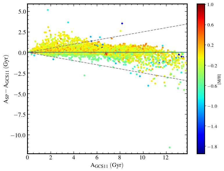
Y. Lebreton and D. R. Reese: SPInS, a pipeline for massive stellar parameter inference

dimensions, tetrahedra in three dimensions, etc.). Then, for any
point within the convex hull of the tessellation, SPInS searches
for the simplex which contains the point and carries out a lin-
ear barycentric interpolation on the simplex. The advantage of
such an approach is that the grid of stellar models can be com-
pletely unstructured, thus providing SPInS with a greater degree
of flexibility. Furthermore, fewer tracks are linearly combined
during the interpolation process thus potentially saving compu-
tation time compared to multilinear interpolation in Cartesian
grids of the same number of dimensions.

2.6.2. Interpolation along evolutionary tracks

The second part of the interpolation focuses on age interpolation
along evolutionary tracks. Interpolation along a track is achieved
by simple linear interpolation between adjacent points thus lead-
ing to piecewise affine functions for the various stellar param-
eters as a function of age. What is more difficult is combining           Fig. 1. Schematic plot illustrating how age interpolation works in
age interpolation with interpolation between tracks. As opposed           SPInS. The two solid lines correspond to two neighbouring stellar evo-
to AIMS, SPInS uses two variables for the age: the physical age           lutionary tracks which are involved in the interpolation. The horizon-
and a dimensionless age parameter. The purpose of the age pa-             tal hatch marks indicate that the interpolation takes place horizontally
rameter is to provide equivalent evolutionary stages on differ-           (i.e. models with the same age parameter rather than physical age are
ent tracks for the same value of this parameter. This then allows         linearly combined). The dotted line shows the interpolated track. The
SPInS to combine models at the same evolutionary stage when               vertical blue dashed line corresponds to the target age and the yellow
interpolating between tracks thus improving the accuracy of the           dot to the interpolated model.
interpolation. Nonetheless, from the point of view of the MCMC
algorithm, it is the physical age which is relevant, that is to say
the MCMC algorithm will sample the physical age (thus bypass-
ing the need for a corrective term as in Eq. 8). This is particularly     ors is applied to the model parameters for each star. For common
important when fitting multiple coeval stars, that is with a com-         parameters, the prior is only applied once, unless the user specif-
mon physical age. Hence, SPInS is constantly going back and               ically configures SPInS to apply it to each star (which amounts
forth between these two age variables.                                    to raising the prior to the power nstars , where nstars is the number
    Sampling as a function of physical age while interpolating in         of stars). Hence, the overall posterior probability is obtained as
terms of the age parameter is not straightforward as illustrated          the product of the likelihood functions and priors applied to the
in Fig. 1. In the plot, the interpolated track is halfway between         parameters of each star apart from those of the common param-
the two original tracks for fixed values of the age parameter (al-        eters which are only applied once. Finally, for stellar samples
though, SPInS can, of course, also interpolate using other inter-         sharing the same age, an isochrone file may be produced cover-
polation coefficients). The same is not true for fixed stellar ages:      ing the whole mass interval spanned by the stellar models used
the interpolated track is not halfway between the original tracks         by SPInS. Fitting multiple stars is advantageous as it can lead
for fixed stellar ages, as can be seen for instance with the verti-       to tighter constraints on common parameters (e.g. Jørgensen &
cal dashed line at the target age. Hence, one cannot simply find          Lindegren 2005).
the age parameters on the original tracks for the target stellar
age and interpolate between these to obtain the age parameter
of the interpolated model. One solution would be to interpolate           2.8. Typical calculation times
the entire track and then search for the age parameter directly
                                                                          Computation times depend on a number of factors such as
on it. This is, however, not the most efficient approach computa-
                                                                          the number of stars being fitted, nstars , and the number of
tionally as most of the track is not needed and would probably
                                                                          dimensions of the grid (excluding age), ndim , as well as on
considerably slow down SPInS given that this operation would
                                                                          various MCMC parameters such as the number of iterations
need to be performed for each set of parameters tested by the
                                                                          (both burn-in and production), niter , the number of walk-
MCMC algorithm. The solution implemented in SPInS consists
                                                                          ers, nwalk , and the number of temperatures if applying par-
in a dichotomic search as a function of the age parameter com-
                                                                          allel tempering, ntemp . Typical computation times for individ-
bined with a direct resolution once the interval is small enough
                                                                          ual stars, (nstars , ndim , niter , nwalk , ntemp ) = (1, 2, 400, 250, 10),
to only contain a single affine section of the interpolated track.
                                                                          is of the order of 1 min when using four processes on a
For the sake of efficiency, this part is written in Fortran.
                                                                          Core i7 CPU. When fitting 92 stars simultaneously from the
                                                                          Hyades cluster using age and metallicity as common parameters,
2.7. Fitting multiple stars                                               (nstars , ndim , niter , nwalk , ntemp ) = (92, 2, 600, 250, 10), the com-
                                                                          putation time was around 1.5 hours. However, convergence is
As explained earlier, SPInS can simultaneously fit multiple co-           slower in such a situation given the higher number of dimen-
eval stars, such as what is expected in binary systems or stellar         sions from the point of view of the MCMC algorithm. Hence,
clusters. Accordingly, a set of model parameters is obtained for          20 000 burn-in plus 200 production iterations were needed, thus
each star, with however, the possibility of imposing common pa-           leading to a computation time of roughly 75 to 150 hours us-
rameters such as age and metal content. Individual likelihood             ing four processors (although this was carried out on a slightly
functions are defined for each star, whereas the same set of pri-         slower processor).
                                                                                                                       Article number, page 5 of 16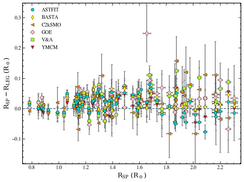
A&A proofs: manuscript no. article
Table 1. Set of fictitious stars to be characterised by SPInS. Here, inputs uniform truncated SFR (Eq. 6), and a uniform MDF, as priors.
to SPInS are log(L/L ), log(T eff ), and [M/H]. For all stars, we adopted For each star, the inferred age and mass are listed in Table 1. De-
a solar metallicity [M/H] = 0.00 ± 0.05 and the following uncertainties
σlog(L/L ) = 0.04 and σTeff = 100 K. The mass and age inferred by SPInS
pending on the position of a star in the H–R diagram, the solution
and their error bars are listed in Cols. 4 and 5. may be subject to an important degeneracy which is revealed in
the posterior probability distribution function (see the thorough
star log(L/L ) log(T eff ) A (Gyr) M/M discussions in, e.g. Jørgensen & Lindegren 2005; Takeda et al.
SF1 0.00 3.76 7.12 ± 3.72 0.96 ± 0.05 2007). We show in Fig. 3 several PDFs showing a different typi-
SF2 0.25 3.80 1.76 ± 1.30 1.16 ± 0.04 cal morphology which we examine below.
SF3 0.25 3.77 8.30 ± 2.20 1.02 ± 0.04
SF4 0.50 3.80 3.20 ± 0.85 1.23 ± 0.04 – Firstly, low-mass stars on the main sequence (hereafter MS)
SF5 0.50 3.75 7.54 ± 0.92 1.10 ± 0.04 lie in a region where the isochrones are crowded and thus can
SF6 0.50 3.70 9.34 ± 2.14 1.06 ± 0.06 be fitted by practically any isochrone. This is the case of star
SF7 0.83 3.80 2.49 ± 0.44 1.45 ± 0.06 SF1, close to the Sun, whose age is very ill-defined (see the
SF8 1.00 3.90 0.50 ± 0.18 1.70 ± 0.04 PDF in the left panel of top row in Fig. 3).
SF9 1.00 3.80 2.00 ± 0.24 1.59 ± 0.06 – Secondly, more massive stars, either on the MS or fully in-
SF10 1.00 3.70 4.80 ± 2.33 1.31 ± 0.15 stalled on the subgiant branch, have a rather well-defined age
SF11 1.50 4.00 0.15 ± 0.06 2.29 ± 0.05 and their PDF shows a single peak. This is the case for star
SF12 1.50 3.90 0.74 ± 0.04 2.12 ± 0.05 SF12 shown in the top row, right panel of Fig. 3, but also
SF13 1.50 3.70 1.82 ± 1.05 1.79 ± 0.27 for MS stars SF3, SF8, SF11, SF14, SF15, SF17, and sub-
SF14 2.00 4.10 0.04 ± 0.02 3.14 ± 0.06 giants SF5 and SF19. For stars close to the zero-age MS
SF15 2.00 4.00 0.33 ± 0.02 2.82 ± 0.06 such as star SF2, that is barely evolved stars, the one-peak
SF16 2.00 3.70 0.53 ± 0.10 2.77 ± 0.13 PDF (not shown) is very asymmetric. It is truncated close to
SF17 3.00 4.25 0.02 ± 0.01 5.63 ± 0.09 age ‘zero’ of the evolutionary tracks, meaning that for these
SF18 3.00 4.15 0.08 ± 0.00 4.97 ± 0.11 stars, tracks including the pre-main sequence phases should
SF19 3.00 3.90 0.11 ± 0.01 4.70 ± 0.13 be used. Moreover, since the region where star SF2 lies is
SF20 3.00 3.70 0.13 ± 0.01 4.63 ± 0.13 still crowded with isochrones, its PDF shows a very long tail
towards high ages up to about 8 Gyr.
– Thirdly, for stars of mass M & 1.2M which had a convective
3. Parameter inference for a set of fictitious stars core during the MS and are now lying in the so-called hook
region, in the vicinity of the end of the MS, several ages are
possible. However, these ages are not equally probable be-
cause of the different amounts of time spent either before
the red point of the evolutionary track (i.e. minimum of T eff
on the hook) or in the second contraction phase before the
blue point (i.e. maximum of T eff on the hook), or at the very
beginning of the subgiant phase. This translates into a PDF
generally showing two peaks, as can be seen in the bottom
row, left panel of Fig. 3 for star SF7, but the same behaviour
is seen for stars SF4, SF9, and SF18. For star SF20, located
close to the helium burning region where the star undergoes
blue loops, the PDF also shows two peaks, one of them being
very discreet.
– Fourthly, stars lying close to the red giant branch either show
a more or less well-defined peak in their PDF (such as stars
SF13 and SF16) or a flattened PDF (such as star SF6 shown
in the bottom row, right panel of Fig. 3 and star SF10).
Several indicators of a parameter, for instance the age, can be
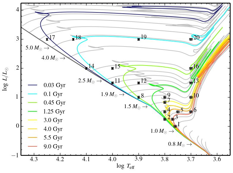
Fig. 2. Set of fictitious stars in the H–R diagram. Each star is labelled used. In Fig. 3, we show the median, the mean, and the posterior
by its number in Table 1. BaSTI stellar evolution tracks, some of which mode values given by SPInS for stars SF1, SF6, SF7, and SF12.
are labelled by their initial mass, are shown as well as isochrones, the The estimator of the mode is the maximum a posteriori (MAP).
ages of which are indicated in the legend starting from the youngest. However, in the case of star SF7, the age PDF is multimodal,
showing two maxima. Figure 3 shows that the mode provided
by SPInS is close to the second maximum when, intuitively, one
As a case study, corresponding to the most common demand would have taken the mode to be the value at the maximum of
for age and mass inference on a survey-wide scale, we first fo- the higher peak. It is because the mode, as calculated by SPInS,
cus on determining the properties of a small set of fictitious stars corresponds to the parameter set yielding the maximum posterior
with solar metallicity and spread across the H–R diagram. The probability given the observations (see Eq. 1) obtained in the
stars’ properties (luminosity, effective temperature, metallicity, grid’s parameter space (i.e. in the mass-age-metallicity space for
and their error bars) used as inputs to SPInS are listed and ex- this particular example). In contrast, the histogram showing the
plained in Table 1 and its caption. The positions of the stars in age PDF is obtained after an integration (i.e. marginalisation)
the H–R diagram are shown in Fig. 2. We used the solar-scaled with respect to mass and metallicity. For star SF7, the secondary
non-canonical BaSTI stellar model grid (cf. section 2.5), as well peak in the age histogram corresponds to a higher but narrower
as the IMF from Kroupa et al. (2013) given in Eqs. 3 and 5, a peak (especially in terms of the variables mass and metallicity)
Article number, page 6 of 16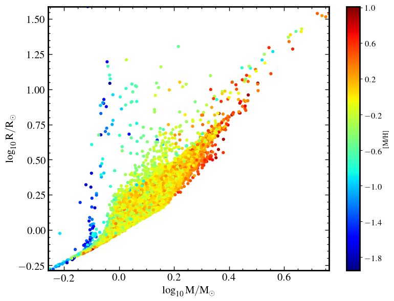
Y. Lebreton and D. R. Reese: SPInS, a pipeline for massive stellar parameter inference

Fig. 3. Morphology of the age posterior probability distribution function (PDF) for different positions (i.e. evolutionary states) in the H–R diagram.
The vertical lines indicate the values of the mean (blue continuous line), the mode (green dot-dashed line), and median (dashed red line). Top row,
left panel: ill-determined (star SF1). Top row, right panel: one single peak (star SF12). Bottom row, left panel: age degeneracy leading to two peaks
(star SF7). Bottom row, right panel: peculiar (star SF6). See discussion in the text.

in the original grid parameter space, thus explaining why it is             4. Parameter determination for stars in the
lower after marginalisation. On the other hand, the mass is well-              Geneva-Copenhagen Survey
determined for all stars, with PDFs mostly presenting one or two
peaks.                                                                      In this section, we aim at testing and validating the SPInS tool
                                                                            by characterising the stars of the Geneva-Copenhagen Survey
                                                                            (GCS). The GCS is a compilation of observational and stellar
                                                                            model-inferred properties of stars belonging to the solar neigh-
                                                                            bourhood. The first version of the GCS was presented and made
     In addition, SPInS provides triangle plots showing the distri-         public by Nordström et al. (2004, hereafter GCS04). It provides
butions of the fitted parameters and their correlations. Examples           a complete, magnitude-limited (V < 8.3), and kinematically un-
are shown in Fig. 4 for stars SF12 (top figure) and SF7 (bottom             biased sample of 16 682 nearby F and G dwarf stars. Many data
figure) where the distributions of age, mass, and metallicity are           can be found in the catalogue, of which the Hipparcos parallax,
shown. More complete triangle plots (not shown here) showing                metallicity, effective temperature, and Johnson V-magnitude are
other parameters (for instance the radius, surface gravity, seis-           of interest here. Later on, the data in the catalogue were assessed
mic indices, etc.) can be plotted according to the user’s choice.           and refined by Holmberg et al. (2007, 2009, hereafter GCS09).
SPInS also provides a number of files and figures making the                Then, Casagrande et al. (2011, hereafter GCS11) improved the
analysis of the intermediate and final results easy, including files        accuracy of the effective temperatures on the basis of the in-
listing the mean values of each estimated parameter, the median,            frared flux method, and consequently improved the metallicity
the one- and two-sigma percentiles, the correlations among pa-              scale. They also provided a proxy for the [α/Fe] ratio and red-
rameters, and the set of parameters corresponding to the mode.              dening E(B-V). Each version of the GCS also provides the age
                                                                                                                        Article number, page 7 of 16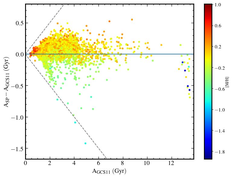
A&A proofs: manuscript no. article

                                                                                   – We used the following observational constraints for each
                                                                                     star: logarithm of effective temperature log T eff , absolute V-
                                                                                     magnitude in the Johnson band MV , and metallicity [M/H]
                                                                                     (not [Fe/H]).
                                                                                   – We took the same source for stellar models, that is the solar-
                                                                                     scaled canonical BaSTI grid described in Sect. 2.5 taken
                                                                                     from their website (Pietrinferni et al. 2004). However, the
                                                                                     grid used by Casagrande et al. (2011) was specially prepared
                                                                                     and is finer than the one available on the website. Further-
                                                                                     more, in contrast with Casagrande et al., we did not use the
                                                                                     isochrones but the evolutionary tracks, which are the direct
                                                                                     products of stellar evolution calculations.
                                                                                   – As was done in Casagrande et al. (2011), we adopted stellar
                                                                                     evolution models calculated for a solar-scaled mixture, but
                                                                                     we re-scaled the metallicity to mimic the α-element enrich-
                                                                                     ment. Since Casagrande et al. (2011) do not explicitly give
                                                                                     the re-scaling relation they adopted, we adopted the most
                                                                                     commonly used relation derived by Salaris et al. (1993)11 .
                                                                                     However, we checked that only minor differences are ob-
                                                                                     tained if the re-scaling of Nordström et al. (2004)12 , applied
                                                                                     in the GCS04, is used instead.
                                                                                   – To calculate the absolute magnitudes MV of each star, we
                                                                                     used the Johnson V-magnitude provided in the GCS09 and
                                                                                     the Hipparcos parallax provided in the GCS11 (i.e. the so-
                                                                                     called new Hipparcos reduction from van Leeuwen 2007).
                                                                                     We corrected the absolute magnitudes for the effects of ex-
                                                                                     tinction following Cardelli et al. (1989) with E(B-V) taken
                                                                                     from the GCS11.
                                                                                   – We assumed a Gaussian distribution in log T eff , MV , and
                                                                                     [M/H]. We, therefore, did not implement in SPInS the par-
                                                                                     ticular treatment of the magnitude distribution adopted by
                                                                                     Casagrande et al. (2011) to take into account the skewness of
                                                                                     the magnitude distribution that appears when the relative par-
                                                                                     allax error exceeds 10 per cent. Therefore, the present com-
                                                                                     parisons will not be valid for stars with high parallax errors.
                                                                                   – We adopted the same priors on the IMF, SFR, and MDF.
                                                                                     More precisely, we took the IMF from Salpeter (1955) as
                                                                                     given by Eqs. 2 and 4, a uniform truncated SFR (Eq. 6), and
                                                                                     the prescription of Casagrande et al. (2011) for the particular
                                                                                     MDF of the stars in the GCS11 (see their Appendix A).

                                                                              4.1. Ages
                                                                              We present in Fig. 5 the age residuals between the ages obtained
                                                                              by SPInS (mean ages) and those of the GCS11 (referred to as
                                                                              ‘expected’ age in their terminology but which also corresponds
Fig. 4. Triangle plots with the distributions of fitted parameters includ-    to the mean value). The ages of 14 757 stars out of 16 682 could
ing 2D correlations among parameters for a number of MCMC walkers.            be determined. For the remaining stars, either the parallax, effec-
Mean values are indicated by blue continuous lines. The point density         tive temperature, or metallicity were unavailable. In Fig. 5 (left
is indicated by the greyscale of the distributions, with the darker, denser   panel), we only retained the stars for which the age-dating is con-
regions towards the maximum of the PDF. The contour lines indicate            sidered to be of good quality under the criteria of Casagrande
0.5, 1.0, 1.5, and 2.0 sigma departures from the maximum. The top             et al. (2011), that is the relative error on age is lower than 25
figure shows the results for star SF12, whereas the bottom figure corre-      per cent and the absolute age error is lower than 1 Gyr. This
sponds to star SF7.                                                           represents a total of 5040 stars. The comparison is very satisfac-
                                                                              tory since the differences in ages between SPInS and the GCS11
                                                                              mostly remain lower than 25 per cent. In Fig. 5 (right panel), we
                                                                              considered all stars with a determined age and a parallax error
and mass of the stars, and related uncertainties, derived by means            lower than 10 per cent (to minimise the possibility of a skew-
of a Bayesian analysis.                                                       ness in the V-magnitude distribution, see the discussion in Sect.
                                                                              4 above). Even if the differences between the SPInS and GCS11
    In order to compare the results of SPInS with those of
Casagrande et al. (2011), we used SPInS to determine the ages                 11
                                                                                 In Salaris et al. (1993), the solar-scaled Z is re-scaled as Zα according
and masses of stars in the GCS. We adopted, as far as possible,               to Zα = Z × (0.638 × 10[α/Fe] + 0.362)
the assumptions made by these authors, namely:                                12
                                                                                 [M/H]α = [M/H] + 0.75 × [α/Fe]

Article number, page 8 of 16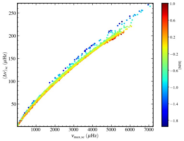
Y. Lebreton and D. R. Reese: SPInS, a pipeline for massive stellar parameter inference

Fig. 5. Age residuals (ASP − AGCS11 ) between the mean age value delivered by SPInS (ASP ) and the expected (i.e. also mean) age (AGCS11 ) given in
the GCS11 (Casagrande et al. 2011). The horizontal grey line shows the locus of equal ages and the dashed lines are for ages differing by ±25 per
cent. The colours distinguish stars according to their metallicity. Left figure: 5040 stars with good ages as defined by Casagrande et al. (see text),
with no filtering of the parallax error. Right figure: 10 865 stars with determined ages, all stars having a parallax error lower than 10 per cent.

ages are larger in that case, there are only 503 stars out of 10 865        masses of 14 757 out of 16 682 could be determined. In the fig-
(that is less than 5 per cent) showing an age difference larger             ure, we only retained stars for which we consider the mass to be
than 25 per cent.                                                           of good quality, that is the relative error on mass is lower than 10
                                                                            per cent. This represents a total of 12 704 stars. The comparison
                                                                            is very satisfactory since the differences in mass between SPInS
4.2. Masses                                                                 and GCS11 values mostly remain lower than 10 per cent. The
                                                                            disparity of SPInS and GCS11 results is less important for the
                                                                            masses than for the ages because, for a given set of stellar evolu-
                                                                            tionary tracks, the mass degeneracy in the Hertzsprung-Russell
                                                                            diagram is less marked than the degeneracy affecting the ages, in
                                                                            particular at the end of the main sequence.

                                                                            4.3. Radii, surface gravities, and mean seismic parameters
                                                                            In addition to the ages and masses of the stars in the GCS11,
                                                                            SPInS provided several interesting stellar properties related to
                                                                            stellar evolutionary tracks or that can easily be derived from
                                                                            them. In particular, we show in Fig. 7 the Kiel diagram (log T eff −
                                                                            log g), the mass-radius relation, and the asteroseismic diagram
                                                                            (νmax,sc –h∆νisc ) based on seismic indices. The discussion of the
                                                                            results is beyond the scope of this paper, although some well-
                                                                            known trends can be highlighted, in particular the position of
                                                                            stars as a function of their metallicity in the Kiel diagram result-
                                                                            ing from their different internal structures. It is worth pointing
                                                                            out that the combination of such diagrams, involving large stel-
                                                                            lar samples, can be very valuable when used in studies of Galac-
Fig. 6. Mass residuals (MSP − MGCS11 ) between the mean mass value
(MSP ) delivered by SPInS and the expected (i.e. also mean) mass            tic Archaeology (Miglio et al. 2009, 2013) thus making SPInS a
(MGCS11 ) given in the GCS11 (Casagrande et al. 2011) for the 12 704        very interesting tool in this respect.
stars with good masses as defined in the text, with no filtering on the
parallax error. For ten stars, the masses determined by SPInS and by
Casagrande et al. differ by more than 10 per cent. The horizontal grey      5. Further applications of SPInS for single stars
line shows the locus of equal masses and the dashed lines are for masses
                                                                            5.1. Stars observed in interferometry
differing by ±10 per cent. The colours distinguish stars according to
their metallicity.                                                          With interferometry, the angular diameters of stars can be mea-
                                                                            sured which in turn gives a direct access to their radii, pro-
                                                                            vided their distance is known. These measurements are there-
   In Fig. 6, we show the mass residuals between the masses                 fore independent of stellar models (except for limb-darkening
(mean values) derived by SPInS and those in the GCS11 (ex-                  of the stellar disc which has to be corrected for, based on stel-
pected values corresponding to mean ones). As for the ages, the             lar model atmospheres). Ligi et al. (2016) obtained the radii of
                                                                                                                        Article number, page 9 of 16
A&A proofs: manuscript no. article
Fig. 7. Stellar parameters inferred with SPInS for about 14 750 stars in the GCS11 catalogue. Left figure: Kiel diagram. Central figure: Mass-Radius
relation. Right figure: Asteroseismic νmax,sc –h∆νisc diagram.
18 stars (eleven of them being exoplanet hosts) from interfer- However, when individual frequencies cannot be extracted from
ometry, together with their bolometric fluxes from photometry the pressure-mode oscillation spectrum, SPInS can give some
which allowed them to infer the effective temperatures. Starting characteristics of a star provided the seismic indices νmax,obs or
from these data, metallicities taken in the literature, and model h∆νiobs , or both have been estimated from observations. Indeed,
isochrones, they applied a Bayesian method with flat priors to SPInS can take νmax,obs and h∆νiobs as input constraints which,
infer the mass and age of each star. through the scaling relations (Eqs. 11 and 12), provides hints on
By using Ligi et al.’s radii, effective temperatures, and metal- the stellar mass and radius, provided the effective temperature is
licities as input constraints for SPInS, we inferred the masses and known. In the following, we study two stellar samples (an artifi-
ages of the stars. We used the solar-scaled non-canonical BaSTI cial and a real one), for which SPInS inferences of mass, radius,
grid including convective core overshooting and we assumed flat and age based on νmax,obs and h∆νiobs can be compared with the
priors on mass and metallicity, but a uniform truncated prior on results of careful inferences based on individual oscillation fre-
age (Eq. 6). In Fig. 8, we compare SPInS masses and ages with quencies.
the values from Ligi et al. (2016). Overall, the comparison is
satisfactory, except for one star, HD 167042. If we exclude this
5.2.1. Artificial stars: Reese et al. (2016)’s hare and hounds
star, the mean mass (respectively age) difference is of 4 (respec-
sample
tively 19) per cent and maximum differences are of 15 (respec-
tively 84) per cent. For HD 167042, shown with pink diamonds As a first case study, we consider ten artificial stars, built and
in Fig. 8, SPInS’s mass is much smaller than the one found by studied in the hare-and-hounds exercise of Reese et al. (2016).
Ligi et al. (2016) while SPInS’s age is much larger. Understand- To build each star, a stellar model was calculated for a given
ing the origin of the difference is beyond the scope of this paper. mass and age. Then, starting from this model, a hare group sim-
However, Ligi et al. pointed out that, for this star, their results ulated observational quantities of an artificial star, that is its os-
are not consistent with the models. Moreover, we point out that cillation frequencies and classical parameters. Finally, the results
it may currently be difficult to characterise this K1IV subgiant. were communicated to several hound teams who applied distinct
Indeed, doubts remain about its effective temperature which is optimisation methods to characterise the stars on the basis of
found to be 4547 ± 49 K when combining interferometry and these constraints. We list the properties of the ten stars in Ta-
photometry (Ligi et al. 2016) and 4983 ± 10 K when using high ble 2. Their positions in the H–R diagram are shown in Fig. 1 of
resolution spectroscopy (Maldonado & Villaver 2016). Reese et al. (2016).
In the future, large samples of stars with angular radii We applied SPInS to these stars taking their ‘observed’14 lu-
measured by interferometry will be available. In particular, minosity, effective temperature, metallicity, νmax,obs , and h∆νiobs
the CHARA/SPICA project13 , based on the new visible inter- as input constraints. We used the solar-scaled non-canonical
ferometric instrument CHARA/SPICA currently under design BaSTI grid including convective core overshooting and we took
(Mourard et al. 2018), aims at constituting a homogeneous cat- flat priors on mass, age, and metallicity. In Fig.9, we show how
alogue of about a thousand angular diameters of stars spanning the masses and radii inferred both by SPInS and by the teams that
the whole H–R diagram, including hosts of exoplanetary sys- participated in the exercise of Reese et al. (2016) reproduce the
tems and stars observable in asteroseismology. SPInS will enable true properties of the –artificial– stars. With SPInS, mean differ-
a rapid characterisation of the fundamental parameters of these ences with the artificial stars are of 2.8 per cent on the predicted
stars (mass, age), thus opening the way to an in-depth analysis mass and of 1.1 per cent on the radius. The maximum differences
of their internal structure, planet characterisation, etc. are for Blofeld and to a lesser extent Diva. For Blofeld, the differ-
ence is of about 11 per cent on mass and of 3.7 per cent on radius.
5.2. Solar-like oscillators It is worth noting that both of these simulated stars have the same
mass (Mobs = 1.22M ) and are both on the subgiant branch but
SPInS has not been designed for the purpose of delivering a have different chemical compositions. Moreover, the BaSTI grid
precise asteroseismic diagnosis. To perform detailed asteroseis- models (Pietrinferni et al. 2004) have not been calculated with
mic analysis, one can use, for instance, the public AIMS tool the same input physics and parameters as Reese et al. (2016)’s
described in Lund & Reese (2018) and Rendle et al. (2019).
14
Here, ‘observed’ values correspond to simulated results including a
13
https://lagrange.oca.eu/fr/spica-project-overview realistic error realisation.
Article number, page 10 of 16Y. Lebreton and D. R. Reese: SPInS, a pipeline for massive stellar parameter inference
Table 2. Simulated properties for the set of artificial stars of Reese et al. (2016). These properties are taken from their Table 1 except for h∆νiobs that
we calculated as the least-square mean of the individual frequencies of radial modes given in Table A.1 of Reese et al. (‘obs’ therefore corresponds
to simulated results including a realistic error realisation). The ‘true’ masses, radii, and ages (i.e. from the original stellar models) are provided in
the last three columns.
star Lobs T eff,obs [M/H]obs νmax,obs h∆νiobs M R A
(L ) (K) (µHz) (µHz) (M ) (R ) (Gyr)
Aardvark 0.87 ± 0.03 5720 ± 85 +0.02 ± 0.09 3503 ± 165 144.47 ± 0.01 1.00 0.959 3.058
Blofeld 2.02 ± 0.06 5808 ± 85 +0.04 ± 0.09 1750 ± 100 94.14 ± 0.01 1.22 1.359 2.595
Coco 0.73 ± 0.02 5828 ± 85 −0.74 ± 0.09 3634 ± 179 162.14 ± 0.02 0.78 0.815 9.616
Diva 2.14 ± 0.06 5893 ± 85 +0.03 ± 0.09 2059 ± 101 95.77 ± 0.01 1.22 1.353 4.622
Elvis 1.22 ± 0.04 5900 ± 85 +0.04 ± 0.09 2493 ± 127 119.96 ± 0.01 1.00 1.087 6.841
Felix 4.13 ± 0.12 6175 ± 85 +0.06 ± 0.09 1290 ± 66 69.39 ± 0.02 1.33 1.719 2.921
George 4.31 ± 0.13 6253 ± 85 −0.03 ± 0.09 1311 ± 67 70.25 ± 0.04 1.33 1.697 2.944
Henry 1.94 ± 0.06 6350 ± 85 −0.35 ± 0.09 2510 ± 124 116.46 ± 0.04 1.10 1.138 2.055
Izzy 2.01 ± 0.06 6431 ± 85 −0.34 ± 0.09 2319 ± 124 115.85 ± 0.03 1.10 1.141 2.113
Jam 3.65 ± 0.11 6503 ± 85 +0.09 ± 0.09 1758 ± 89 86.54 ± 0.06 1.33 1.468 1.681
models. Indeed, Reese et al.’s models of Diva and Blofeld were 5.2.2. Real stars: the Kepler LEGACY sample
calculated with different amounts of convective core overshoot-
ing. Moreover, Blofeld includes atomic diffusion, a different so- In the same vein, we now consider 66 stars belonging to the
lar mixture, and a truncated atmosphere. We also note that Diva Kepler seismic LEGACY sample (e.g. Lund et al. 2017). Each
is one of the least well-fitted stars in Reese et al. (2016). star has at least 12 months of Kepler short-cadence data. There-
fore, these stars are among the solar-like oscillators observed by
Kepler that have the highest signal-to-noise ratios. As a conse-
Overall, as can be seen in Fig.9, except for the cases of quence, their individual oscillation frequencies inferred by Lund
Blofeld and Diva that, in all likelihood result from identified dif- et al. (2017) are among the most precise to-date for solar-like
ferences in stellar models, the masses and radii inferred by SPInS pulsators while their effective temperatures and metallicity are
compare very well with those inferred from a thorough astero- also available. Silva Aguirre et al. (2017) performed a thorough
seismic diagnosis based on individual oscillations frequencies. modelling of the stars, with different optimisation methods im-
This confirms the power of the scaling relations to quite reason- plemented in six pipelines. All pipelines took into account the
ably infer the mass and radius of solar-like oscillators (Chaplin complete set of oscillation frequencies, either individual fre-
et al. 2014). quencies or frequency separation ratios, or a combination thereof
(see Silva Aguirre et al. 2017, for details).
We have analysed these stars with SPInS in a simplified way,
As for the age, we show in Fig. 9 that the situation is not as
by considering as observational constraints T eff , [Fe/H], log g,
good. Indeed, the scaling relations do not constrain this param-
h∆νi, and νmax . We used the solar-scaled non-canonical BaSTI
eter tightly and the age inference is highly sensitive to the input
grid including convective core overshooting. As for the priors,
physics of stellar models (see e.g. Lebreton et al. 2014). With
we adopted the two-slopes IMF from Eq. 3 with Kroupa et al.
SPInS, we find a mean difference of 28 per cent on age for the
(2013)’s coefficients (Eq. 5), a uniform truncated SFR (Eq. 6),
ten stars while the mean difference obtained with the pipelines in
and a flat prior on the MDF. We then compared SPInS inferences
Reese et al. (2016) is of 23 per cent. We get a maximum differ-
with those reported in Silva Aguirre et al. (2017).
ence on age of 143 per cent for Blofeld. Even if, in this particular
study, the ages are very well recovered by SPInS for seven artifi- In the left panel of Fig. 10, we show the residuals (RSP −RLEG )
cial stars out of ten, real stars by far host much more subtle phys- between the radius of each star inferred by SPInS (RSP ) and the
ical processes than stellar models are able to describe. Therefore, values RLEG obtained from full optimisations as reported in Silva
individual oscillation frequencies if available, or some combina- Aguirre et al. (2017). In the right panel of Fig. 10, we show the
tions thereof, should always be preferred to the seismic indices residuals (MSP − MLEG ) between the masses. If we exclude the
when a precise and accurate age estimate is being sought (see for result of the GOE pipeline for star KIC 7771282 (shown by
instance the study of the CoRoT target HD 52265 by Lebreton pink diamonds at RSP ≈ 1.66R , RLEG,GOE ≈ 1.4R and at
& Goupil 2014). MSP ≈ 1.3M , MLEG,GOE ≈ 0.8M in the panels of Fig. 10),
which is well outside the range found by the others, maximum
differences on the radius between SPInS and the six pipelines,
We also would like to point out that the scaling relations are over 66 stars, range from 3.5 to 9 per cent, while mean differ-
much less efficient at predicting masses, radii, and ages when the ences are in the range of 1.3-2.5 per cent. As for the mass, max-
luminosities of the stars are not known. This was checked by ap- imum differences are in the range of 16-26 per cent, while mean
plying SPInS to the ten stars using only T eff , [Fe/H], νmax,obs , and differences are in the range of 5-6.5 per cent. Finally, for the
h∆νiobs as input constraints and removing the constraint on lu- ages, we find larger mean differences ranging from 25 to 32 per
minosity. In that case, the mean errors on the predicted masses, cent. To get a clearer picture, if we consider the objectives of
radii, and ages are higher, with values of 6, 2, and 64 per cent the PLATO mission (Rauer et al. 2014), that is to reach uncer-
respectively and maximum errors of 19, 7 and 300 per cent for tainties of less than 2 per cent on the radius, 10 per cent on the
Blofeld. This favours combining all possible classical and as- mass, and 10 per cent on the age of an exoplanet host-star to be
teroseismic parameters to characterise stars, and reinforces the able to characterise its exoplanet correctly, there are three stars
need for precise luminosities from the Gaia mission and radii for which SPInS’s radius is outside the interval corresponding to
from interferometry or eclipsing binary light curves. the extreme values provided by the six pipelines by more than
Article number, page 11 of 16You can also read