Updated Binary Pulsar Constraints on Einstein-aether Theory in Light of Gravitational Wave Constraints on the Speed of Gravity
←
→
Page content transcription
If your browser does not render page correctly, please read the page content below
Updated Binary Pulsar Constraints on Einstein-æther
                                        Theory in Light of Gravitational Wave Constraints on
                                        the Speed of Gravity
arXiv:2104.04596v1 [gr-qc] 9 Apr 2021

                                                     Toral Gupta1 , Mario Herrero-Valea2,3 , Diego Blas4 , Enrico
                                                     Barausse2,3 , Neil Cornish1 , Kent Yagi5 and Nicolás Yunes6
                                                     1
                                                      eXtreme Gravity Institute, Department of Physics, Montana State University,
                                                     Bozeman, Montana 59717, USA.
                                                     2
                                                         SISSA, Via Bonomea 265, 34136 Trieste, Italy & INFN, Sezione di Trieste.
                                                     3
                                                      IFPU - Institute for Fundamental Physics of the Universe,
                                                     Via Beirut 2, 34014 Trieste, Italy.
                                                     4
                                                      Theoretical Particle Physics and Cosmology Group, Department of Physics, King’s
                                                     College London, Strand, London WC2R 2LS, UK.
                                                     5
                                                         Department of Physics, University of Virginia, Charlottesville, Virginia 22904, USA.
                                                     6
                                                      Illinois Center for Advanced Studies of the Universe, Department of Physics,
                                                     University of Illinois at Urbana-Champaign, Urbana, Illinois, 61820 USA.

                                                     E-mail: toral.gupta@montana.edu

                                                     Abstract. Timing of millisecond pulsars has long been used as an exquisitely precise
                                                     tool for testing the building blocks of general relativity, including the strong equivalence
                                                     principle and Lorentz symmetry. Observations of binary systems involving at least one
                                                     millisecond pulsar have been used to place bounds on the parameters of Einstein-
                                                     æther theory, a gravitational theory that violates Lorentz symmetry at low energies
                                                     via a preferred and dynamical time threading of the spacetime manifold. However,
                                                     these studies did not cover the region of parameter space that is still viable after the
                                                     recent bounds on the speed of gravitational waves from GW170817/GRB170817A. The
                                                     restricted coverage was due to limitations in the methods used to compute the pulsar
                                                     “sensitivities”, which parameterize violations of the strong-equivalence principle in these
                                                     systems. We extend here the calculation of pulsar sensitivities to the parameter space
                                                     of Einstein-æther theory that remains viable after GW170817/GRB170817A. We show
                                                     that observations of the damping of the period of quasi-circular binary pulsars and of
                                                     the triple system PSR J0337+1715 further constrain the viable parameter space by
                                                     about an order of magnitude over previous constraints.

                                                     PACS numbers: 04.30Db,04.50Kd,04.25Nx,97.60Jd

                                        Submitted to: Class. Quantum Grav.
Updated Binary Pulsar Constraints on Einstein-æther theory                              2

1. Introduction

Lorentz symmetry has been the foundation of the magnificent edifice of theoretical
physics for more than a century, playing a central role in special and general relativity
(GR), as well as in the quantum theory of fields. Because of its special status,
Lorentz invariance has been tested to exquisite precision in the matter sector via
particle physics experiments [48, 49, 53, 44]. More recently, this experimental program
has been extended to the matter-gravity [47], dark matter [16, 13], and pure-gravity
sectors [41, 52], where bounds on Lorentz violations (LVs) have been historically looser
(because of the intrinsic weakness of the gravitational interaction).

Compelling theoretical reasons to seriously consider the possibility of LVs in the purely
gravitational sector were provided by the realization that they could generate a better
behavior in the ultraviolet (UV) limit. In particular, P. Hořava [38] showed that
by allowing for a non-isotropic scaling between space and time, one can construct
a theory that is power-counting renormalizable in the UV. Renormalizability beyond
power counting (i.e. pertubative renormalizability) in special (“projectable”) versions of
Hořava gravity has also been proven [10].

The low-energy limit of Hořava gravity reduces to “khronometric theory” [15, 42], which
consists of GR plus an additional hypersurface-orthogonal and timelike vector field,
often referred to as the “æther”. Because this vector field is hypersurface orthogonal,
it selects a preferred spacetime foliation, which makes LVs manifest. A more general
boost-violating low-energy gravitational theory, however, can be obtained by relaxing
the assumption that the æther be hypersurface-orthogonal, in which case it selects a
preferred time threading of the spacetime rather than a preferred foliation. The resulting
theory is known as Einstein-æther theory [45].

Despite allowing for an improved UV behavior, LVs in gravity face long-standing
experimental challenges, particularly when it comes to their percolation into the matter
sector, where particle physics experiments are in excellent agreement with Lorentz
symmetry. While some degree of percolation is inevitable, because of the coupling
between matter and gravity, mechanisms suppressing it have been put forward, including
suppression by a large energy scale [57], or the effective emergence of Lorentz symmetry
at low energies as a result of renormalization group flows [23, 12, 11] or accidental
symmetries [37].

At the same time, purely gravitational bounds on LVs are becoming increasingly
compelling.   The parameters (“coupling constants”) of both Einstein-æther and
khronometric theory have been historically constrained by theoretical considerations
(absence of ghosts and gradient instabilities [18, 40, 36], well-posedness of the
Cauchy problem [59]), by the absence of vacuum Cherenkov cascades in cosmic-
ray experiments [29]), by solar-system tests [66, 33, 18, 19, 54], by observations of
Updated Binary Pulsar Constraints on Einstein-æther theory                               3

the primordial abundances of elements from Big-Bang nucleosynthesis [22], by other
cosmological tests [8], and by precision timing of binary pulsars (where LVs generically
predict violations of the strong equivalence principle) [32, 31, 70, 71, 9]. More recently,
the coincident detection [3, 2] of gravitational waves (GW170817) and gamma rays
(GRB170817A) emitted by the coalescence of two neutron stars and the subsequent
kilonova explosion has allowed extremely strong constraints on the propagation speed
of gravitational waves, which must equal that of light to within‡ 10−15 [1], which in turn
places even more stringent bounds on the couplings of both theories [30, 58, 59, 55].

The bounds from the coincident GW170817/GRB170817A observations force us to
rethink the parameter spaces of both Einstein-æther and khronometric theory, as the
only currently allowed regions appear to be ones that were previously thought to be
of little interest, and which were not explored extensively. In the case of khronometric
theory, Refs. [58, 9] found that the couplings that remain viable after GW170817 and
GRB170817 produce exactly no deviations away from the predictions of GR, not only
in the solar system, but also in binary systems of compact objects, be they black holes
(BHs) or neutron stars (NSs), to leading post-Newtonian (PN) order. Reference [34]
extended this result to the quasinormal modes of spherically symmetric black holes and
to fully non-linear (spherical) gravitational collapse, where again no deviations from
the GR predictions are found. It would therefore seem that the most promising avenue
to further test khronometric theory may be provided by cosmological observables (e.g.
Big-Bang nucleosynthesis abundances or CMB physics), where the viable couplings do
produce non-vanishing deviations away from the GR phenomenology.

Like for khronometric theory, the parameter space where detailed predictions for
isolated/binary pulsars were obtained in Einstein-æther theory [70, 71] does not include
the region singled out by the combination of the GW170817/GRB170817A bound and
existing solar-system constraints (see Ref. [59] for a discussion). The goal of this paper
is therefore to extend the previous analysis of binary/isolated-pulsar data by some of
us [70, 71] to this region of parameter space. This will require a significant modification
of the formalism that Refs. [70, 71] utilized to calculate pulsar “sensitivities”, i.e. the
parameters that quantify violations of the strong-equivalence principle in these systems.
Moreover, we will extend our analysis to include additional data over that considered
in Refs. [70, 71], namely the triple system PSR J0337+1715 [7]. Overall, we find that
observations of the damping of the period of quasi-circular binary pulsars, and that of
the triple system PSR J0337+1715, reduce the viable parameter space of Einstein-æther
theory by about an order of magnitude over previous constraints.

We will also amend an error (originally pointed out in Ref. [67]) in the calculation of
the strong-field preferred-frame parameters α̂1 and α̂2 for isolated pulsars, which were
presented in Refs. [70, 71]. While we have checked that this error does not impact the
bounds presented in Refs. [70, 71], we present in Appendix A a detailed derivation of
‡ See also [24] for looser bounds coming from mergers of black holes.
Updated Binary Pulsar Constraints on Einstein-æther theory                                                 4

α̂1 and α̂2 for possible future applications, also correcting a few typos present in the
original calculation of Ref. [67].

This paper is organized as follows. In Sec. 2 we give a succinct introduction to Einstein–
æther theory, including the modified field equations and the current observational
bounds on the coupling constants. In Sec. 3 we introduce the concept of stellar
sensitivities as parameters regulating violations of the strong equivalence principle.
Solutions describing slowly moving stars are derived in Sec. 4, and they are used in Sec. 5
to compute the sensitivities. Section 6 uses the sensitivities to obtain the constraints on
Einstein–æther theory resulting from observations of binary and triple pulsar systems.
We summarize our conclusions in Sec. 7. Appendix A contains a calculation of the
strong-field preferred-frame parameters α̂1 and α̂2 in Einstein-æther theory, fixing an
oversight in [70], which was pointed out by [67], and correcting also a few typos present
in [67] itself. We will adopt units where c = 1 and a signature + − −−, in accordance
with most of the literature on Einstein-æther theory.

2. Einstein æther theory

In order to break boost (and thus Lorentz) symmetry, Einstein-æther theory introduces
a dynamical threading of the spacetime by a unit-norm, time-like vector field U . This
vector field, often referred to as the æther, physically represents a preferred “time
direction” at each spacetime event. Requiring the action to also include the usual
spin-2 graviton of GR, to be quadratic in the æther derivatives, and to feature no direct
coupling between the matter and the æther (so as to enforce the weak equivalence
principle, i.e. the universality of free fall, and the absence of matter LVs at tree level),
one obtains the action [45, 43]
                            Z h
                        1             1
               S=−              R + cθ θ2 + cσ σµν σ µν + cω ωµν ω µν + ca Aµ Aµ
                     16πG             3
                                 i√
                 + λ(U Uµ − 1) −g d4 x + Smat (ψ, gµν ),
                       µ
                                                                                        (1)

where R is the four-dimensional Ricci scalar, g the determinant of the metric, G
the bare gravitational constant (related to the value GN measured locally by GN =
G/(1 − ca /2) [22, 41]), ψ collectively denotes the matter degrees of freedom, λ is a
Lagrange multiplier enforcing the æther’s unit norm, cθ , cσ , cω and ca are dimensionless
constants§, and we have decomposed the æther congruence into the expansion θ, the
§ Note that much of the earlier literature on Einstein-æther theory uses a different set of coupling
constants ci (i = 1, . . . , 4), which are related to our parameters by c1 = (cω + cσ )/2, c2 = (cθ − cσ )/3,
c3 = (cσ − cω )/2 and c4 = ca − (cσ + cω )/2.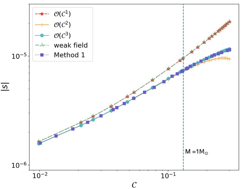
Updated Binary Pulsar Constraints on Einstein-æther theory                                      5

shear σµν , the vorticity ωµν and the acceleration Aµ as follows:
                                        Aµ = U ν ∇ν U µ ,                                     (2)
                                                    µ
                                          θ = ∇µ U ,                                          (3)
                                                       1
                              σµν = ∇(ν Uµ) + A(µ Uν) − θhµν ,                                (4)
                                                       3
                                  ωµν = ∇[ν Uµ] + A[µ Uν] ,                                   (5)
with hµν = gµν − Uµ Uν the projector onto the hyperspace orthogonal to U .

By varying the action with respect to the metric, the æther and the Lagrange multiplier,
and by eliminating the latter from the equations, one obtains the generalized Einstein
equations
                                           Æ          mat
                           Eαβ ≡ Gαβ − Tαβ   − 8πGTαβ     =0                        (6)
and the æther equations

                                αν          cσ + cω       ν α
                 Ƶ = ∇α J − ca −                     Aα ∇ U hµν = 0,                    (7)
                                               2
where Gαβ is the Einstein tensor, the æther stress-energy tensor is
                                            cω + cσ
  Æ
Tαβ = ∇µ J(α µ Uβ) − J µ (α Uβ) − J(αβ) U µ +         [(∇µ Uα )(∇µ Uβ ) − (∇α Uµ )(∇β U µ )]
                                                2
              µν                   cσ + cω  2                  1
    + Uν (∇µ J )Uα Uβ − ca −                  A Uα Uβ − Aα Aβ + M σρ µν ∇σ U µ ∇ρ U ν gαβ ,
                                      2                           2
                                                                                         (8)
with
   J α µ ≡ M αβ µν ∇β U ν ,

      αβ        cσ + cω      αβ       cθ − cσ    α β      cσ − cω
   M µν =                   h gµν +             δµ δν +             δνα δµβ + ca U α U β gµν ,
                    2                    3                   2
and the matter stress-energy tensor is defined as usual by
                                    αβ        2 δSmat
                                  Tmat  ≡ −√            .                                      (9)
                                               −g δgαβ

As already mentioned, a number of experimental and theoretical results constrain
Einstein-æther theory and the couplings ci . In more detail, perturbing the field equations
about Minkowski space yields propagation equations for spin-0 (i.e. scalar), spin-1 (i.e.
vector) and spin-2 (i.e. tensor gravitons). Their propagation speeds are respectively
given by [40]
                                                 1
                                      c2T =          ,                                 (10)
                                             1 − cσ
                                         cσ + cω − cσ cω
                                 c2V =                   ,                             (11)
                                           2ca (1 − cσ )
                                     (cθ + 2cσ )(1 − ca /2)
                             c2S =                           .                         (12)
                                    3ca (1 − cσ )(1 + cθ /2)
Updated Binary Pulsar Constraints on Einstein-æther theory                                6

In order to ensure stability at the classical level (i.e. no gradient instabilities) and at
the quantum level (i.e. no ghosts) one needs to have c2T > 0, c2V > 0 and c2S > 0 [40, 36].
Furthermore, significantly subluminal graviton propagation would cause ultrarelativistic
matter to lose energy to gravitons via a Cherenkov-like process [29]. Since this effect
is not observed e.g. in ultrahigh energy cosmic rays, one must have c2I & 1 − O(10−15 )
(with I = T, V, S). More recently, the coincident detection of a neutron-star merger in
GW170817 (gravitational waves) and GRB170817A (gamma rays) had led to the bound
−3 × 10⁻¹⁵ < cT − 1 < 7 × 10⁻¹⁶ [1].

Expanding the field equations through 1PN order leads to the conclusion that
the 1PN dynamics is well described (like in GR) by the parametrized PN (PPN)
expansion [66, 54]. However, unlike in GR, the preferred frame parameters α1 and
α2 appearing in the PPN expansion do not vanish, but are given by [33]
                                    cω (ca − 2cσ ) + ca cσ
                               α1 = 4                      ,                           (13)
                                      cω (cσ − 1) − cσ
                                  α1 3(ca − 2cσ )(cθ + ca )
                             α2 =   +                        .                         (14)
                                  2     (2 − ca )(cθ + 2cσ )

Solar system experiments require |α1 | . 10−4 and |α2 | . 10−7 [66, 54]. By saturating
these bounds (i.e. requiring in particular that |α1 | . 10−4 but not |α1 |  10−4 ) and
combining with the constraints on the propagation speeds, one finds cσ ≈ O(10−15 ),
ca ≈ O(10−4 ), and cθ ≈ 3ca [1+O(10−3 )]. The resulting experimentally viable parameter
space, therefore, is effectively (i.e. to within a fractional width of 10−4 or better in the
parameters) one-dimensional: cσ , ca , cθ ≈ 0, but cω is essentially unconstrained [59].

Another viable region of the parameter space can be obtained by not saturating the
PPN constraints [59]. In more detail, one may require |α1 | be much smaller than its
upper limit, so as to automatically satisfy the bound on α2 (since α2 ∝ α1 if cσ ≈ 0,
as imposed by GW170817 and GRB170817A). This leads to |ca | . 10−7 and thus to an
effectively two-dimensional experimentally viable parameter space (cθ , cω ), with the only
additional requirement that |cθ | . 0.3 to ensure that the production of light elements
during Big Bang Nucleosynthesis gives predictions in agreement with observations [22].

Both of the viable regions of parameter space identified above were not considered
in Refs. [70, 71], where neutron-star sensitivities in Einstein-æther theory were first
computed. This is because back when Refs. [70, 71] were written, the strongest
constraints available were the solar system ones (since the GW170817/GRB170817A
constraint was not yet available). Therefore, Refs. [70, 71] solved for ca and cθ in
terms of cσ , cω , α1 and α2 , and varied the latter two within the solar system bounds
|α1 | . 10−4 and |α2 | . 10−7 . Since these bounds are narrow, this restricted the
exploration of the parameter space to a region very close to α1 ∼ 0 ∼ α2 , which
in turn implies that ca ∼ −cθ ∼ 2cω cσ /(cσ + cω ). This selects a two-dimensional
hypersurface in the (cθ , cσ , cω , ca ) parameter space. If after this selection, one were
Updated Binary Pulsar Constraints on Einstein-æther theory                                  7

to impose the GW170817/GRB170817A constraint (i.e. |cσ | . 10−15 ), one would then
find that |ca | . 10−15 and |cθ | . 10−15 , leaving only cω free. However, because of the
Cherenkov bound [29], one must have 0 ≤ cω . cσ /[3(1 − cσ )] [41], and cω is therefore
constrained to the small region 0 ≤ cω . 10−15 . In contrast, the first region listed above
[(cθ , cσ , ca ) . 10−4 with cω kept free] is much larger, precisely because we are now not
restricting ourselves to a two-dimensional hypersurface of parameter space.

3. Strong-equivalence principle violations and sensitivities

Most theories extending/modifying GR involve additional degrees of freedom besides
the massless tensor graviton of GR. These additional gravitational polarizations cannot
directly couple with matter significantly, to avoid introducing unwanted fifth forces
in particle physics experiments, and to prevent violations of the weak equivalence
principle (and particularly violations of the universality of free fall for weakly gravitating
objects). Nevertheless, effective couplings between the extra gravitons and matter may
be mediated by the metric perturbations (i.e. by the tensor gravitons present also in
GR), which are typically coupled non-minimally to the extra gravitational degrees of
freedom. These effective couplings become important when the metric perturbations
are “large”, which is the case for strongly gravitating systems such as those involving
NSs and/or BHs.

A useful way to parametrize this effective coupling is provided by the sensitivity
parameters. Because of the aforementioned effective couplings, the mass of strongly
gravitating objects will be comprised not only of the contributions from matter and
the metric (like in GR), but it will also generally depend on the additional gravitational
fields. We can thus describe isolated objects, and members of a widely separated binary,
by a point particle model (like in GR), but with a non-constant mass depending on the
extra fields. Because the mass is a scalar quantity, it must depend on a scalar constructed
from the æther field U , the simplest of which is the Lorentz factor γ ≡ u · U , where u
is the particle’s (i.e. the body’s) four-velocity.

In many practical situations (including the long inspiral of a binary system of compact
objects) one may assume that the relative speed between the æther and the object is
small compared to the speed of light, and thus Taylor-expand the mass µ(γ) around
γ = 1:
                                                1 0        2
                     µ(γ) = m̃ 1 + σ(1 − γ) + σ (1 − γ) + . . .                    (15)
                                                2
where m̃, σ and σ 0 are constant parameters. In particular, the latter two are often
Updated Binary Pulsar Constraints on Einstein-æther theory                                 8

referred to as the “sensitivities” and their derivatives:
                                     d ln µ(γ)
                               σ≡−                 ,                                    (16)
                                       d ln γ γ=1
                                             d2 ln µ(γ)
                              σ0 ≡ σ + σ2 +                       .                     (17)
                                              d(ln γ)2      γ=1

In order to understand the effect of the sensitivities and their derivatives on the dynamics
of binary systems, one can derive the equations of motion simply by varying the point
particle action
                                          XZ
                               Spp = −           µA (γA )dτA ,                          (18)
                                          A

where A is an index identifying the objects, and τ is the proper time. This yields the
equation of motion
                                           µ          µ
 [µA (γA ) − µ0A (γA )γA ]aA     0               A          A      00           A       A
                           β = −µA (γA )(−uA ∇β Uµ + uA ∇µ Uβ ) − µA (γA )γ̇A (Uβ − γA uβ ) ,
                                                                                        (19)
where again the index A identifies the particle under consideration (when used in µ, γ
and u) or at which position the æther field U and its acceleration A are to be computed,
the prime denotes a derivative with respect to the function’s argument, and the overdot
represents a derivative along u (i.e. with respect to the proper time).

Reinstating the dependence on the speed of light c and expanding in PN orders (i.e. for
c → ∞), one obtains the 1PN equations of motion for a binary as
              dvA       mB n n                            mB
                   =− 2         GAB − (3GAB BAB + DABB )
               dt        r                                  r
                 1 2                                               mA
              − 2GAB + 6GAB B(AB) + 2DBAA + GAB (CAB + EAB )
                 2                                                    r
                1                              1
              + [3BAB − GAB (1 + AA )] vA2 + (3B21 + GAB + EAB )vB2
                2                              2
                 1                                         3                    2
                                                                                   o
              − 6B(AB) + 2GAB + CAB + EAB vA · vB − (GAB + EAB ) (n · vB )
                 2                                          2
                 mB vA
              +         n · {[3BAB + GAB (1 + AA )] vA − 3BAB vB }
                   r2
                 1 mB vB
              −       2
                         n · 6B(AB) + 2GAB + CAB + EAB vA − 6B(AB) + CAB − EAB vB
                 2 r
                 1 mB w
              −       2
                         n · CAB − 6B[AB] + EAB − 2GAB AA vA − CAB − 6B[AB] − EAB vB ,
                 2 r
                                                                                          (20)
Updated Binary Pulsar Constraints on Einstein-æther theory 9
where indices A 6= B, r ≡ |xA − xB |, n ≡ (xA − xB )/r, vA ≡ dx/dt, and
GN
GAB = ,
(1 + σA )(1 + σB )
σA0
AA = − ,
1 + σA
BAB = GAB (1 + σA ) ,
DABB = GAB 2 (1 + σA ) ,
CAB = GAB [α1 − α2 − 3 (σA + σB ) − QAB − RAB ] ,
EAB = GAB [α2 + QAB − RAB ] ,
1 2 − ca 2 − ca
QAB =− (α1 − 2α2 )(σA + σB ) + 3 σA σB ,
2 2cσ − ca 2cσ + cθ
1 8 + α1
RAB = [−cω (σA + σB ) + (1 − cω )σA σB ] . (21)
2 cω + cσ
Note that we have defined the “active” masses mA ≡ m̃A (1 + σA ), in terms of which
the Newtonian acceleration matches the GR result, albeit with a rescaled gravitational
constant GAB . To derive Eq. (20) we have also used the PN-expanded solutions for the
metric and æther found in [32, 70] (dropping divergent terms due to the point particle
approximation, as usual in PN calculations):
1 2G2N m̃21 2G2N m̃1 m̃2 2G2N m̃1 m̃2 3GN m̃1 2
2GN m̃1
g00 = 1 − + 4 + + − v1 (1 + σ1 )
r1 c2 c r12 r1 r2 r1 r12 r1
+ 1 ↔ 2 + O(1/c6 ) , (22)
1 GN m̃1 i GN m̃1 j j i
g0i = − 3 B1− v1 + B1+ v1 n1 n1 + 1 ↔ 2 + O(1/c4 ) , (23)
c r1 r1
1 2GN m̃1
gij = − 1 + 2 δij + 1 ↔ 2 + O(1/c4 ) , (24)
c r1
1 GN m̃1
U0 = 1 + 2 + 1 ↔ 2 + O(1/c4 ) , (25)
c r1
1 GN m̃1
Ui = 3 C1− v1i + C1+ v1j nj1 ni1 + 1 ↔ 2 + O(1/c5 ) ,
(26)
c r1
± 3 1 2 − ca 2cω 1 cω
BA ≡ ± − 2 ± (α1 − 2α2 ) 1 + σA − σA − α1 1 + σA ,
2 4 2cσ − ca cω + cσ 4 cω + cσ
(27)
1 8 + α1 2 − ca 2α2 − α1 3σA
CA± ≡ [cω − (1 − cω )σA ] ± + , (28)
4 cω + cσ 2 2(2cσ − ca ) 2cσ + cθ
where rA ≡ |x − xA | and nA ≡ (x − xA )/rA .
Note that the æther solution (25)–(26) has space components U i vanishing at large
distances from the binary, i.e. the equations of motion are valid in a preferred reference
frame in which the æther is asymptotically at rest. The dependence of the dynamics on
the velocity w of the binary’s center of mass with respect to the preferred frame can beUpdated Binary Pulsar Constraints on Einstein-æther theory 10
reinstated by performing a boost. If w
c, one then obtains [67]
dvA mB n n mB
=− 2 GAB − (3GAB BAB + DABB )
dt r r
1 2 mA
− 2GAB + 6GAB B(AB) + 2DBAA + GAB (CAB + EAB )
2 r
1 1
+ [3BAB − GAB (1 + AA )] vA2 + (3B21 + GAB + EAB )vB2
2 2
1 3
− 6B(AB) + 2GAB + CAB + EAB vA · vB − (GAB + EAB ) (n · vB )2
2 2
1 1
+ (CAB + GAB AA ) w2 +
CAB − 6B[AB] + EAB + 2GAB AA vA · w
2 2
1
+ CAB + 6B[AB] − EAB vB · w
2
3 2
+ EAB (w · n) + 2(w · n)(vB · n)
2
mB vA
+ n · {[3BAB + GAB (1 + AA )] vA − 3BAB vB + GAB AA w}
r2
1 mB vB
− n · 6B (AB) + 2G AB + C AB + E AB vA
2 r2
− 6B(AB) + CAB − EAB vB + 2EAB w
1 mB w
− 2
n · CAB − 6B[AB] + EAB − 2GAB AA vA
2 r
− CAB − 6B[AB] − EAB vB − 2 (GAB AA − EAB ) w ,
(29)
with which Eq. (20) of course agrees for w = 0.
The sensitivities and their derivatives enter into the conservative dynamics of the binary
system at Newtonian and 1PN order, as can be seen explicitly in Eqs. (20) and (29). In
Appendix A we will use these equations as starting point for studying in more detail the
1PN dynamics of binaries in Einstein-æther theory. In doing so, we will also amend the
calculation of the strong-field preferred-frame parameters α̂1 and α̂2 performed in [70],
fixing an oversight pointed out by [67] and correcting also a few typos present in [67]
itselfk.
The sensitivities and their derivatives, however, also enter the dissipative dynamics. In
more detail the total energy emitted in GWs (including not only tensor but also scalar
and vector æther modes) by a binary in quasi-circular orbits was derived in [32, 70] via
k The corrections to α̂1 and α̂2 do not significantly affect the final results of [70], since the strong-field
preferred-frame parameters did not play a crucial role in constraining the parameter space of Lorentz-
violating gravity in that paper. The measurements of α̂1 and α̂2 were used mainly to constrain cω , but
similar bounds on that coupling constant can be obtained from the measurement of the damping of the
period of PSR J0348+0432 (see Fig. 7 of [70]).Updated Binary Pulsar Constraints on Einstein-æther theory 11
a standard multipole expansion and reads
* (
Ėb G12 Gm1 m2 32
=2 (A1 + SA2 + S 2 A3 )v21
2
Eb r3 5
" #
18 6
+ (s1 − s2 )2 E + 2D[w2 − (w · n)2 ] + A3 w2 + A3 + 36B (w · n)2 (30)
5 5
)+
24
− (s1 − s2 ) (A2 + 2SA3 )(w · v21 ) ,
5
where sA ≡ σA /(1 + σA ) is the rescaled sensitivity for the A-th body; v21 = v2 − v1 is
the relative velocity of the two bodies; the total (potential and kinetic) energy of the
binary is
G12 m1 m2
Eb = − ; (31)
2r
w is the velocity of the binary’s center of mass with respect to the preferred frame; and
we have introduced the definitions
1 2ca c2σ 3ca (Z − 1)2
A1 ≡ + + , (32)
cT (cσ + cω − cσ cω )2 cV 2cS (2 − ca )
2(Z − 1) 2cσ
A2 ≡ + , (33)
(ca − 2)cS (cσ + cω − cσ cω )c3V
3
1 2 1
A3 ≡ 5
+ 5
, B3 ≡ 5
, (34)
2cV ca 3ca (2 − ca )cS 9ca cS (2 − ca )
4 4 1
E≡ 3
+ 3
, D≡ , (35)
3cS ca (2 − ca ) 3ca cV 6S15 ca
(α1 − 2α2 )(1 − cσ ) mB sA + mA sB
Z≡ , S≡ . (36)
3(2cσ − ca ) mA + mB
Note that the dipole flux is proportional to E and to (s1 − s2 )2 (just like in scalar-tensor
theories of the Fierz-Jordan-Brans-Dicke type [28, 26, 69]). Therefore, it may dominate
over GR’s quadrupole emission at low frequencies, depending on the sensitivities and
the coupling parameters of the theory.
4. Solutions for slowly moving stars
In order to compute the sensitivities, we start from the observation that the metric and
æther solutions for a single point particle [Eqs. (22)–(26) with m̃2 = 0] depend on the
sensitivity σ already at linear order in the particle’s velocity. Moreover, σ regulates the
decay of the metric and æther components at large radii and enters already at O(1/r).
The sensitivity is of course a free parameter in the metric and æther solutions for a
point particle, but it can be determined by replacing the point particle with a body of
finite size. Once a fully non-linear solution for such a body (e.g., in our case, a NS) hasUpdated Binary Pulsar Constraints on Einstein-æther theory 12
been obtained, one can extract its sensitivity from the asymptotic fall-off of the metric
and æther fields. Obviously, since σ appears at linear order in velocity, the NS must be
moving relative to the preferred foliation. Here, we follow [70] and consider a star in
slow motion with respect to the æther, solve the field equations through linear order in
the star’s velocity, and extract the sensitivities from the asymptotic decay of the fields.
4.1. Metric Ansatz
Here, we consider the case of a non-spinning NS at rest with a background æther field
moving relative to it. The system is in a stationary regime, i.e, there is no dependence
of the metric and the æther field on the time coordinate. For this configuration, letting
v i be the velocity of the star relative to the æther, we consider the following ansatz for
the metric and the æther
−1
2 ν(r) 2 2M (r)
ds = e dt − 1 − dr2 − r2 (dθ2 + sin2 θdφ2 )
r
+ 2vV (r, θ)dtdr + 2vS(r, θ)dtdtθ + O(v 2 ) (37)
Uµ = eν(r)/2 δµt + vW (r, θ)δµr + vQ(r, θ)δµθ 2
+ O(v ), (38)
and we will set GN = 1 from here on. Note that M (r) has dimensions of length and
M (r) → M? as r → ∞, with M? thus being the measured mass of the star. Here we
have adopted a coordinate system that is comoving with the fluid elements of the NS,
by aligning the time coordinate vector to the fluid 4-velocity uµ [70]. In these comoving
coordinates, the fluid elements are at rest while the æther is moving. The fluid 4-velocity
field is
uµ = e−ν/2 δtµ . (39)
The ansatz of Eqs. (37)–(39) depends on M (r) and ν(r) at O(v 0 ) and on four potentials
V (r, θ), S(r, θ), W (r, θ) and Q(r, θ) at O(v). However, one can perform a coordinate
transformation of the form
t0 = t + vH(r, θ), (40)
which allows for any one of the four potentials to be set to zero while keeping the ansatz
valid at O(v). Here we choose to set Q = 0 without loss of generality.
4.2. Zeroth order in velocity
From Eqs. (6)–(7) let us derive the field equations at zeroth order in velocity,
which we will solve to construct the background NS solution. The (t, t), (r, r) and
(θ, θ) components of the field equations are the only non-trivial ones and give threeUpdated Binary Pulsar Constraints on Einstein-æther theory 13
independent equations [70]
2
d2 ν
dM dν dM dν
16 − 4ca r(r − 2M ) 2 − ca r(r − 2M ) + 4ca r − 2r + 3M = 64πρr2 ,
dr dr dr dr dr
(41)
2
2 dν dν
ca r (r − 2M ) − 16M = 64πr3 P ,
+ 8r(r − 2M ) (42)
dr dr
2
d2 ν
2 2 dν dM dν
4r (r − 2M ) 2 − (ca − 2)r (r − 2M ) − 4r r −r+M
dr dr dr dr
dM
− 8r + 8M = 64πr3 P , (43)
dr
where P (r) and ρ(r) are rescaled NS pressure and density respectively (rescaled because
2G
GN = 2−c a
). These can be expressed as
2 − ca 2 − ca
P ≡ P̃ , ρ≡ ρ̃, (44)
2 2
with P̃ and ρ̃ representing the pressure and energy density that enter directly in the
stress-energy tensor for the matter field, which we take to be of a perfect fluid form
mat
Tµν = ρ̃ + P̃ uµ uν − P̃ gµν + O(v 2 ) . (45)
Note, that there is a bijective correspondence between the original parametrization
(ca , cθ , cω , cσ ) and (α1 , α2 , cω , cσ ) that can be derived from Eqs. (13) and (14). As
discussed in Sec. 2, cσ
10−15 from gravitational wave observations; we thus rewrite
Eqs. (41)–(43) in terms of (α1 , α2 , cσ , cω ) and expand them in the limit cσ → 0. Upon
simplification, we get the modified Tolman-Oppenheimer-Volkoff (TOV) equations
dM 1 n √ p
= −4 r − 2M (α1 + 8) (−α1 + 8)M − 4P α1 πr3 + 4r
dr α1 (α1 + 8)r
α1 o
− α12 + 24α1 + 128 M − 16r α1 πr2 (α1 + 2)P − 2πr2 α1 ρ −
−4 , (46)
2
dν 1 h √ p i
= −8 r − 2M (−α1 − 8)M − 4P α1 πr3 + 4r + 16r − 32M ,
dr α1 (r − 2M )r
(47)
dp 1 h √ p i
= 4(P + ρ) r − 2M (−α1 − 8)M − 4P α1 πr3 + 4r − 2r + 4M .
dr α1 (r − 2M )r
(48)
Modifications to the GR TOV equations can be singled out by expanding the above
equations (41)–(43) in a small coupling approximation, i.e., ca
1 or α1
1 [63, 56, 70].
4.3. First order in velocity
We derive field equations at first order in velocity from Eqs. (6) and (7), which include
the potentials as functions of r and θ, at first order in velocity. We can separate variablesUpdated Binary Pulsar Constraints on Einstein-æther theory 14
in r and θ using a Legendre decomposition [70] to obtain
X
V (r, θ) = Kn (r)Pn (cos θ), (49)
n
X Pn (cos θ)
S(r, θ) = Sn (r) , (50)
n
dθ
X
W (r, θ) = Wn (r)Pn (cos θ), (51)
n
where Pn is the Legendre polynomial of order n. More details on tensor harmonic
decomposition can be found in [62]. By separation of variables, we arrive at O(v)
equations, where only the (t, r) and (t, θ) components of the modified Einstein equations
and the r and θ components of the æther field equations are non-trivial. We are
only interested in n = 1 component of Legendre decomposition since these functions
determine sensitivities and consequently the change in orbital period.
Since cσ
10−15 (c.f. Sec. 2), we proceed with calculations in the limit cσ → 0 to
obtain [70]
dS1 1 n √ p
= −2S1 r − 2M (α1 + 4) (−α1 − 8)M − 4P α1 πr3 + 4r−
dr α1 r(r − 2M )
(r − 2M ) J1 eν/2 cω α1 − (3α1 + 16)S1 + K1 α1 (cω − 1) ,
(52)
dK1 1
2 ((cω + 1)α1 + 2cω )J1 eν/2
= 2
dr cω (r − 2M )(α1 + (2 − 2α2 )α1 − 16α2 )α1 (α1 + 8)r
√
−(6α1 + 32)S1 + cω K1 α1 ] (α12 + (2 − 2α2 )α1 − 16α2 )(α1 + 8) r − 2M
p
× (−α1 − 8)M − 4P α1 πr3 + 4r + [−(α1 + 8)(r − 2M )α1 r
2 ∂J1 1 5
((cω + 1)α1 − 2cω (α2 − 1)α1 − 16α2 cω ) − 16 − 3 cω + α13
∂r 8 3
14 8α2 8 64α2 16 64α2
+ −2α2 + cω − + α12 + − + cω − α1
3 3 3 3 3 3
128α2 cω
− (α1 + 8)M + π(α1 + 2)α1 r2 ((cω + 1)α12 − 2cω (α2 − 1)α1
3
− 16α2 cω )P − 2πα1 r2 ((cω + 1)α12 − 2cω (α2 − 1)α1 − 16α2 cω )ρ
1 3
+ (α1 + 8) cω + α13 + ((−2α2 + 4)cω − 2α2 + 2)α12
4 2
+((−20α2 + 4)cω − 16α2 )α1 − 32α2 cω ))) r) J1 ] eν/2
2(α1 + 8)2 S1
+6 − + cω K1 α1 (α1 + 8)(α12 + (2 − 2α2 )α1 − 16α2 )M
3
11α23
2 2
− 16 π(α1 + (2 − 2α2 )α1 − 16α2 )(α1 + 4)α1 r P −
8
2
+(3α2 − 11)α1 + (40α2 − 16)α1 + 128α2 (α1 + 8)S1 + cω K1 (α12
+(2 − 2α2 )α1 − 16α2 )α1 πr2 (α1 + 2)P − 2πr2 ρ + α1 /4 + 2 r ,
(53)Updated Binary Pulsar Constraints on Einstein-æther theory 15
d2 J 1 1
2
=p (4 {[(α1 + 8)
dr (−α1 − 8)M − 4P α1 πr + 4r(r − 2M )3/2 α13 r2 (α1 + 8)
3
α12
(α1 − 4α1 α2 − 32α2 )S1 + − + cω (α2 − 1)α1 + 8α2 cω K1 α1 re−ν/2
2
2
α12 8
2 1 2 16 2 2
− 12α1 α + α1 + M + α1 πr (α1 + 2)P − 2πr α1 ρ + − r
24 1 3 24 3
∂J1 ∂ρ 1
×r + 8 α13 πr4 + (α1 + 8) α13 + (−8α2 + 56)α12
∂r ∂r 2
+ (−192α2 + 128)α1 − 1024α2 ) M ) + 8π(α13 + (−5α2 + 14)α12
+ (−56α2 + 24)α1 − 128α2 )α1 r2 P + 4πα12 r2 α12 + (−2α2 + 16)α1 − 16α2
3
α1 2
+ 16) ρ + + (α2 cω − cω − 12)α1 + (−32 + (8cω + 32)α2 )α1 + 256α2
2
√ p
× (α1 + 8)r) J1 ] r − 2M (−α1 − 8)M − 4P α1 πr3 + 4r
α
1
+ 64 + 2 M + P α1 πr3 − r
4
1 2 −ν/2 2 ∂J1 3(α1 + 8)
× −S1 α1 α2 r(α1 + 8) e + α1 r(α1 + 8)(r − 2M ) + J1
8 ∂r 4
−8α2 8 64α2
× α12 + + α1 − M + r2 πα12 (α1 + 2)P
3 3 3
3α13
2 2 2
+ α1 πr (α1 + 2)ρ − + (α2 − 4)α1 + (16α2 − 8)α1 + 64α2 r , (54)
8
where we have defined Jn = Wn + e−ν/2 Kn [70]. With the above set of equations at
hand, the next section describes the methods of solving these equations at each order
in velocity.
5. The calculation of the sensitivities
The sensitivities are calculated by solving the coupled differential equations in Eqs. (46)-
(48) and Eqs. (52)-(54), which are obtained from the modified Einstein and the æther
field equations in a v
1 expansion at O(v 0 ) and O(v) respectively [70]. In Secs. 5.1
and 5.2 we describe and apply two methods to solve these equations and find the NS
sensitivities. The first method, outlined in Sec. 5.1, was used previously in Ref. [70],
but we will explain how it leads to unstable solutions in particular regions of parameter
space. A second method outlined in Sec. 5.2 provides stable results in all regions of
parameter space.
The O(v 0 ) solutions are common to both methods, as they both involve solving O(v 0 )
differential equations (46)–(48) numerically once in the interior and then in the exterior
of the NS. The initial and boundary conditions to it are obtained by imposing regularity
at the NS center, while imposing asymptotic flatness at spatial infinity respectively. TheUpdated Binary Pulsar Constraints on Einstein-æther theory 16
differential equations are solved from a core radius (i.e. some small initial radius) to the
stellar surface radius, where the pressure goes to zero. These numerical solutions at the
NS surface are now used as initial conditions to solve the exterior evolution equations
from the stellar surface to an extraction radius rb . Using continuity and differentiability
of the the solutions, the asymptotic solutions at spatial infinity are matched to the
numerical solutions evaluated at rb . This gives the observed mass of the NS and the
integration constant corresponding to ν(0) (obtained by solving the O(v 0 ) differential
equations [70]) which will be used in solving the O(v) equations discussed further.
5.1. Method 1: Direct Numerical Solutions
In this method, the aforementioned O(v) differential equations are solved in two regions,
the interior of the star, and the exterior. The initial conditions at O(v) are obtained
by solving the corresponding differential equations asymptotically about a core radius,
while imposing regularity at the core, and asymptotically about spatial infinity, while
imposing asymptotic flatness [70]. In both cases, the solutions depend on integration
constants – C̃ and D̃ in the interior asymptotic solution and à and B̃ in the exterior
asymptotic solution – that must be chosen so as to guarantee that the numerical interior
and exterior solutions are continuous and differentiable at the stellar surface, where
pressure becomes significantly smaller than their core values.
As defined above, the global solution reduces to finding the right constants (Ã, B̃, C̃, D̃),
which in turn is a shooting problem. In practice, Ref. [70] solved this shooting prob-
lem by first picking two sets of values for interior constants, ~c(1) = (C̃(1) , D̃(1) ) and
~c(2) = (C̃(2) , D̃(2) ), and then solving the interior equations twice from the core radius rc to
(1,int) (1,int) (1,int) 0(1,int)
the NS surface R? to find the solutions f~(1) int
(r) = [S1 (r), K1 (r), J1 , J1 (r)]
(2, ) (2, ) (2, ) 0(2, )
and f~int (r) = [S
int int int int
2 1 (r), K 1 (r), J1 (r), J
1 ]. Then, each interior nu-
merical solution is evaluated at the stellar surface and used as initial con-
ditions for a numerical evolution in the exterior, leading to two exte-
(1,ext) (1,ext) (1,ext) 0(1,ext)
rior solutions f~1ext (r) = [S1 (r), K1 (r), J1 (r), J1 (r)] and f~2ext (r) =
(2,ext) (2,ext) (2,ext) 0(2,ext)
[S1 (r), K1 (r), J1 (r), J1 (r)].
The global solutions f~1,2
glo
(r) = f~1,2
int
(r) ∪ f~1,2
ext
(r) are then automatically continuous and
differentiable at the surface, but in general they will not satisfy the boundary conditions
at spatial infinity. Because of the linear and homogeneous structure of the differential
system, one can find the correct global solution through linear superposition
f~glo (r; C 0 , D0 ) = C 0 f~1glo (r) + D0 f~2glo (r) , (55)
where C 0 and D0 are new constants, chosen to guarantee that f~glo satisfies the correct
asymptotic conditions near spatial infinity, which in turn depend on (Ã, B̃), i.e.
f~glo (rb ; C 0 , D0 ) = f~glo,∞ (rb ; Ã, B̃) , (56)Updated Binary Pulsar Constraints on Einstein-æther theory 17
where rb
R? is the matching radius, f~glo (rb ; C 0 , D0 ) is given by Eq. (55) evaluated at
r = rb (which depends on (C 0 , D0 )) and f~glo,∞ (rb ; Ã, B̃) is the asymptotic solution to
the differential equations near spatial infinity evaluated at the matching radius (which
depends on (Ã, B̃)).
With this at hand, one can calculate the NS sensitivities via [70]
α1
σ = 2Ã , (57)
α1 + 8
where à is the coefficient of 1/r in the near-spatial infinity asymptotic solution of W1ext
such that 2
ext
M? M?
W1 (r) = Ã +O , (58)
r r2
while we recall that α1 . 10−4 (c.f. Sec. 2). Because of the latter constraint, it is
obvious that the sensitivities are essentially controlled by σ ≈ Ãα1 , so the numerical
stability of its calculation relies entirely on the numerical stability of the calculation of
this coefficient. Unfortunately, as we show below, this calculation is not numerically
stable in the region of parameter space we are interested in.
Figure 1 shows S1 as a function of radius, assuming (α1 , α2 , cω ) = (10−4 , 4 × 10⁻⁷ , −0.1),
(1,glo) (2,glo)
and setting (rc , rb ) = (102 , 2 × 10⁷ ) cm. Observe that both S1 and S1 diverge at
glo
spatial infinity, so in order to find an S1 that is finite at spatial infinity, a very delicate
cancellation of large numbers needs to take place. This cancellation needs to lead to
Ãα1 ≈ 0 but in general Ãα1 6= 0, since σ ≈ Ãα1 /4
1 6= 0, and precisely by how
much Ãα1 deviates from 0 is what determines the value of the sensitivity. We find in
practice that σ is highly sensitive to the accuracy of the numerical algorithm used to
solve for f~(1,2)
glo
, as well as the choice of rc , rb and the value of p(R? ) that defines the
stellar surface. Figure 1 is in the parameter region that is outside of interest but it
indicates how sensitive the calculations are to cancellation, making it difficult to find
numerically stable solutions.
5.2. Method 2: Post-Minkowskian Approach
Given that the first method does not allow us to robustly compute the sensitivities in
the regime of interest, we developed a new post-Minkowskian method, which we describe
here. In this method, the background O(v 0 ) equations are solved by direct integration,
as done in method 1. The differential equations at O(v), however, are expanded in
compactness C and solved order by order. This is a post-Minkowskian approximation
because the compactness always appears multiplied by G/c2 , so in this sense it is a
weak-field expansion. NSs are not weak-field objects, but their compactness is always
smaller than ∼ 1/3 (and usually between [0.1, 0.3]), so provided enough terms are kept
in the series, this approximation has the potential to be valid. Moreover, and perhapsUpdated Binary Pulsar Constraints on Einstein-æther theory 18
Figure 1: The metric function |S1 | is plotted against the radius in the entire numerical
domain, where the radius of the star is at 11.1 km (vertical dashed line). Observe that
(1,glo) (2,glo)
both of the trial solutions S1 and S1 diverge at spatial infinity. Hence, the global
(glo)
linearly combined solution S1 shows a diverging behaviour representing numerical
instabilities in the calculation of sensitivities.
more importantly, we will show below that such a perturbative scheme stabilizes the
numerical solution for the NS sensitivities.
The procedure presented above is not technically a standard post-Minkowskian series
solution because the background equations (or their solutions) are not expanded in
powers of C. Had we expanded in powers of C everywhere, we would have encountered
terms in the differential equations with derivatives of the equation of state (EoS). Such
derivatives would introduce numerical noise because “realistic” (tabulated) EoSs are not
usually smooth functions, potentially introducing steep jumps, see, e.g., [72]. By not
expanding the O(v 0 ) differential equations, we are implicitly adding higher order terms
in compactness, so this procedure could be seen as a resummation technique.
Through this approach, the differential equations at O(v 1 ) turn into n sets of differential
equations for an expansion carried out to O(C n ), with n therefore labeling the
compactness order. In order to derive these equations, however, one must first establish
the order of the background solutions, which can be shown to satisfy
M (r) = O(C) , P (r) = O(C 2 ) , (59)
ρ(r) = O(C) , and ν(r) = O(C) , (60)Updated Binary Pulsar Constraints on Einstein-æther theory 19
by looking at the differential equations these functions obey at O(v 0 ). The metric
perturbation functions at O(v 1 ) are then expanded in powers of compactness through
n
X
Yi (r) = Yij j , (61)
j=1
where Yi ≡ (S1 , K1 , W1 ), is a bookkeeping parameter of O(C) and j indicates the order
of C to be summed over. We work with W1 (r) instead of J1 (r) to avoid introducing
numerical error during the conversion between these two functions.
Using these expansions in the differential equations at O(v), and re-expanding them in
powers of compactness, one finds n sets of differential equations. At O(C), the differential
system becomes
dS11 2rK11 − 2r (S11 + α1 W11 ) − (4 + α1 ) M
= , (62)
dr 2r2
dK11 −1
= 8cω πr3 α1 ρ + 4cω rα1 (K11 − S11 ) − 4rα12 W11
dr 2cω r2 α1
0
+ cω (8α1 + α12 − 16α2 − 2α1 α2 )M − 4cω r2 α1 W11
0
−2r2 (α12 + cω α12 − 16cω α2 − 2cω α1 α2 )W11
, (63)
2
d W11 2W11
2
= 2 , (64)
dr r
where S11 (r), K11 (r) and W11 (r) are metric functions at O(C), and recall that the
density ρ(r) is related to pressure through the EoS as ρ(r) = ρ[P (r)]. We note that
W11 (r) is decoupled from S11 (r) and K11 (r), and so we can solve Eq. (64) separately and
analytically in the regions r ≤ rb and r ≥ rb . The solutions to them are W11 (r) = D̃1 r2
∞
for r ≤ rb and W11 (r) = Ã1 /r for r ≥ rb , where Ã1 and D̃1 are integration constants.
0
By requiring continuity and differentiability of metric functions W11 (r) and W11 (r), we
match the solutions at the extraction radius rb . This fixes the values of two integration
constants Ã1 = 0 and D̃1 = 0.
The remaining two equations, namely Eqs. (62) and (63), are solved numerically with
initial conditions obtained using regularity at the NS center and asymptotic flatness at
spatial infinity. At the center, we have
1
π (240α1 + 40α12 − 128α2 − 16α1 α2 )ρc
S11 (r) = C̃1 −
120α1
+(48α1 α2 − 72α12 − 15α13 + 6α12 α2 )pc r2
1 2
+ π (−160α1 − 35α12 + 80α2 + 10α1 α2 )ρ2c
1260
+ (288α2 − 576α1 − 126α12 + 36α1 α2 )p2c
+(336α2 − 672α1 − 147α12 + 42α1 α2 )ρc pc r4 + O(r6 ) ,
(65)
1
π (400α1 + 40α12 − 384α2 − 48α1 α2 )ρc
K11 (r) = C̃1 −
120α1Updated Binary Pulsar Constraints on Einstein-æther theory 20
+(144α1 α2 − 96α12 − 15α13 + 18α12 α2 )pc r2
1 2
+ π (400α2 − 240α1 − 35α12 + 50α1 α2 )ρ2c
1260
+ (1440α2 − 864α1 − 126α12 + 180α1 α2 )p2c
+(1680α2 − 1088α1 − 147α12 + 210α1 α2 )ρc pc r4 + O(r6 ) ,
(66)
where C̃1 is an integration constantP. At spatial infinity, we have
∞ B̃1 1 h
S11 (r) = − − Ã1 (α12 − 2cω α1 − 2α12 cω + 16cω α2 + 2cω α1 α2 )
2r3 2cω rα1
M2
+cω (8α2 − 6α1 − α12 + α1 α2 )M? + (16α2 − 8α1 − α12 + 2α1 α2 ) ?2
64r
3
M
+ (16α2 − 16α1 − 3α12 + 2α1 α2 ) ? 3
192r
M?3
4
r M?
+ (8α2 − 2α1 + α1 α2 ) ln 3
+O , (67)
M? 48r r4
∞ B̃1 4M? + 2Ã1 α1 + M? α1 2 M?2
K11 (r) = + − (α 1 + 16α 2 + 2α α
1 2 )
r3 2r 64r2
3 4
r M? M?
+ (2α1 − 8α2 − α1 α2 ) ln 3
+O (68)
M? 24r r4
where B̃1 is an integration constant and M? is the mass of the star.
We next explain how to solve Eqs. (62) and (63) to construct the solution for S11 and K11 .
hom hom
First, homogeneous solutions are given by S11 = K11 = C̃1 . Next, one can construct
part part
particular solutions S11 and K11 by setting C̃1 = 0 and numerically integrate the
equations from rc to R? . We then use the numerically calculated interior solutions,
evaluated at R? , as the initial conditions to solve the exterior evolution equations with
zero pressure and density from R? to rb . The true solutions are simply the sum of the
homogeneous and particular solutions, namely
part
S11 (r) = C̃1 + S11 , (69)
part
K11 (r) = C̃1 + K11 . (70)
By requiring continuity and differentiability of all metric functions, we match the true
numerical solution to the analytic asymptotic solution in Eqs. (67) and (68) at rb .
Applying this matching condition gives the values of B̃1 and C̃1 .
Now let us focus on the solution to O(C 2 ) differential equations. The equation for the
metric function W12 (r) is
d2 W12
2W12 0 2α1 0
= 2 + 4πrW11 ρ − 2πρ −2K11 + 2S11 + (4 + α1 + )W11 − 6rW11
dr2 r cω
P Equations (65) and (66) (and also Eqs. (67) and (68)) contain terms higher than O(C) because the
background functions are not expanded in a series of C and thus contain higher order contributions.Updated Binary Pulsar Constraints on Einstein-æther theory 21
M 0 8α2 M
− 2πρ(6 + α1 ) − W11 4 + α2 +
r α1 r 2
2α1 W11 M
− 3K11 − 3S11 − 10W11 − 2α1 W11 −
cω r3
2
α2 4α2 M
+ 5 + α1 + + , (71)
2 α1 r4
where ρ0 (r) is the derivative of ρ(P (r)) obtained from the EoS. This equation is
decoupled from the remaining metric functions at O(C 2 ), S12 and K12 , and can be
solved numerically on its own. The initial condition obtained at the center of the NS is
1
W12 (r) = D̃2 r2 + π 2 r4 560ρ3c πr2 α1 (α1 + 8)(5α1 + 4α2 )
529200α1
2 2
− 27pc α1 (70(8πpc r2 − 7)α12 − 8πpc r2 α1 (α2 − 422) + 49α1 (α2 − 62)
+ 8(49 − 8πpc r2 )α2 ) − 252ρc pc α1 70pc πr2 α13 + α12 (70 − pc πr2 (α2 − 382))
+64(7 − 4πpc r2 )α2 − 8α1 (5πpc r2 (α2 + 8) − 7(α2 + 10))
− 12ρ2c 350πpc r2 α14 − 5πpc r2 α13 (−226 + α2 ) − 31360α2
−784α1 (−40 + (5 + 8πpc r2 )α2 ) − 8α12 (−490 + πpc r2 (980 + 103α2 )) + O(r6 ),
(72)
where D̃2 is an integration constant. The boundary condition to Eq. (71) at spatial
infinity is
∞ Ã2 1 h
W12 (r) = + Ã1 M? (40r − M? α1 )(α12 + cω (4α12
r 320r3 α1 cω
+ α1 (34 − 4α2 ) − 32α2 )) + cω (80M?2 r(α1 + 8)(α1 − α2 )
4
3 2
M?
+M? α1 (−4α1 + 56α2 + α1 (−38 + 7α2 ))) + O , (73)
r4
where Ã2 is an integration constant. To construct the solution, we first note that the
hom
homogeneous solution is given by W12 = D̃2 r2 . Next, we set D̃2 = 0 and find the
part
particular solution W12 (r) numerically in the interior of the NS by solving Eq. (71).
This interior solution evaluated at the NS surface now serves as initial conditions to
solve the differential equations in the exterior up to the boundary radius rb . The correct
solution in the entire numerical domain is then
part
W12 (r) = D̃2 r2 + W12 (r), (74)
where the values of Ã2 and D̃2 are obtained using the matching condition at rb . The
equations for S12 and K12 are solved similar to the way Eqs. (62) and (63) are solved,
so we omit a more detailed description here for brevity. We can use the above method
to solve differential equations at higher order in C.Updated Binary Pulsar Constraints on Einstein-æther theory 22
5.3. Comparison between numerical and analytical approaches
5.3.1. Tabulated APR4 EoS The sensitivity in the æther theory σ for an isolated NS
depends on the EoS chosen, and here we perform the calculations of the previous section
for the APR4 tabulated EoS [4]. The results are representative of what one finds with
other EoSs.
Eq. (57) gives the expression of sensitivity in terms of the integration constant à [70]
where à can be expressed as
n
1 X
à ≡ Ãj j , (75)
M? j=2
where n is the order of the compactness expansion, with Ã1 = 0. The coefficients Ãj
can be calculated numerically as described in the previous subsection. Notice that the
leading contribution to à (and hence to the sensitivities) is of O(), since M? = O().
The calculation of the sensitivity as described above requires one to choose the
truncation order n of the post-Minkowskian expansion. We will choose n by the
sensitivities computed from methods 1 and 2 in a regime of parameter space where
method 1 yields stable results [70]. In particular, we will focus on the choice
(α1 , α2 , cω , cσ ) = (10−4 , 4 × 10⁻⁷ , 10−4 , 0). Figure 2 compares the sensitivities computed
with the two methods with this parameter choice. Observe that as the order of post-
Minkowskian approximation increases (i.e. as n increases), the curves approach the
method 1 solution, but in an oscillatory manner.
In the weak field limit, the sensitivity can be well-approximated as the ratio of the
binding energy to the NS mass (Ω/M∗ ) through [32]
2 Ω
swf = α1 − α2 , (76)
3 M?
where the stellar binding energy Ω is [31]
ρ(r0 )
Z Z
1
Ω=− d xρ(r) d3 x0
3
, (77)
2 |x − x0 |
with r = |x| and r0 = |x0 |. We can use a Legendre expansion of the Green’s function to
evaluate this integral, and to leading order in C, we find a result that is identical to that
computed in the weak field limit by [31]. This can also be seen numerically in Fig. 2,
where the weak field curve coincides with O(C 1 ) post-Minkowskian approximation.You can also read