COMBOPTNET: FIT THE RIGHT NP-HARD PROBLEM BY
←
→
Page content transcription
If your browser does not render page correctly, please read the page content below
C OMB O PT N ET: F IT THE R IGHT NP-H ARD P ROBLEM BY
         L EARNING I NTEGER P ROGRAMMING C ONSTRAINTS

                Anselm Paulus1 , Michal Rolínek1 , Vít Musil2 , Brandon Amos3 , Georg Martius1
                         1
                             Max-Planck-Institute for Intelligent Systems, Tübingen, Germany
                                         2
                                           Masaryk University, Brno, Czechia
                                            3
                                              Facebook AI Research, USA
                                        anselm.paulus@tuebingen.mpg.de

                                                     A BSTRACT
         Bridging logical and algorithmic reasoning with modern machine learning techniques is a funda-
         mental challenge with potentially transformative impact. On the algorithmic side, many NP- HARD
         problems can be expressed as integer programs, in which the constraints play the role of their “com-
         binatorial specification.” In this work, we aim to integrate integer programming solvers into neural
         network architectures as layers capable of learning both the cost terms and the constraints. The
         resulting end-to-end trainable architectures jointly extract features from raw data and solve a suitable
         (learned) combinatorial problem with state-of-the-art integer programming solvers. We demonstrate
         the potential of such layers with an extensive performance analysis on synthetic data and with a
         demonstration on a competitive computer vision keypoint matching benchmark.

                                                                         P
                                                                     I L er
                                                                       l v
                                                                    So

                               Figure 1: CombOptNet as a module in a deep architecture.
1   Introduction                                              tion. In this paper, we focus on combinatorial optimiza-
                                                              tion, which has been well-studied and captures nontrivial
It is becoming increasingly clear that to advance artifi- reasoning capabilities over discrete objects. Enabling its
cial intelligence, we need to dramatically enhance the rea- unrestrained usage in machine learning models should fun-
soning, algorithmic, logical, and symbolic capabilities of damentally enrich the set of available components.
data-driven models. Only then we can aspire to match On the technical level, the main challenge of incorporat-
humans in their astonishing ability to perform complicated ing combinatorial optimization into the model typically
abstract tasks such as playing chess only based on visual amounts to non-differentiability of methods that operate
input. While there are decades worth of research directed with discrete inputs or outputs. Three basic approaches to
at solving complicated abstract tasks from their abstract overcome this are to a) develop “soft” continuous versions
formulation, it seems very difficult to align these methods of the discrete algorithms [44, 46]; b) adjust the topology
with deep learning architectures needed for processing raw of neural network architectures to express certain algo-
inputs. Deep learning methods often struggle to implicitly rithmic behaviour [8, 23, 24]; c) provide an informative
acquire the abstract reasoning capabilities to solve and gen- gradient approximation for the discrete algorithm [10, 41].
eralize to new tasks. Recent work has investigated more While the last strategy requires nontrivial theoretical con-
structured paradigms that have more explicit reasoning siderations, it can resolve the non-differentiability in the
components, such as layers capable of convex optimiza-
strongest possible sense; without any compromise on the quadratic programs, and more general cone programs in
performance of the original discrete algorithm. We follow Amos [3, Section 7.3] and Agrawal et al. [1, 2]. One
this approach.                                                   use of this paradigm is to incorporate the knowledge of
                                                                 a downstream optimization-based task into a predictive
The most succesful generic approach to combinatorial op-
                                                                 model [18, 19]. Extending beyond the convex setting,
timization is integer linear programming (ILP). Integrating
                                                                 optimization-based modeling and differentiable optimiza-
ILPs as building blocks of differentiable models is chal-
                                                                 tion are used for sparse structured inference [34], M AX S AT
lenging because of the nontrivial dependency of the solu-
                                                                 [44], submodular optimization [16] mixed integer program-
tion on the cost terms and on the constraints. Learning
                                                                 ming [20], and discrete and combinational settings [10, 41].
parametrized cost terms has been addressed in Berthet et al.
                                                                 Applications of optimization-based modeling include com-
[10], Ferber et al. [20], Vlastelica et al. [41], the learnabil-
                                                                 puter vision [36, 37], reinforcement learning [5, 14, 42],
ity of constraints is, however, unexplored. At the same
                                                                 game theory [30], and inverse optimization [38], and meta-
time, the constraints of an ILP are of critical interest due to
                                                                 learning [11, 29].
their remarkable expressive power. Only by modifying
the constraints, one can formulate a number of diverse
combinatorial problems (SHORTEST- PATH, MATCHING,
MAX - CUT , K NAPSACK , TRAVELLING SALESMAN ). In
                                                                 2 Problem description
that sense, learning ILP constraints corresponds to learn-
ing the combinatorial nature of the problem at hand.             Our goal is to incorporate an ILP as a differentiable layer
                                                                 in neural networks that inputs both constraints and objec-
In this paper, we propose a backward pass (gradient compu- tive coefficients and outputs the corresponding ILP solu-
tation) for ILPs covering their full specification, allowing tion.
to use blackbox ILPs as combinatorial layers at any point in
the architecture. This layer can jointly learn the cost terms Furthermore, we aim to embed ILPs in a blackbox man-
and the constraints of the integer program, and as such it ner: On the forward pass, we run the unmodified optimized
aspires to achieve universal combinatorial expressivity. solver, making no compromise on its performance. The
We demonstrate the potential of this method on multiple task is to propose an informative gradient for the solver
tasks. First, we extensively analyze the performance on as it is. We never modify, relax, or soften the solver.
synthetic data. This includes the inverse optimization task We assume the following form of a bounded integer pro-
of recovering an unknown set of constraints, and a K NAP - gram:
SACK problem specified in plain text descriptions. Finally,
we demonstrate the applicability to real-world tasks on                      min c · y      subject to     Ay ≤ b,          (1)
a competitive computer vision keypoint matching bench-                       y∈Y
mark.
                                                                 where Y is a bounded subset of Zn , n ∈ N, c ∈ Rn is
                                                                 the cost vector, y are the variables, A = [a1 , . . . , am ] ∈
1.1 Related Work                                                 Rm×n is the matrix of constraint coefficients and b ∈
                                                                   m
Learning for combinatorial optimization. Learning R is the bias term. The point at which the minimum is
methods can powerfully augment classical combinatorial           attained  is denoted by y(A, b, c).
optimization methods with data-driven knowledge. This              The task at hand is to provide gradients for the mapping
includes work that learns how to solve combinatorial opti-         (A, b, c) → y(A, b, c), in which the triple (A, b, c) is the
mization problems to improve upon traditional solvers that         specification of the ILP solver containing both the cost and
are otherwise computationally expensive or intractable, e.g.       the constraints, and y(A, b, c) ∈ Y is the optimal solution
by using reinforcement learning [9, 26, 33, 47], learning          of the instance.
graph-based algorithms [39, 40, 45], learning to branch [6],
solving SMT formulas [7] and TSP instances [28]. Nair              Example. The ILP formulation of the K NAPSACK prob-
et al. [32] have recently scaled up learned MIP solvers on         lem can be written as
non-trivial production datasets. In a more general compu-
tational paradigm, Graves et al. [23, 24] parameterize and                  max c · y         subject to     a · y ≤ b,    (2)
                                                                          y∈{0,1}n
learn Turing machines.
                                                            where c = [c1 , . . . , cn ] ∈ Rn are the prices of the items,
Optimization-based modeling for learning. In the a = [a1 , . . . , an ] ∈ Rn their weights and b ∈ R the
other direction, optimization serves as a useful modeling knapsack capacity.
paradigm to improve the applicability of machine learn-
ing models and to add domain-specific structures and pri- Similar encodings can be found for many more - often NP-
ors. In the continuous setting, differentiating through op- HARD - combinatorial optimization problems including
timization problems is a foundational topic as it enables those mentioned in the introduction. Despite the apparent
optimization algorithms to be used as a layer in end-to- difficulty of solving ILPs, modern highly optimized solvers
end trainable models [17, 22]. This approach has been [13, 25] can routinely find optimal solutions to instances
recently studied in the convex setting in OptNet [4] for with thousands of variables.

                                                               2
2.1 The main difficulty. formulation and for the proof. The main advantage of this
formulation is that it is meaningful even in the discrete
Differentiability. Since there are finitely many available case.
values of y, the mapping (A, b, c) → y(A, b, c) is piece-
wise constant; and as such, its true gradient is zero almost However, every ILP solution y(A − dA, b − db, c − dc)
everywhere. Indeed, a small perturbation of the constraints is restricted to integer points and its ability to approach the
or of the cost does typically not cause a change in the op- point y − dy is limited unless dy is also an integer point.
timal ILP solution. The zero gradient has to be suitably To achieve this, let us decompose
n
supplemented. X
dy = λk ∆k , (3)
Gradient surrogates w.r.t. objective coefficients c have been k=1
studied intensively [see e.g. 19, 20, 41]. Here, we focus on n
the differentiation w.r.t. constraints coefficients (A, b) that where ∆k ∈ {−1, 0, 1} are some integer points and λk ≥
has been unexplored by prior works. 0 are scalars. The choice of basis ∆k is discussed in a
separate paragraph, for now it suffices to know that every
point y 0 = y + ∆k is an integer point neighbour of y
LP vs. ILP: Active constraints. In the LP case, the in- pointingk in a “direction of dy”. We then address separate
tegrality constraint on Y is removed. As a result, in the problems with dy replaced by the integer updates ∆ .
k
typical case, the optimal solution can be written as the
unique solution to a linear system determined by the set of In other words, our goal here is to find an update on A,
active constraints. This captures the relationship between b, c that eventually pushes the solution closer to y + ∆k .
the constraint matrix and the optimal solution. Of course, Staying true to linearity of the standard gradient mapping,
this relationship is differentiable. we then aim to compose the final gradient as a linear com-
bination of the gradients coming from the subproblems.
However, in the case of an ILP the concept of active
constraints vanishes. There can be optimal solutions
Constraints update. To get a meaningful update for a
for which no constraint is tight. Providing gradients for
realizable change ∆k , we take a gradient of a piecewise
nonactive-but-relevant constraints is the principal difficulty.
affine local mismatch function P∆k . The definition of P∆k
The complexity of the interaction between the constraint
is based on a geometric understanding of the underlying
set and the optimal solution is reflecting the NP-H ARD
structure. To that end, we rely on the Euclidean distance
nature of ILPs and is the reason why relying on the LP
between a point and a hyperplane. Indeed, for any point
case is of little help.
y and a given hyperplane, parametrized by vector a and
scalar b as x 7→ a · x − b, we have:
3 Method dist(a, b; y) = |a · y − b|/kak. (4)
Now, we distinguish the cases based on whether yk0 is
First, we reformulate the gradient problem as a descend feasible, i.e. Ayk0 ≤ b, or not. The infeasibility of yk0 can
direction task. We have to resolve an issue that the sug- be caused by one or more constraints. We then define
gested gradient update y − dy to the optimal solution y is
typically unattainable, i.e. y − dy is not a feasible integer
minj dist(aj , bj ; y)
0 0
P if yk is feasible and yk 6= y
point. Next, we generalize the concept of active constraints.
We substitute the binary information “active/nonactive” by 0 0
P∆k (A, b) = j Jaj · yk > bj K dist(aj , bj ; yk ) (5)
a continuous proxy based on Euclidean distance. 0
if yk is infeasible
0 if yk0 = y or yk0 ∈
/ Y,
Descent direction. On the backward pass, the gradient
of the layers following the ILP solver is given. Our aim is where J·K is the Iverson bracket. The geometric intuition
to propose a direction of change to the constraints and to behind the suggested mismatch function is described in
the cost such that the solution of the updated ILP moves Fig. 2 and its caption. Note that tighter constraints con-
towards the negated incoming gradient’s direction (i.e. the tribute more to P∆k . In this sense, the mismatch function
descent direction). generalizes the concept of active constraints. In prac-
tice, the minimum is softened to allow multiple constraints
Denoting a loss by L, let A, b, c and the incoming gradient
to be updated simultaneously. For details, see the Ap-
dy = ∂L/∂y at the point y = y(A, b, c) be given. We
pendix.
are asked to return a gradient corresponding to ∂L/∂A,
∂L/∂b and ∂L/∂c. Our goal is to find directions dA, db Imposing linearity and using decomposition (3), we define
and dc for which the distance between the updated solution the outcoming gradient dA as
y(A−dA, b−db, c−dc) and the target y −dy decreases n
the most.
X ∂P∆k
dA = λk (A, b). (6)
∂A
If the mapping y is differentiable, it leads to the correct k=1
gradients ∂L/∂A = ∂L/∂y · ∂y/∂A (analogously for b and analogously for db, by differentiating with respect to b.
and c). See Proposition A1 in the Appendix, for the precise The computation is summarized in Module 1.
3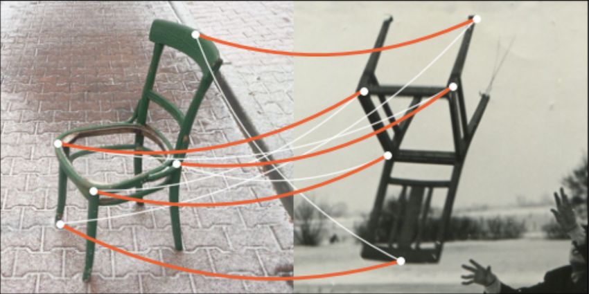
Module 1 CombOptNet
                                                                       function F ORWARD PASS(A, b, c)
                                                                         y := Solver(A, b, c)
                                                                         save y and A, b, c for backward pass
                                                                         return y
(a) yk0 is feasible but yk0 6= y.     (b) yk0 is infeasible.           function BACKWARD PASS(dy)
                                                                         load y and A, b, c P from forward pass
Figure 2: Geometric interpretation of the suggested con-                 Decompose dy = k λk ∆k
straint update. (a) All the constraints are satisfied for yk0 .            // set ∆k as in (9) and λk as in Proposition 1
The proxy minimizes the distance to the nearest (“most                   Calculate the gradients
active”) constraint to make y “less feasible”. A possible                            ∂P∆k            ∂P            ∂P
updated feasible region is shown in green. (b) The sug-                    dAk := ∂A       , dbk := ∂b∆k , dck := ∂c∆k
gested yk0 satisfies one of three constraints. The proxy                   // P∆k defined in (5) andP (7)
minimizes the distance to violated constraints to make yk0               Compose dA, db, dc := k λk dAk , dbk , dck
“more feasible”.                                                           // According to (6)
                                                                         return dA, db, dc
Note that our mapping dy 7→ dA, db is homogeneous. It
is due to the fact that the whole situation is rescaled to one
case (choice of basis) where the gradient is computed and An example of a decomposition is shown in Fig. 3. Further
then rescaled back (scalars λk ). The most natural scale discussion about the choice of basis and various compar-
agrees with the situation when the “targets” yk0 are the isons can be found in the Appendix.
closest integer neighbors. This ensures that the situation
does not collapse to a trivial solution (zero gradient) and,
simultaneously, that we do not interfere with very distant
values of y.
This basis selection plays a role of a “homogenizing hyper-
paramter” (λ in [41] or ε in [10]). In our case, we explicitly
construct a correct basis and do not need to optimize any
additional hyperparameter.

Cost update. Putting aside distinguishing of feasible and             Figure 3: All basis vectors ∆k (green) point more “towards
infeasible yk0 , the cost update problem has been addressed           the dy direction” compared to the canonical ones (orange).
in multiple previous works. We choose to use the simplest
approach of [19] and set
                                                             Constraint parametrization. For learning constraints,
                 c · ∆k if yk0 is feasible

  P∆k (c) =                                                  we have to specify their parametrization. The represen-
                                                            (7)
                 0         if yk0 is infeasible or yk0 ∈
                                                       / Y.  tation is of great importance, as it determines how the
The gradient dc is then composed analogously as in (6).      constraints respond to incoming gradients. Additionally, it
                                                             affects the meaning of constraint distance by changing the
The choice of the basis. Denote by k1 , . . . , kn the in- parameter space.
dices of the coordinates in the absolute values of dy in We represent each constraint (ak , bk ) as a hyperplane de-
decreasing order, i.e.                                       scribed by its normal vector ak , distance from the origin rk
                |dyk1 | ≥ |dyk2 | ≥ · · · ≥ |dykn |      (8) and offset ok of the origin in the global coordinate system
                                                             as displayed in Fig. 4a. Consequently bk = rk − ak · ok .
and set
                           k
                          X                                  Compared to the plain parametrization which represents
                   ∆k =       sign(dykj )ekj ,           (9) the constraints as a matrix A and a vector b, our slightly
                          j=1                                overparametrized choice allows the constraints to rotate
where ek is the k-th canonical vector. In other words, without requiring to traverse large distance in parame-
∆k is the (signed) indicator vector of the first k dominant ter space (consider e.g. a 180◦ rotation). An illustration
directions.                                                  is displayed in Fig. 4b. Comparison of our choice of
                                                             parametrization to other encodings and its effect on the
Denote by ` the largest index for which |dy` | > 0. Then
                                                             performance can be found in the Appendix.
the first ` vectors ∆k ’s are linearly independent and they
form a basis of the corresponding subspace. Therefore,
there exist scalars λk ’s satisfying (3).                    4 Demonstration & Analysis
Proposition 1. If λj = |dykj | − |dykj+1 | for j =
1, . . . , n − 1 and λn = |dykn |, then representation (3) We demonstrate the potential and flexibility of our method
holds with ∆k ’s as in (9).                                  on four tasks.

                                                                  4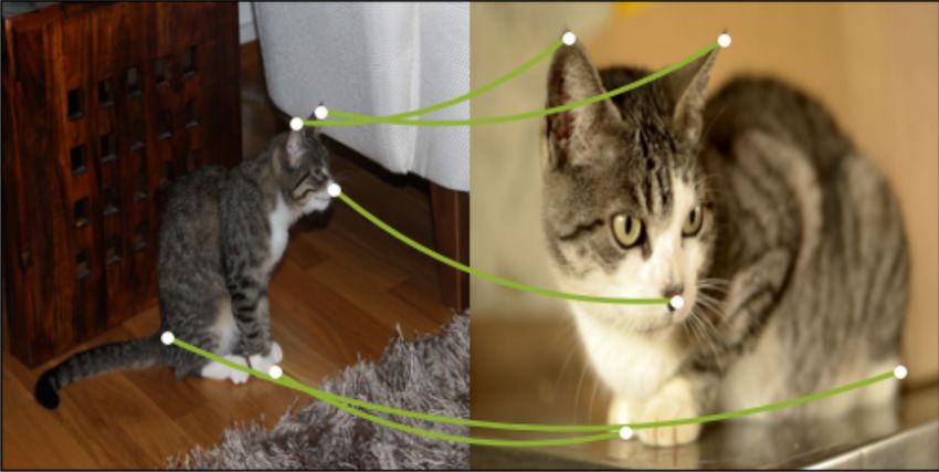
Each dataset fixes a set of (randomly chosen) constraints
                                                                      (A, b) specifying the ground-truth feasible region of an
                                                                      ILP solver. For the constraints (A, b) we then randomly
                                                                      sample cost vectors c and compute the corresponding ILP
                                                                      solution y ∗ (Fig. 5).

                                                                                             ILP Solver
 (a) Constraint representation   (b) Possible constraint update
Figure 4: (a) Each constraint (ak , bk ) is parametrized by Figure 5: Dataset generation for the RC demonstration.
its normal vector ak and a distance rk to its own origin ok .
                                                              The dataset consists of 1 600 pairs (c, y ∗ ) for training and
(b) Such a representation allows for easy rotations around
                                                              1 000 for testing. The solution space Y is either constrained
the learnable offset ok instead of rotating around the static
                                                              to [−5, 5]n (dense) or [0, 1]n (binary). During dataset
global origin.
                                                              generation, we performed a suitable rescaling to ensure a
Starting with an extensive performance analysis on syn- sufficiently large set of feasible solutions.
thetic data, we first demonstrate the ability to learn multiple
constraints simultaneously. For this, we learn a static set Architecture. The network learns the constraints (A, ∗b)
of randomly initialized constraints from solved instances, that specify the ILP solver from ground-truth pairs∗ (c, y ).
while using access to the ground-truth cost vector c.           Given c, predicted solution y is compared to y via the
                                                                MSE loss and the gradient is backpropagated to the learn-
Additionally, we show that the performance of our method able constraints using CombOptNet (Fig. 6).
on the synthetic datasets also translates to real classes of
ILPs. For this we consider a similarly structured task as
before, but use the NP-complete WSC problem to generate
the dataset.
Next, we showcase the ability to simultaneously learn the                        ILP Solver
full ILP specification. For this, we learn a single input-
dependent constraint and the cost vector jointly from the Figure 6: Architecture design for the RC demonstration.
ground truth solutions of KNAPSACK instances. These
instances are encoded as sentence embeddings of their The number of learned constraints matches the number of
description in natural language.                           constraints used for the dataset generation.
Finally, we demonstrate that our method is also applicable
to real-world problems. On the task of keypoint matching,             Baselines. We compare CombOptNet to three baselines.
we show that our method achieves results that are compa-              Agnostic to any constraints, a simple MLP baseline di-
rable to state-of-the-art architectures employing dedicated           rectly predicts the solution from the input cost vector as the
solvers. In this example, we jointly learn a static set of con-       integer-rounded output of a neural network. The CVXPY
straints and the cost vector from ground-truth matchings.             baseline uses an architecture similar to ours, only the Mod-
                                                                      ule 1 of CombOptNet is replaced with the CVXPY imple-
In all demonstrations, we use G UROBI [25] to solve the               mentation [15] of an LP solver that provides a backward
ILPs during training and evaluation. Implementation de-               pass proposed by Agrawal et al. [1]. Similar to our method,
tails, a runtime analysis and additional results, such as             it receives constraints and a cost vector and outputs the
ablations, other loss functions and more metrics, are pro-            solution of the LP solver greedily rounded to a feasible
vided in the Appendix. Additionally, a qualitative analysis           integer solution. Finally, we report the performance of
of the results for the Knapsack demonstration is included.            always producing the solution of the problem only con-
                                                                      strained to the outer region y ∈ Y . This baseline does
4.1   Random Constraints                                              not involve any training and is purely determined by the
                                                                      dataset.
Problem formulation. The task is to learn the con-
straints (A, b) corresponding to a fixed ILP. The network
                                                        Results. The results are reported in Fig. 7. In the bi-
has only access to the cost vectors c and the ground-truth
                                                        nary, case we demonstrate a high accuracy of perfectly
ILP solutions y ∗ . Note that the set of constraints perfectly
                                                        predicting the correct solution. The CVXPY baseline is
explaining the data does not need to be unique.         not capable of matching this, as it is not able to find a set
                                                        of constraints for the LP problem that mimics the effect
Dataset. We generate 10 datasets for each cardinality of running an ILP solver. For most cost vectors, CVXPY
m = 1, 2, 4, 8 of the ground-truth constraint set while often predicts the same solution as the unconstrained one
keeping the dimensionality of the ILP fixed to n = 16. and its ability to use constraints to improve is marginal.

                                                                  5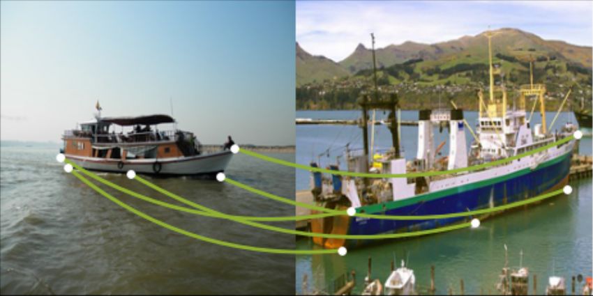
100                                                          we generate the dataset by solving instances of the NP-
                                           Box-constrained
                                                                 complete WSC problem.
     80                                    CombOptNet
                                           CVXPY
                                                                 Problem formulation. A family C of         Ssubsets of a uni-
     60                                    MLP
                                                                 verse U is called a covering of U if C = U . Given
                                                                 U = {1, . . . , m}, its covering C = {S1 , . . . , Sn } and cost
     40                                                          c : C → R, the task isP  to find the sub-covering C 0 ⊂ C with
                                                                 the lowest total cost S∈C 0 c(S).
     20
                                                                 The ILP formulation of this problem consists of m con-
      0                                                          straints in n dimensions. Namely, if y ∈ {0, 1}n denotes
              1           2           4            8             an indicator vector of the sets in C, akj = Jk ∈ Sj K and
             (a) Results on the binary datasets.                 bk = 1 for k = 1, . . . m, then the specification reads as
    100                                                                    X
                                           Box-constrained           min       c(Sj )yj      subject to      Ay ≥ b. (10)
                                                                     y∈Y
     80                                    CombOptNet                       j
                                           CVXPY
     60                                    MLP                   Dataset. We randomly draw n subsets from the m-
                                                                 element universe to form a covering C. To increase the vari-
     40                                                          ance of solutions, we only allow subsets with no more than
                                                                 3 elements. As for the Random Constraints demonstration,
     20                                                          the dataset consists of 1 600 pairs (c, y ∗ ) for training and
                                                                 1 000 for testing. Here, c is uniformly sampled positive
      0                                                          cost vector and y ∗ denotes the corresponding optimal so-
              1           2           4            8             lution (Fig. 8). We generate 10 datasets for each universe
              (b) Results on the dense datasets.                 size m = 4, 5, 6, 7, 8 with n = 2m subsets.
Figure 7: Results for the Random Constraints demonstra-
tion. We report mean accuracy (y = y ∗ in %) over 10                                  WSC Solver
datasets for 1, 2, 4 and 8 ground truth constraints in 16 di-
mensions. By Box-constrained we denote the performance
of always producing the solution of the problem only con- Figure 8: Dataset generation for the WSC demonstration.
strained to the outer region y ∈ Y , which does not involve
any training and is purely determined by the dataset.         Architecture and Baselines. We use the same architec-
                                                              ture and compare to the same baselines as in the Random
                                                              Constraints demonstration (Sec. 4.1).
The reason is that the LP relaxation of the ground truth
problem is far from tight and thus the LP solver proposes Results. The results are reported in Fig. 9. Our method is
many fractional solutions, which are likely to be rounded still able to predict the correct solution with high accuracy.
incorrectly. This highlights the increased expressivity of Compared to the previous demonstration, the performance
the ILP formulation compared to the LP formulation.           of the LP relaxation deteriorates. Contrary to the Ran-
Even though all methods decrease in performance in the dom Constraints datasets, the solution to the Weighted Set
dense case as the number of possible solutions is increased, Covering problem never matches the solution of the uncon-
the trend from the binary case continues. With the in- strained problem, which takes no subset. This prevents the
creased density of the solution space, the LP relaxation LP relaxation from exploiting these simple solutions and
becomes more similar to the ground truth ILP and hence ultimately leads to a performance drop. On the other hand,
the gap between CombOptNet and the CVXPY baseline the MLP baseline benefits from the enforced positivity of
decreases.                                                    the cost vector, which leads to an overall reduced number
                                                              of different solutions in the dataset.
We conclude that CombOptNet is especially useful, when
the underlying problem is truly difficult (i.e. hard to ap- 4.3 K NAPSACK from Sentence Description
proximate by an LP). This is not surprising, as CombOpt-
Net introduces structural priors into the network that are Problem formulation. The task is inspired by a vintage
designed for hard combinatorial problems.                     text-based PC game called “The Knapsack Problem” [35]
                                                              in which a collection of 10 items is presented to a player
                                                              including their prices and weights. The player’s goal is
4.2 Weighted Set Covering                                     to maximize the total price of selected items without ex-
                                                              ceeding the fixed 100-pound capacity of their knapsack.
We show that our performance on the synthetic datasets The aim is to solve instances of the NP-Hard K NAPSACK
also translates to traditional classes of ILPs. Considering a problem (2), from their word descriptions. Here, the cost
similarly structured architecture as in the previous section, c and the constraint (a, b) are learned simultaneously.

                                                             6
100                                                                    100
                                           Box-constrained
                                                                                  CombOptNet
                                           CombOptNet                             CVXPY
 80                                                                     80
                                           CVXPY                                  MLP
                                           MLP                          60        LPmax
 60

                                                                        40
 40
                                                                        20
 20
                                                                         0
                                                                              0     20         40     60       80      100
  0
           4           6           8           10                      (a) Evaluation accuracy (y = y ∗ in %) over training
                                                                       epochs. LPmax is the maximum achievable LP relaxation
Figure 9: Results of the WSC demonstration. We report                  accuracy.
mean accuracy (y = y ∗ in %) over 10 datasets for universe
sizes m = 4, 6, 8, 10 and 2m subsets.                                                                          CombOptNet
                                                                       0.20
                                                                                                               CVXPY
Dataset. Similarly to the game, a K NAPSACK instance                                                           MLP
consists of 10 sentences, each describing one item. The
sentences are preprocessed via the sentence embedding           0.10
[12] and the 10 resulting 4 096-dimensional vectors x con-
stitute the input of the dataset. We rely on the ability of     0.06
natural language embedding models to capture numerical
values, as the other words in the sentence are uncorrelated     0.04
with them (see an analysis of Wallace et al. [43]). The
                                                                      0       20       40        60      80  100
indicator vector y ∗ of the optimal solution (i.e. item se-
lection) to a knapsack instance is its corresponding label               (b) Training MSE  loss over epochs.
(Fig. 10). The dataset contains 4 500 training and 500 test Figure 12: Results or K NAPSACK demonstration. Reported
pairs (x, y ∗ ).                                            error bars are over 10 restarts.

                                                            Results. The results are presented in Fig. 12. While
                                                            CombOptNet is able to predict the correct items for the
                                                            K NAPSACK with good accuracy, the baselines are unable
                                                            to match this. Additionally, we evaluate the LP relaxation
Figure 10: Dataset generation for the K NAPSACK problem. on the ground truth weights and prices, providing an upper
                                                            bound for results achievable by any method relying on an
                                                            LP relaxation. The weak performance of this evaluation
Architecture. We simultaneously extract the learnable underlines the NP-Hardness of K NAPSACK. The ability
constraint coefficients (a, b) and the cost vector c via an to embed and differentiate through a dedicated ILP solver
MLP from the embedding vectors (Fig. 11).                   leads to surpassing this threshold even when learning from
                                                            imperfect raw inputs.

                                   ILP

                                                                 4.4     Deep Keypoint Matching

                                                             Problem formulation. Given are a source and target im-
Figure 11: Architecture design for the K NAPSACK prob- age showing an object of the same class (e.g. airplane),
lem.                                                         each labeled with a set of annotated keypoints (e.g. left
As only a single learnable constraint is used, which by wing). The task is to find the correct matching between the
definition defines a K NAPSACK problem, the interpreta- sets of keypoints from visual information without access
tion of this demonstration is a bit different from the other to the keypoint annotation. As not every keypoint has to
demonstrations. Instead of learning the type of combinato- be visible in both images, some keypoints can also remain
rial problem, we learn which exact K NAPSACK problem unmatched.
in terms of item-weights and knapsack capacity needs to As in this task the combinatorial problem is known a priori,
be solved.                                              state-of-the-art methods are able to exploit this knowledge
                                                        by using dedicated solvers. However, in our demonstration
Baselines. We compare to the same baselines as in the we make the problem harder by omitting this knowledge.
Random Constraints demonstration (Sec. 4.1).            Instead, we simultaneously infer the problem specification

                                                             7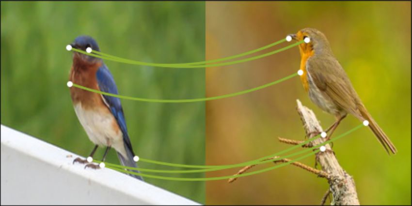
Table 1: Results for the keypoint matching demonstration.
Reported is the standard per-variable accuracy (%) metric
over 5 restarts. Column p × p corresponds to matching p
source keypoints to p target keypoints.
Method 4×4 5×5 6×6 7×7
CombOptNet 83.1 80.7 78.6 76.1
BB-GM 84.3 82.9 80.5 79.8
and train the feature extractor for the cost vector from data
end-to-end.
Dataset. We use the SPair-71k dataset [31] which was
published in the context of dense image matching and
was used as a benchmark for keypoint matching in recent
literature [37]. It includes 70 958 image pairs prepared
from Pascal VOC 2012 and Pascal 3D+ with rich pair-
level keypoint annotations. The dataset is split into 53 340
training pairs, 5 384 validation pairs and 12 234 pairs for
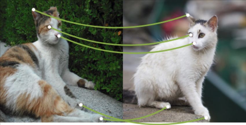
testing. Figure 13: Example matchings predicted by CombOptNet.
State-of-the-art. We compare to a state-of-the-art archi-
tecture BB-GM [37] that employs a dedicated solver for are especially satisfactory, considering the fact that BB-
the quadratic assignment problem. The solver is made GM outperforms the previous state-of-the-art architecture
differentiable with blackbox backpropagation [41], which [21] by several percentage points on experiments of this
allows to differentiate through the solver with respect to difficulty. Example matchings are shown in Fig. 13.
the input cost vector.
Architecture. We modify the BB-GM architecture by 5 Conclusion
replacing the blackbox-differentiation module employing
the dedicated solver with CombOptNet. We propose a method for integrating integer linear pro-
The drop-in replacement comes with a few important con- gram solvers into neural network architectures as layers.
siderations. Note that our method relies on a fixed di- This is enabled by providing gradients for both the cost
mensionality of the problem for learning a static (i.e. not terms and the constraints of an ILP. The resulting end-
input-dependent) constraint set. Thus, we can not learn an to-end trainable architectures are able to simultaneously
algorithm that is able to match any number of keypoints to extract features from raw data and learn a suitable set of
any other number of keypoints, as the dedicated solver in constraints that specify the combinatorial problem. Thus,
the baseline does. the architecture learns to fit the right NP-hard problem
needed to solve the task. In that sense, it strives to achieve
Due to this, we train four versions of our architecture, set- universal combinatorial expressivity in deep networks –
ting the number of keypoints in both source and target opening many exciting perspectives.
images to p = 4, 5, 6, 7. In each version, the dimensional-
ity is fixed to the number of edges in the bipartite graph. In the experiments, we demonstrate the flexibility of our
We use the same amount of learnable constrains as the num- approach, using different input domains, natural language
ber of ground-truth constraints that would realize the ILP and images, and different combinatorial problems with the
representation of the proposed mathching problem, i.e. the same CombOptNet module. In particular for combinatori-
combined number of keypoints in both images (m = 2p). ally hard problems we see a strong advantage of the new
architecture.
The randomly initialized constraint set and the backbone
architecture that produces the cost vectors c are learned The potential of our method is highlighted by the demon-
simultaneously from pairs of predicted solutions y and stration on the keypoint matching benchmark. Unaware
ground-truth matchings y ∗ using CombOptNet. of the underlying combinatorial problem, CombOptNet
achieves a performance that is not far behind architectures
employing dedicated state-of-the-art solvers.
Results. The results are presented in Tab. 1. Even though
CombOptNet is uninformed about which combinatorial In future work we aim to make the number of constraints
problem it should be solving, its performance is close to the flexible and to explore more problems with hybrid combi-
privileged state-of-the-art method BB-GM. These results natorial complexity and statistical learning aspects.
8A Demonstrations of 512, ReLU nonlinearity on the hidden nodes, and a sig-
moid nonlinearity on the output. The output is scaled to
A.1 Implementation Details the ground-truth price range [10, 45] for the cost c and to
the ground-truth weight range [15, 35] for the constraint
When learning multiple constraints, we replace the mini- a. The bias term is fixed to the ground-truth knapsack
mum in definition (5) of mismatch function P∆k with its capacity b = 100. Item weights and prices as well as the
softened version. Therefore, not only the single closest knapsack capacity are finally multiplied by a factor of 0.01
constraint will shift towards yk0 , but also other constraints to produce a reasonable scale for the constraint parameters
close to yk0 will do. For the softened minimum we use and cost vector.
X x
k The CVXPY baseline implements a greedy rounding pro-
softmin(x) = −τ · log exp − , (A1) cedure to ensure the feasibility of the predicted integer
τ
k solution with respect to the learned constraints. Starting
which introduces the temperature τ , determining the soft- from the item with the largest predicted (noninteger) value,
ening strength. the procedure adds items to the predicted (integer) solution
until no more items can be added without surpassing the
In all experiments, we normalize the cost vector c before
knapsack capacity.
we forward it to the CombOptNet module. For the loss we
use the mean squared error between the normalized pre- The MLP baseline employs an MLP consisting of three
dicted solution y and the normalized ground-truth solution layers with dimensionality 100 and ReLU activation on the
y ∗ . For normalization we apply the shift and scale that hidden nodes. Without using an output nonlinearity, the
translates the underlying hypercube of possible solutions output is rounded to the nearest integer point to obtain the
([0, 1]n in binary or [−5, 5]n in dense case) to a normalized predicted solution.
hypercube [−0.5, 0.5]n .
The hyperparameters for all demonstrations are listed in Deep Keypoint Matching. We initialize a set of con-
Tab. A1. We use Adam [27] as the optimizer for all demon- straints exactly as in the binary case of the Random Con-
strations. straints demonstration. We use the architecture described
by Rolínek et al. [37], only replacing the dedicated solver
Random Constraints. For selecting the set of con- module with CombOptNet.
straints for data generation, we uniformly sample con-
straint origins ok in the center subcube (halved edge We train models for varying numbers of keypoints p =
length) of the underlying hypercube of possible solutions. 4, 5, 6, 7 in the source and 2
target image, resulting in varying
The constraint normals ak and the cost vectors c are ran- dimensionalities n = p and number of constraints m =
domly sampled normalized vectors and the bias terms are 2p. Consistent with Rolínek et al. [37], all models are
initially set to bk = 0.2. The signs of the constraint nor- trained for 10 epochs, each consisting of 400 iterations
mals ak are flipped in case the origin is not feasible, ensur- with randomly drawn samples from the training set. We
ing that the problem has at least one feasible solution. We discard samples with fewer keypoints than what is specified
generate 10 such datasets for m = 1, 2, 4, 8 constraints in for the model through the dimensionality of the constraint
n = 16 dimensions. The size of each dataset is 1 600 train set. If the sample has more keypoints, we chose a random
instances and 1 000 test instances. subset of the correct size.
For learning, the constraints are initialised in the same way After each epoch, we evaluate the trained models on the
except for the feasibility check, which is skipped since validation set. Each model’s highest-scoring validation
CombOptNet can deal with infeasible regions itself. stage is then evaluated on the test set for the final results.
K NAPSACK from Sentence Description. Our method
and CVXPY use a small neural network to extract weights A.2 Runtime analysis.
and prices from the 4 096-dimensional embedding vec-
tors. We use a two-layer MLP with a hidden dimension The runtimes of our demonstrations are reported in Tab. A2.
Random Constrains demonstrations have the same run-
Table A1: Hyperparameters for all demonstrations. times as Weighted Set Covering since they share the archi-
tecture.
WSC & Random Keypoint
Knapsack Unsurprisingly, CombOptNet has higher runtimes as it re-
Constraints Matching
lies on ILP solvers which are generally slower than LP
Learning rate 5 × 10⁻⁴ 5 × 10⁻⁴ 1 × 10⁻⁴ solvers. Also, the backward pass of CombOptNet has neg-
Batch size 8 8 8 ligible runtime compared to the forward-pass runtime. In
Train epochs 100 100 10 Random Constraints, Weighted Set Covering and K NAP -
τ 0.5 0.5 0.5 SACK demonstration, the increased runtime is necessary,
Backbone lr – – 2.5 × 10⁻⁶ as the baselines simply do not solve a hard enough problem
to succeed in the tasks.
9Table A2: Average runtime for training and evaluating a Table A4: Weighted set covering demonstration with mul-
model on a single Tesla-V100 GPU. For Keypoint Match- tiple learnable constraints.
ing, the runtime for the largest model (p = 7) is shown.
k 4 6 8 10
Weighted Keypoint ?
Knapsack 1 100 ± 0.0 97.2 ± 6.4 79.7 ± 12.1 56.7 ± 14.8
Set Covering Matching
2 100 ± 0.0 99.5 ± 1.9 99.3 ± 0.8 80.4 ± 13.0
CombOptNet 1h 30m 3h 50m 5h 30m 4 100 ± 0.0 99.9 ± 0.0 97.9 ± 6.4 85.2 ± 8.1
CVXPY 1h 2h 30m –
MLP 10m 20m – Table A5: Random Constraints dense demonstration with
BB-GM – – 55m various loss functions. For the Huber loss we set β = 0.3.
Statistics are over 20 restarts (2 for each of the 10 dataset
Table A3: Random Constraints demonstration with multi- seeds).
ple learnable constraints. Using a dataset with m ground-
truth constraints, we train a model with k × m learnable Loss 1 2 4 8
constraints. Reported is evaluation accuracy (y = y ∗ in ?
MSE 87.3 ± 2.5 70.2 ± 11.6 29.6 ± 10.4 2.3 ± 1.2
%) for m = 1, 2, 4, 8. Statistics are over 20 restarts (2 for
Huber 88.3 ± 4.0 75.4 ± 9.3 25.0 ± 11.8 2.6 ± 2.7
each of the 10 dataset seeds).
L0 85.9 ± 3.4 65.8 ± 3.5 15.3 ± 4.3 1.1 ± 0.3
m 1 2 4 8 L1 89.2 ± 1.6 75.8 ± 10.8 30.2 ± 16.5 2.1 ± 1.2
1 × m? 97.8 ± 0.7 94.2 ± 10.1 77.4 ± 13.5 46.5 ± 12.4
binary
2 × m 97.3 ± 0.9 95.1 ± 1.6 87.8 ± 5.2 63.1 ± 7.0 number of learnable constraints. The results are listed in
4 × m 96.9 ± 0.7 95.1 ± 1.2 88.7 ± 2.3 77.7 ± 3.2
Tab. A6. Similar to the binary Random Constraints ab-
lation with m = 1, increasing the number of learnable
1 × m? 87.3 ± 2.5 70.2 ± 11.6 29.6 ± 10.4 2.3 ± 1.2 constraints does not result in strongly increased perfor-
dense
2 × m 87.8 ± 1.7 73.4 ± 2.4 32.7 ± 7.6 2.4 ± 0.8 mance.
4 × m 85.0 ± 2.6 64.6 ± 3.9 28.3 ± 2.7 2.9 ± 1.3
Additionally, we provide a qualitative analysis of the re-
In the Keypoint Matching demonstration, CombOptNet sults on the K NAPSACK task. In Fig. A1 we compare
slightly drops behind BB-GM and requires higher runtime. the total ground-truth price of the predicted instances to
Such drawback is outweighed by the benefit of employing the total price of the ground-truth solutions on a single
a broad-expressive model that operates without embedded evaluation of the trained models.
knowledge of the underlying combinatorial task. The plots show that CombOptNet is achieving much better
results than CVXPY. The total prices of the predictions are
A.3 Additional Results very close to the optimal prices and only a few predictions
are infeasible, while CVXPY tends to predict infeasible
Random Constraints & Weighted Set Covering. We solutions and only a few predictions have objective values
provide additional results regarding the increased amount matching the optimum.
of learned constraints in Tab. A3 and A4) and the choice
of the loss function Tab. A5. In Fig. A2 we compare relative errors on the individual
item weights and prices on the same evaluation of the
With a larger set of learnable constraints the model is able trained models as before. Since (I)LP costs are scale invari-
to construct a more complex feasible region. While in gen- ant, we normalize predicted price vector to match the size
eral this tends to increase performance and reduce variance of the ground-truth price vector before the comparison.
by increasing robustness to bad initializations, it can also
lead to overfitting similarly to a neural net with too many CombOptNet shows relatively small normally distributed
parameters. errors on both prices and weights, precisely as expected
from the prediction of a standard network. CVXPY reports
In the dense case, we also compare different loss functions much larger relative errors on both prices and weights
which is possible because CombOptNet can be used as (note the different plot scale). The vertical lines correspond
an arbitrary layer. As shown in Tab. A5, this choice mat- to the discrete steps of ground-truth item weights in the
ters, with the MSE loss, the L1 loss and the Huber loss dataset. Unsurprisingly, the baseline usually tends to either
outperforming the L0 loss. This freedom of loss function
choice can prove very helpful for training more complex Table A6: Knapsack demonstration with more learnable
architectures. constraints. Reported is evaluation accuracy (y = y ∗ in
%) for m = 1, 2, 4, 8 constraints. Statistics are over 10
restarts.
K NAPSACK from Sentence Description. As for the
Random Constraints demonstration, we report the perfor- 1? 2 4 8
mance of CombOptNet on the K NAPSACK task for a higher
? 64.7 ± 2.8 63.5 ± 3.7 65.7 ± 3.1 62.6 ± 4.4
Used in the main demonstrations.
10Price of pred. solution descent direction. As a result, the gradient computation
leads to updates that are very detached from the original
200 200 incoming gradient.
Finally, the softened minimum leads to increased perfor-
150 150
mance in all demonstrations. This effect is apparent par-
optimal
ticularly in the case of a binary solution space, as the
feasible
100 100 constraints can have a relevant impact on the predicted
infeasible
solution y over large distances. Therefore, only updating
100 150 200 100 150 200 the constraint which is closest to the predicted solution y,
Price of GT solution Price of GT solution as it is the case for a hard minimum, gives no gradient to
(a) CombOptNet (b) CVXPY constraints that may potentially have had a huge influence
Figure A1: Prices analysis for the K NAPSACK demonstra- on y.
tion. For each test set instance, we plot the total price of the
predicted solution over the total price of the ground-truth B Method
solution. Predicted solutions which total weight exceeds
the knapsack capacity are colored in red (cross).
To recover the situation from the method section, set x as
feasible one of the inputs A, b, or c.
0.2
Relative price error
0.5 infeasible Proposition A1. Let y : R` → Rn be differentiable
at x ∈ R` and let L : Rn → R be differentiable at
0.0 0.0 y = y(x) ∈ Rn . Denote dy = ∂L/∂y at y. Then the
distance between y(x) and y − dy is minimized along the
−0.5 direction ∂L/∂x, where ∂L/∂x stands for the derivative
−0.2 of L(y(x)) at x.
−0.2 0.0 0.2 −0.5 0.0 0.5
Relative weight error Relative weight error Proof. For ξ ∈ R` , let ϕ(ξ) denote the distance between
(a) CombOptNet (b) CVXPY y(x − ξ) and the target y(x) − dy, i.e.
Figure A2: Qualitative analysis of the errors on weights ϕ(ξ) = y(x − ξ) − y(x) + dy .
and prices in the K NAPSACK demonstration. We plot
the relative error between predicted and ground-truth item There is nothing to prove when dy = 0 as y(x) = y − dy
prices over the relative error between predicted and ground- and there is no room for any improvement. Otherwise, ϕ is
truth item weights. Colors denote whether the predicted positive and differentiable in a neighborhood of zero. The
solution is feasible in terms of ground-truth weights. Fréchet derivative of ϕ reads as
∂y
overestimate the price and underestimate the item weight, 0 − y(x − ξ) − y(x) + dy · ∂x (x − ξ)
ϕ (ξ) = ,
or vice versa, due to similar effects of these errors on the y(x − ξ) − y(x) + dy
predicted solution.
whence
A.4 Ablations 1 ∂L ∂y 1 ∂L
ϕ0 (0) = − · =− , (A2)
kdyk ∂y ∂x kdyk ∂x
We ablate the choices in our architecture and model design
on the Random Constraints (RC) and Weighted Set Cover- where the last equality follows by the chain rule. Therefore,
ing (WSC) tasks. In Tab. A7 and A8 we report constraint the direction of the steepest descent coincides with the
parametrization, choice of basis, and minima softening direction of the derivative ∂L/∂x, as kdyk is a scalar.
ablations.
proof of Proposition 1. We prove that
The ablations show that our parametrization with learn-
able origins is consistently among the best ones. Without X n Xn `−1
X
learnable origins, the performance is highly dependend on u e
j kj = λ ∆
j j − |u` | sign(uj )ekj (A3)
the origin of the coordinate system in which the directly j=` j=` j=1
learned parameters (A, b) are defined.
for every ` = 1, . . . , n, where we abbreviate uj = dykj .
The choice of basis in the gradient decomposition shows The claimed equality (3) then follows from (A3) in the
a large impact on performance. Our basis ∆ (9) is out- special case ` = 1.
performing the canonical one in the binary RC and WSC
demonstration, while showing performance similar to the We proceed by induction. In the first step we show (A3)
canonical basis in the dense RC case. The canonical basis for ` = n. Definition n−1
of ∆n (9) yields
0
X
produces directions for the computation of yk that in many λn ∆n − |un | sign(uj )ekj
cases point in very different directions than the incoming j=1
11Table A7: Ablations of CombOptNet on Random Constraints demonstration. Reported is
evaluation accuracy (y = y ∗ in %) for m = 1, 2, 4, 8 ground-truth constraints. Statistics
are over 20 restarts (2 for each of the 10 dataset seeds).
Method 1 2 4 8
?
learnable origins 97.8 ± 0.7 94.2 ± 10.1 77.4 ± 13.5 46.5 ± 12.4
param.
direct (origin at corner) 97.4 ± 1.0 94.9 ± 7.0 59.0 ± 26.8 26.9 ± 10.3
direct (origin at center) 98.0 ± 0.5 97.1 ± 0.6 70.5 ± 19.1 44.6 ± 5.9
binary
∆ basis?
basis
97.8 ± 0.7 94.2 ± 10.1 77.4 ± 13.5 46.5 ± 12.4
canonical 96.3 ± 1.9 70.8 ± 4.1 14.4 ± 3.2 2.7 ± 0.9
hard 83.1 ± 13.2 55.4 ± 18.9 37.7 ± 8.7
min
soft (τ = 0.5)? 97.8 ± 0.7 94.2 ± 10.1 77.4 ± 13.5 46.5 ± 12.4
soft (τ = 1.0) 95.7 ± 2.2 70.2 ± 14.1 36.0 ± 9.7
learnable origins? 87.3 ± 2.5 70.2 ± 11.6 29.6 ± 10.4 2.3 ± 1.2
param.
direct (origin at corner) 86.7 ± 3.0 74.6 ± 3.6 32.6 ± 13.7 2.8 ± 0.5
direct (origin at center) 83.0 ± 6.1 43.8 ± 13.2 11.6 ± 3.1 1.1 ± 0.5
dense
∆ basis?
basis
87.3 ± 2.5 70.2 ± 11.6 29.6 ± 10.4 2.3 ± 1.2
canonical 88.6 ± 1.4 71.6 ± 1.6 26.8 ± 4.1 4.0 ± 0.7
hard 70.8 ± 15.1 21.4 ± 10.7 2.2 ± 2.1
min
soft (τ = 0.5)? 89.1 ± 2.8 70.2 ± 11.6 29.6 ± 10.4 2.3 ± 1.2
soft (τ = 1.0) 73.0 ± 12.1 31.9 ± 11.7 2.2 ± 1.5
Table A8: Ablations of CombOptNet on Weighted Set Covering. Reported is evaluation
accuracy (y = y ∗ in %) for m = 4, 6, 8, 10 ground-truth constraints.
Method 4 6 8 10
?
learnable origins 100 ± 0.0 97.2 ± 6.4 79.7 ± 12.1 56.7 ± 14.8
param.
direct (origin at corner) 99.4 ± 2.9 94.1 ± 16.4 78.5 ± 15.7 47.7 ± 17.9
direct (fixed origin at 0) 99.9 ± 0.6 87.6 ± 6.4 65.3 ± 11.9 46.7 ± 11.5
∆ basis?
basis
100 ± 0.0 97.2 ± 6.4 79.7 ± 12.1 56.7 ± 14.8
canonical 8.4 ± 13.3 2.0 ± 2.6 0.2 ± 0.3 0.0 ± 0.1
hard 88.2 ± 13.4 64.3 ± 14.6 45.1 ± 14.1 32.3 ± 17.4
soft (τ = 0.5)? 100 ± 0.0 97.2 ± 6.4 79.7 ± 12.1 56.7 ± 14.8
min
soft (τ = 1.0) 99.9 ± 0.4 95.6 ± 9.6 70.3 ± 15.5 51.2 ± 16.4
soft (τ = 2.0) 98.8 ± 3.1 90.6 ± 14.3 66.4 ± 12.5 51.2 ± 9.5
soft (τ = 5.0) 97.5 ± 11.1 90.2 ± 9.1 64.2 ± 11.8 49.7 ± 10.4
n
X n−1
X `
X `−1
X
= |un | sign(uj )ekj − |un | sign(uj )ekj + |u`+1 | sign(uj )ekj − |u` | sign(uj )ekj
j=1 j=1 j=1 j=1
= un ekn . n
X `
X
= uj ekj + |u` | − |u`+1 | sign(uj )ekj
Now, assume that (A3) holds for ` + 1 ≥ 2. We show that j=`+1 j=1
(A3) holds for ` as well. Indeed, `
X `−1
X
+ |u`+1 | sign(uj )ekj − |u` | sign(uj )ekj
n `−1
X X j=1 j=1
λj ∆j − |u` | sign(uj )ekj n n
X X
j=` j=1 = uj ekj + sign(u` )|u` |ek` = uj ekj ,
n
X `
X j=`+1 j=`
= λj ∆j − |u`+1 | sign(uj )ekj + λ` ∆`
j=`+1 j=1 where we used the definitions of ∆` and λ` .
12References language inference data. In Conference on Empiri-
cal Methods in Natural Language Processing, pages
[1] Akshay Agrawal, Brandon Amos, Shane Barratt, 670–680, Copenhagen, Denmark, 2017. Association
Stephen Boyd, Steven Diamond, and J Zico Kolter. for Computational Linguistics.
Differentiable convex optimization layers. In Ad-
vances in Neural Information Processing Systems, [13] IBM ILOG Cplex. V12. 1: User’s Manual for
pages 9562–9574, 2019. CPLEX. International Business Machines Corpo-
[2] Akshay Agrawal, Shane Barratt, Stephen Boyd, Enzo ration, 46(53):157, 2009.
Busseti, and Walaa M. Moursi. Differentiating [14] Gal Dalal, Krishnamurthy Dvijotham, Matej Ve-
through a cone program. J. Appl. Numer. Optim, cerik, Todd Hester, Cosmin Paduraru, and Yuval
1(2):107–115, 2019. Tassa. Safe exploration in continuous action spaces.
[3] Brandon Amos. Differentiable optimization-based arXiv:1801.08757, 2018.
modeling for machine learning. PhD thesis, PhD [15] Steven Diamond and Stephen Boyd. CVXPY: A
thesis. Carnegie Mellon University, 2019. Python-embedded modeling language for convex op-
[4] Brandon Amos and J Zico Kolter. Optnet: Differ- timization. Journal of Machine Learning Research,
entiable optimization as a layer in neural networks. 17(83):1–5, 2016.
In International Conference on Machine Learning,
[16] Josip Djolonga and Andreas Krause. Differentiable
pages 136–145, 2017.
learning of submodular models. In Advances in
[5] Brandon Amos and Denis Yarats. The differentiable Neural Information Processing Systems, pages 1013–
cross-entropy method. In International Conference 1023, 2017.
on Machine Learning, pages 291–302, 2020.
[17] Justin Domke. Generic methods for optimization-
[6] Maria-Florina Balcan, Travis Dick, Tuomas Sand- based modeling. In Artificial Intelligence and Statis-
holm, and Ellen Vitercik. Learning to branch. In tics, pages 318–326, 2012.
International conference on machine learning, pages
344–353, 2018. [18] Priya Donti, Brandon Amos, and J Zico Kolter. Task-
based end-to-end model learning in stochastic opti-
[7] Mislav Balunovic, Pavol Bielik, and Martin Vechev.
mization. In Advances in Neural Information Pro-
Learning to solve SMT formulas. In Advances in Neu-
cessing Systems, pages 5484–5494, 2017.
ral Information Processing Systems, pages 10317–
10328, 2018. [19] Adam N. Elmachtoub and Paul Grigas. Smart “pre-
[8] Peter Battaglia, Jessica Blake Chandler Hamrick, Vic- dict, then optimize”. arXiv:1710.08005, 2020.
tor Bapst, Alvaro Sanchez, Vinicius Zambaldi, Ma- [20] Aaron Ferber, Bryan Wilder, Bistra Dilkina, and
teusz Malinowski, Andrea Tacchetti, David Raposo, Milind Tambe. MIPaaL: Mixed integer program as a
Adam Santoro, Ryan Faulkner, Caglar Gulcehre, layer. In AAAI Conference on Artificial Intelligence,
Francis Song, Andy Ballard, Justin Gilmer, George E. volume 34, pages 1504–1511, 2020.
Dahl, Ashish Vaswani, Kelsey Allen, Charles Nash,
Victoria Jayne Langston, Chris Dyer, Nicolas Heess, [21] Matthias Fey, Jan E Lenssen, Christopher Morris,
Daan Wierstra, Pushmeet Kohli, Matt Botvinick, Jonathan Masci, and Nils M Kriege. Deep graph
Oriol Vinyals, Yujia Li, and Razvan Pascanu. Re- matching consensus. In International Conference on
lational inductive biases, deep learning, and graph Learning Representations, 2020.
networks. arXiv:1806.01261, 2018. [22] Stephen Gould, Basura Fernando, Anoop Cherian,
[9] Irwan Bello, Hieu Pham, Quoc V Le, Moham- Peter Anderson, Rodrigo Santa Cruz, and Edison
mad Norouzi, and Samy Bengio. Neural combi- Guo. On differentiating parameterized argmin and
natorial optimization with reinforcement learning. argmax problems with application to bi-level opti-
arXiv:1611.09940, 2016. mization. arXiv:1607.05447, 2016.
[10] Quentin Berthet, Mathieu Blondel, Olivier Teboul, [23] Alex Graves, Greg Wayne, and Ivo Danihelka. Neural
Marco Cuturi, Jean-Philippe Vert, and Francis Bach. turing machines. arXiv:1410.5401, 2014.
Learning with differentiable perturbed optimizers. In
Advances in Neural Information Processing Systems, [24] Alex Graves, Greg Wayne, Malcolm Reynolds,
pages 9508–9519, 2020. Tim Harley, Ivo Danihelka, Agnieszka Grabska-
Barwińska, Sergio Gómez Colmenarejo, Edward
[11] Luca Bertinetto, Joao F Henriques, Philip HS Torr, Grefenstette, Tiago Ramalho, John Agapiou,
and Andrea Vedaldi. Meta-learning with differen- Adrià Puigdomènech Badia, Karl Moritz Hermann,
tiable closed-form solvers. In International Confer- Yori Zwols, Georg Ostrovski, Adam Cain, Helen
ence on Learning Representations, 2019. King, Christopher Summerfield, Phil Blunsom, Ko-
[12] Alexis Conneau, Douwe Kiela, Holger Schwenk, ray Kavukcuoglu, and Demis Hassabis. Hybrid com-
Loïc Barrault, and Antoine Bordes. Supervised learn- puting using a neural network with dynamic external
ing of universal sentence representations from natural memory. Nature, 538(7626):471–476, October 2016.
13[25] LLC Gurobi Optimization. Gurobi optimizer ref- [37] Michal Rolínek, Paul Swoboda, Dominik Zietlow,
erence manual, 2019. URL http://www.gurobi. Anselm Paulus, Vít Musil, and Georg Martius. Deep
com. graph matching via blackbox differentiation of com-
[26] Elias Khalil, Hanjun Dai, Yuyu Zhang, Bistra Dilkina, binatorial solvers. In European Conference on Com-
and Le Song. Learning combinatorial optimization puter Vision, pages 407–424, 2020.
algorithms over graphs. In Advances in Neural Infor- [38] Yingcong Tan, Daria Terekhov, and Andrew Delong.
mation Processing Systems, pages 6348–6358, 2017. Learning linear programs from optimal decisions. In
[27] Diederik P. Kingma and Jimmy Ba. Adam: A method Advances in Neural Information Processing Systems,
for stochastic optimization. In International Confer- pages 19738–19749, 2020.
ence on Learning Representations, 2014.
[39] Petar Veličković, Guillem Cucurull, Arantxa
[28] Wouter Kool, Herke van Hoof, and Max Welling. Casanova, Adriana Romero, Pietro Lio, and Yoshua
Attention, learn to solve routing problems! In In- Bengio. Graph attention networks. In International
ternational Conference on Learning Representations, Conference on Learning Representations, 2018.
2018.
[40] Petar Veličković, Rex Ying, Matilde Padovano, Raia
[29] Kwonjoon Lee, Subhransu Maji, Avinash Ravichan- Hadsell, and Charles Blundell. Neural execution of
dran, and Stefano Soatto. Meta-learning with differ- graph algorithms. In International Conference on
entiable convex optimization. In Conference on Com- Learning Representations, 2020.
puter Vision and Pattern Recognition, pages 10657–
10665, 2019. [41] M. Vlastelica, A. Paulus, V. Musil, G. Martius, and
M. Rolínek. Differentiation of blackbox combinato-
[30] Chun Kai Ling, Fei Fang, and J Zico Kolter. What
rial solvers. In International Conference on Learning
game are we playing? End-to-end learning in normal
Representations, 2020.
and extensive form games. In International Joint
Conference on Artificial Intelligence, 2018. [42] Marin Vlastelica, Michal Rolinek, and Georg Mar-
[31] Juhong Min, Jongmin Lee, Jean Ponce, and Minsu tius. Discrete planning with end-to-end trained neuro-
Cho. SPair-71k: A Large-scale Benchmark for Se- algorithmic policies. ICML 2020, Graph Representa-
mantic Correspondence. arXiv:1908.10543, 2019. tion Learning Workshop, 2020.
[32] Vinod Nair, Sergey Bartunov, Felix Gimeno, In- [43] Eric Wallace, Yizhong Wang, Sujian Li, Sameer
grid von Glehn, Pawel Lichocki, Ivan Lobov, Bren- Singh, and Matt Gardner. Do NLP models know
dan O’Donoghue, Nicolas Sonnerat, Christian Tjan- numbers? Probing numeracy in embeddings. In Con-
draatmadja, Pengming Wang, Ravichandra Addanki, ference on Empirical Methods in Natural Language
Tharindi Hapuarachchi, Thomas Keck, James Keel- Processing and the 9th International Joint Confer-
ing, Pushmeet Kohli, Ira Ktena, Yujia Li, Oriol ence on Natural Language Processing, pages 5310–
Vinyals, and Yori Zwols. Solving mixed integer pro- 5318, 2019.
grams using neural networks. arXiv:2012.13349,
2020. [44] Po-Wei Wang, Priya Donti, Bryan Wilder, and Zico
Kolter. SATNet: Bridging deep learning and logical
[33] Mohammadreza Nazari, Afshin Oroojlooy, Lawrence reasoning using a differentiable satisfiability solver.
Snyder, and Martin Takác. Reinforcement learning In International Conference on Machine Learning,
for solving the vehicle routing problem. In Advances pages 6545–6554, 2019.
in Neural Information Processing Systems, pages
9839–9849, 2018. [45] Bryan Wilder, Eric Ewing, Bistra Dilkina, and Milind
Tambe. End to end learning and optimization on
[34] Vlad Niculae, Andre Martins, Mathieu Blondel, and graphs. In Advances in Neural Information Process-
Claire Cardie. Sparsemap: Differentiable sparse ing Systems, pages 4672–4683, 2019.
structured inference. In International Conference
on Machine Learning, pages 3799–3808, 2018. [46] Andrei Zanfir and Cristian Sminchisescu. Deep learn-
[35] Leonard Richardson. The knapsack problem, the ing of graph matching. In Conference on Computer
game of premature optimization, 2001. URL https: Vision and Pattern Recognition, pages 2684–2693,
//www.crummy.com/software/if/knapsack/. 2018.
[36] M. Rolínek, V. Musil, A. Paulus, M. Vlastelica, [47] Wei Zhang and Thomas G Dietterich. Solving com-
C. Michaelis, and G. Martius. Optimizing ranking- binatorial optimization tasks by reinforcement learn-
based metrics with blackbox differentiation. In Con- ing: A general methodology applied to resource-
ference on Computer Vision and Pattern Recognition, constrained scheduling. Journal of Artificial Intelli-
2020. gence Reseach, 1:1–38, 2000.
14You can also read