Artificial Intelligence Inspired Self-Deployment of Wireless Networks
←
→
Page content transcription
If your browser does not render page correctly, please read the page content below
Artificial Intelligence Inspired Self-Deployment of
                                                             Wireless Networks
                                                                                   Erma Perenda∗ , Ramy Atawia† and Haris Gacanin†
                                                                                                   ∗ NokiaShanghai Bell, China
                                                                               † Nokia   Bell Labs, Belgium, haris.gacanin@nokia-bell-labs.com

                                            Abstract—In this paper, we propose a self-deployment ap-                      This paper, for the first time in literature, introduces an arti-
                                         proach for finding the optimal placement of extenders in which                ficial intelligence (AI) case based reasoning (CBR) framework
arXiv:1805.06217v1 [cs.NI] 16 May 2018

                                         both the wireless back-haul and front-haul throughput of the                  for self-deployment of wireless network2 . The framework
                                         extender are optimized. We present an artificial intelligence (AI)
                                         case based reasoning (CBR) framework that enables autonomous                  enables network to sense the environment and build necessary
                                         self-deployment in which the network can learn the environment                knowledge used to 1) assess the optimality of current position
                                         by means of sensing and perception. New actions, i.e. extender                and 2) propose new locations for EXTs. We design framework
                                         positions, are created by problem-specific optimization and semi-             to ubiquitously monitor the user satisfaction and determine the
                                         supervised learning algorithms that balance exploration and                   optimality of current location. The network notifies the user
                                         exploitation of the search space. An IEEE 802.11 standard
                                         compliant simulations are performed to evaluate the framework                 to reposition an EXT to optimal location with guaranteed de-
                                         on a large scale and compare its performance against existing                 mand. The main contributions of this paper can be summarized
                                         conventional coverage maximization approaches. Experimental                   as follows:
                                         evaluation is also performed in an enterprise environment to
                                                                                                                          • We propose a general AI framework for self-deployment
                                         demonstrate the competence of the proposed AI-framework in
                                         perceiving such a dense scenario and reason the extender deploy-                    of wireless network based on CBR. The previous network
                                         ment that achieves user quality of service (QoS). Throughput                        states, optimization actions and rewards are frequently
                                         fairness and ubiquitous QoS satisfaction are achieved which                         stored in the knowledge base (KB), and then used to guide
                                         provide a leap to apply AI-driven self-deployment in wireless                       the network while taking future decisions.
                                         networks.
                                                                                                                          • A problem-specific optimization with active learning is
                                            Index Terms—Artificial intelligence, optimization, wireless net-
                                         work.                                                                               introduced to populate the KB with actions and their
                                                                                                                             corresponding fitness values. This is done while tackling
                                                                                                                             the search trade-off between exploitation and exploration.
                                                                  I. I NTRODUCTION                                           Hence, avoids trapping the search at local optimal solu-
                                            IEEE 802.11 wireless network is expected to serve more                           tions and prevent the network from revisiting discovered
                                         than 50% of the global data traffic in 2021 [1]. Such a                             search space. Such methodology increases the chance of
                                         network will thus employ a large number of access points                            reaching optimal position of extenders at low searching
                                         (APs) with wired backhaul1 , more than half billion, that are                       and learning costs.
                                         deployed in dynamic manner. At the same time, connectivity                       • To speed up learning and minimize the cost of learning

                                         nodes having a wireless back-haul, referred to as extenders                         we introduce semi-supervised learning to learn and adjust
                                         (EXTs), are flooding the wireless indoor market to minimize                         system variables (i.e. throughput) and exploration factor
                                         the deployment cost and improve coverage [2]. Thus, shifting                        that controls optimization process – more robust explo-
                                         to multi-hop architectures, but increasing interference and                         ration and exploitation strategy. We introduce support
                                         contention [3]. The main challenge in such deployments is                           vector machine (SVM) estimation of throughput variables
                                         the lack of coordination between mAP and EXT serving                                when non-empty set of training data is present.
                                         overlapping areas, and shared unlicenced spectrum by different                   • We introduce the first testbed that integrates AI in

                                         network operators. New deployment strategy is crucial to                            wireless network and thus can be used as a baseline
                                         achieve ubiquitous quality of service (QoS) satisfaction, and                       for self-deployment and other autonomous optimization
                                         decrease the operational costs (e.g., number of help desk                           techniques. In essence, the testbed adopts commercial
                                         calls and on-site visits). The behaviour of uncoordinated                           off-the-shelf (COTS) devices with modified software that
                                         neighbouring networks remains a game-changing factor, yet                           enabling integration with a remote management server
                                         hard to be modelled by human rules. As such, autonomous                             hosting the framework in a distributed fashion enabling
                                         self-deployment is attractive approach to ensure the optimality                     real-time monitoring.
                                         of positions in uncoordinated deployments at low operational                     • We adopt the IEEE 802.11ax standard compliant simu-

                                         costs.                                                                              lator ns-3 to evaluate the framework under typical home
                                                                                                                             scenarios [13]. In essence, the framework is evaluated on
                                           1 In this paper, wireless APs with wired backhaul is refered as master AP
                                         (mAP).                                                                          2 The   framework preliminarily appeared in our recent work in [12].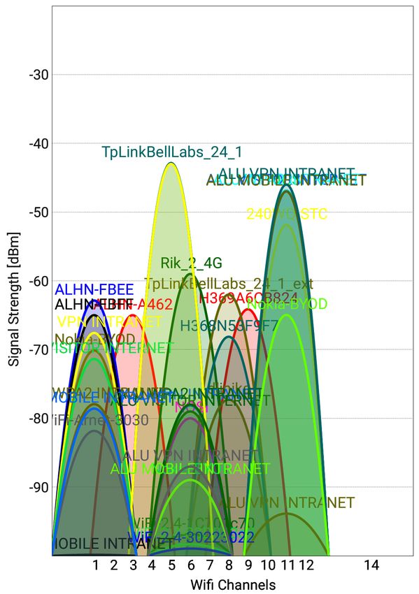
a larger scale using the simulator to address the corner            using different heuristic optimization techniques (i.e., such
     cases and unveil performance bounds in a controlled                 as genetic algorithm (GA), simulated annealing (SA), local
     environment which provides a benchmark for future self-             search (LS) and tabu search (TS) [4], [5], [8] or developing
     deployment algorithms. The resultant QoS performance                guided heuristic [6], [15]).
     is compared against that of the existing techniques to
     demonstrate the competence of the proposed framework                B. Motivation for AI
     in perceiving the neighbouring environment and reason-                 Wireless network deployment is considered as a double-
     ing the optimal deployment.                                         edged sword. A network operator or a user may deploy an EXT
A. Related Works                                                         in a position that extends the coverage of mAP, but does not
                                                                         necessarily improve QoS at the end-user location. In addition,
   The concept of self-deployment previously appeared in cel-            the EXT shares radio resources with other users connected
lular networks [5], [9], [10] and [11]. The optimal locations of         directly to the mAP. This makes a suboptimal placement of
base stations are recalculated and changed frequently accord-            extender more challenging as it increases the risk of degrading
ing to the locations of hotspots and obstacles in order to satisfy       the total system throughput [14]. Both survey-based and
capacity and coverage constraints. Wireless network self-                computer-based wireless deployments have complementary
deployment is more challenging due to shared (unlicensed)                features, yet they face the following challenges:
spectrum and non-uniform layouts creating coverage holes and
                                                                            1) Dynamics in the indoor environment: The indoor envi-
hidden node problem.
                                                                                 ronment typically experiences spatio-temporal variations
   Wireless deployment aims to find the minimal number and
                                                                                 in both demand and coverage. The spatial demand of
optimal locations of APs such that the network performance
                                                                                 users can change over the time due to utilizing services
and user QoS are maximized either manually or computer-
                                                                                 with different bandwidth or latency requirements. The
based [4]– [8]. The former refers to using a test hardware
                                                                                 coverage of deployed nodes varies due to activities of
tool to perform a site survey for the indoor environment.
                                                                                 users (e.g. mobility) and orientation of devices [7].
Experienced network engineers temporarily deploy wireless
                                                                            2) Neighboring network knowledge: A neighboring net-
transmitters (e.g. additional APs) in candidate positions to
                                                                                 work refers to another wireless system (i.e. another
measure the coverage level. Based on human experience, dif-
                                                                                 mAP-EXT pair) that is utilizing the same spectrum,
ferent locations and number of transmitters are tested until the
                                                                                 but managed by another operator. While neighboring
best coverage is achieved (e.g. no coverage holes). Although
                                                                                 network knowledge is captured by the manual deploy-
optimal coverage-based deployment can be achieved, the time
                                                                                 ment, their spatio-temporal dynamics are not. In addition
taken during the survey further increases with the size of an
                                                                                 to coverage and demand variations in neighboring net-
environment (e.g. the number and complex layout of rooms)
                                                                                 works, other network operators might deploy new APs
making the planning process prohibitively expensive.
                                                                                 or extenders or reposition existing ones within the same
   As opposed to the survey-based approach, network opera-
                                                                                 geographical region causing changes in interference and
tors adopted off-line planning software to calculate an optimal
                                                                                 contention behaviors.
deployment. In essence, the software uses path loss models,
traffic maps and building layout (e.g. number of rooms and                  The problem at hand is to find the optimal locations of
type of walls) to find the optimal location and number of                extenders associated to mAP such that the users’ demands
APs/EXTs by dividing the layout into square grids repre-                 are satisfied. The optimal extender position has to balance
senting candidate locations for APs. Different configurations            the capacity on both links, the backhaul link (i.e. between
are tested by adding and removing the APs in the grids and               mAP and EXT) and the fronthaul link (i.e. between EXT and
detect their ability to satisfy the coverage, demand and other           user). In Fig. 1, we present an isolated apartment scenario to
planning constraints. The software picks the configuration that          illustrate the drawback of coverage based approach and the
satisfies all constraints and optimizes given network metric             potential of AI-driven self-deployment proposed in this paper.
such as minimum cost or maximum throughput. Computer-                    Having mAP placed in the grid location (1,1) the following
based deployment is less expensive and more time-efficient               three scenarios are considered:
than the survey-based approach. However the optimality is                   • Single AP per apartment in Fig. 1(a-b), where the posi-
highly sensitive to the accuracy of path loss model being a                    tion is restricted to the existing wired infrastructure, re-
function of different layouts - obtaining the layout for each                  sulting in coverage holes illustrated in Fig. 1(a) with low
scenario is unfeasible. Network operators tend to follow a                     throughput values shown in Fig. 1(b), which necessitates
conservative strategy by deploying more EXTs to compensate                     deployment of an extender;
the errors in path loss model. Nevertheless, the traffic demand             • Conventional coverage-driven deployment in Fig. 1(c-d)
map might vary over time and the off-line calculated locations                 with the extender in the center of indoor area (i.e. midway
are no longer optimal.                                                         between the mAP and coverage hole). Although the
   The main challenges of existing approaches are a lack an                    overall coverage is maximized as illustrated in Fig. 1(c),
algorithm to perceive the environment and high complexity                      such approach does not improve the throughput at user
of optimization problem. These challenges are tackled by                       location as shown in Fig. 1(d)). This is due to overlooking

                                                                     2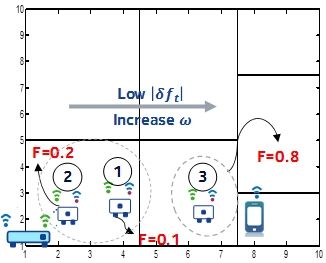
the back-haul link throughput, while only maximizing the II. N ETWORK M ODEL
front-haul link (extender-to-user). Even worse, inexperi- A. System Model
enced users will most likely place the extender closer to
The system consists of single mAP and a group of extenders
their devices, which reduces the back-haul throughput and
which are connected to mAP directly or through other exten-
consequently, limiting achievable service quality. Such
ders. The location of mAP is static and already determined,
solution is anticipated by the existing literature on EXT
while locations of extenders can be changed through time
deployment that aim to minimize the packet transmission
controlled by the proposed AI framework. We assume that a
delay and maximize the coverage [14], [16].
new location is calculated by the framework and recommended
• The proposed AI-driven self-deployment approach is
to the user by a request at t ∈ T .
adopted in Fig. 1 (e-f) to sense and learn the environment,
We note that the framework can be hosted either on mAP or
and reason the location that achieves the best compromise
in the cloud taking decisions for a whole system. The frame-
between back-haul and front-haul throughput. Hence,
work collects the sensing data (i.e network metrics) and based
improves the total throughput as shown in Fig. 1(f) while
on the current network metrics and historical data derives real-
compromising the coverage as observed by comparing the
time solutions for extender relocation. The detailed system
Fig. 1(c) and (e).
model is described by the following system variables.
1) Deployment Decision Variables: The location of each
Hence, a novel self-deployment approach needs to capture the extender is changed based on the network conditions, and we
dynamics of neighbour’s interference and contention, caused define the following variables
by variations of demand, placement of new APs or EXTs, that • δi,t equals to 1 if the extender has to be deployed at
provokes the optimality of locations. location i ∈ I after request t ∈ T ; and equals 0 otherwise
• αi,t equals to 1 if an extender has to be removed from
or deployed at location i after request t; and equals 0
10 10
otherwise. This variable is used to track the number of
1400
9 −20 9 extender repositions.
8 8 1200
7
−40
7
2) Association Variables: Each extender can be treated as a
1000
6 −60 6 station associated to other extender or mAP. Hence, we define
800
5
−80
5
600
an association variable xi,t,u which is equal to 1 if the station
4 4
3 3 400
(extender or user) at location u is connected to the extender
−100
2 2
200
at location i after request t; and equals 0 otherwise.
1 −120 1
2 4 6 8 10 2 4 6 8 10 3) Throughput Variables: The extender comprises of wire-
less connection with mAP (called backhaul link) and toward
(a) Coverage (b) Throughput
users (called fronthaul link) thus the corresponding throughput
10 10
−20 1400
variables are defined as follows:
9 9
(b)
8 8 1200 • r̂i,t denotes the estimated throughput at the back-haul of
−40
7 7 1000 extender deployed at location i after request t. This vari-
6 −60 6
5 5
800 able is obtained as modulation and coding scheme (MCS)
−80
4 4 600 index [30] having minimum difference from the maxi-
3 3
−100
400
mum achievable throughput C = B × log (1 + SN Ri,t ),
2 2
200
1 −120 1 where B denotes the channel width and SN Ri,t denotes
2 4 6 8 10 2 4 6 8 10
the signal-to-noise ratio at location i after request t
(c) Coverage (d) Throughput determined based on free-space pathloss model.
(b)
10 10 • r̄i,t denotes the actual throughput measured at the back-
−20 1400
9 9 haul of extender deployed at location i after request t.
8 8 1200
7
−40
7
Its value depends on the actual selected MCS and the
1000
6 −60 6 decisions of MAC protocol (e.g. resource allocation and
800
5
−80
5
600
clear channel assessment (CCA)) obtained by the station
4 4
3 3 400
statistics at an access point (mAP or other extender) to
−100
2 2
200
which target extender is connected. For example, either
1 −120 1
2 4 6 8 10 2 4 6 8 10 by vendor specific interface or through TR-069 protocol
(i.e. InternetGatewayDevice. LANDevice. {i}. WLAN-
(e) Coverage (f) Throughput
Configuration. {i}. AssociatedDevice. {i}. TxBitRate)
Fig. 1. Three indoor deployment scenarios where left and right figures,
respectively, denote coverage and achievable user throughput in isolated [33].
(f )
apartment, with AP placed in position (1,1). • r̂i,t,u denotes the estimated front-haul throughput of the
user at location u and connected to extender or mAP
at location i after request t. This value is generated
3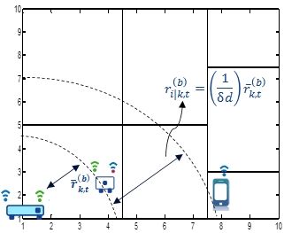
(b)                             (f )
      in the same way as r̂i,t from above. Based on r̂i,t,u ,             which necessitates conscious and fast learning by the network.
      the distance based front-haul throughput is calculated as           The problem can be mathematically formulated as follows:
        (f )   PU             (f )
      r̂i,t = u=1 xi,t,u r̂i,t,u .
        (f )                                                                                    (                                                )
  •   r̄i,t,u denotes the actual throughput measured by the user                                           X                X X
      at location u and connected to extender located at i                     minimize             max           δi,t +                  αi,t        (1)
                                                                                  α,δ               ∀t∈T
      after request t. This value depends on the actual selected                                           ∀i∈I            ∀t∈T ∀i∈I

      MCS, and the MAC decisions (e.g. resource allocation                                                                              subject to:
                                                                (b)
      and CCA) and it is calculated in the same way as r̄i,t
                                       (f )                                               C1: αi,t ≥ |δi,t−1 − δi,t |∀t ∈ T , ∀i ∈ I
      from the above. Based on r̄i,t,u , the distance based front-                            I
                                               (f )  PU      (f )                             X            (f )
      haul throughput is calculated as r̄i,t = u=1 xi,t,u r̄i,t,u ,                  C2:            δi,t r̄i,t,u ≥ Dt,u , ∀t ∈ T , ∀u ∈ U,
      where u is the user index.                                                                i=0
      ri,t denotes E2E user throughput for all users connected
                                                                                                          n             o
  •                                                                                       (f )               (f ) (b)
                                                                               C3:      r̄i,t,u ≤ δi,t min r̂i,t , r̄i,t xi,t,u , ∀t ∈ T ,
      to extender located at i after request t. This value can
                                            (b) (f )
      be measured as ri,t = min (r̄i,t , r̄i,t ) or calculated as                                                               ∀i ∈ I, ∀u ∈ U
                PU                                                                                     (b)               (b)
      ri,t =      u=1 xi,t,u ri,t,u , where ri,t,u = (T XBytes +                             C4:     r̄i,t   ≤    δi,t r̂i,t yi,t ∀t   ∈ T , ∀i ∈ I
      RXBytes) × 8/∆t, where T XBytes and RXBytes,
                                                                                             C5:     αi,t , δi,t ∈ {0, 1} ∀t ∈ T , ∀i ∈ I
      respectively, denote the total number of bytes transmitted
      and received for the user u within time interval ∆t. For            The objective function in Eq. 1 aims to minimize both the
      examples these values are available through specific ven-           deployment cost and reconfiguration costs.
      dor extensions (e.g. statistics counters InternetGateway-              The first term in the objective represents the deployment
      Device. LANDevice.{i}. WLANConfiguration.{i}. Asso-                 cost calculated by the total number of deployed extenders. The
      ciatedDevice. {i}. Stats.BytesSent and InternetGateway-             second term represents the reconfiguration cost and calculated
      Device.LANDevice. {i}. WLANConfiguration.{i}. As-                   as a function of the number of extender displacement. The first
      sociatedDevice.{i}. Stats.Bytes Received, respectively).            constraint C1 defines the reconfiguration cost as a function of
      Although the second way to obtain E2E user throughput               the difference between each two time successive deployments.
      is more accurate it’s drawback is requirement that the              Thus allows the optimizer to pick the solution that can satisfy
      user devices are always active with the transmitting and            all the time horizon demands or requires a small number of
      receiving data requests.                                            changes in the locations of deployed elements. The demand
   4) Demand Variables: The demand of every user at location              satisfaction of each user at every time instant is captured by
u after request t is denoted by Dt,u and represents the                   the constraint in C2. The set of constraints in C3-C4 are used
minimum throughput needed by the user to satisfy target QoS.              to calculate the user’s throughput (used in C2) as a function
The demand of each user can be obtained during the initial                of the actual back-haul throughput, its maximum achievable
deployment of wireless system in scope of Service Level                   value, and the MAC decisions captured by yi,t that represent
Agreement (SLA) between the user and a service provider.                  the ratio of AP’s resources devoted to extender i. The last
More advanced approach to obtain these variables would be                 constraint in C5 ensures that the two decision variables are
by using traffic prediction techniques as in [28], but this is out        binary. Unlike the plethora of Wi-Fi deployment approaches
of the scope of this paper. We assume that these variables are            that focused only on optimization techniques to solve similar
given by SLA.                                                             formulations, we focus also on how network metrics such as
                                                                          throughput can be obtained at minimal cost through learning,
                                                                          and how to leverage the previous decisions to derive future
B. Problem Formulation
                                                                          recommendations.
   As it is already said, the proposed AI framework is a                     The computational hardness property of the above defined
centralized architecture which is aiming to find the optimal              problem is provided by the following Lemma.
location of each extender in such way that each user demand                  Lemma 1. Dynamic Location optimization in WMNs pos-
is satisfied at each time instant. Based on that the problem is           sess the non-deterministic polynomial-time hardness (NP-
finding the optimal location(s) of extender with minimal cost.            hard) property.
Unlike existing approaches, the framework does not have any                  The proof of Lemma is given in Appendix A.
prior knowledge about the network. As such, the layout of the                Hence, below we present a case based heuristic algorithm
building or wall losses are not adopted. This is in addition to           with semi-supervised learning to achieve a near-optimal de-
the unavailability of neighbour information such as locations,            ployment of extenders.
channel configurations and traffic load. As such, the network
will notify the user to change the location of extender to 1)                           III. AI-D RIVEN S ELF -D EPLOYMENT
learn the environment, and 2) improve his QoS level. It is                  A key component of self-deployment is the autonomy, in
therefore of paramount importance to minimize the number                  which the network can optimize the extender location without
of requests to the user, i.e. ask the user to move the extender,          manual troubleshooting or instructions from operator help

                                                                      4
desk. To that end, AI is adopted and models the network as two throughput, ri,t,u and the requested user demand, Dt,u , i.e.
main elements: 1) environment and 2) intelligent agent. The ri,t,u
former refers to wireless systems and other objects including fi,t,u = (2)
Dt,u
neighboring networks, either coordinated or uncoordinated,
indoor obstacles and backbone network, among others. The if fi,t,u is higher than 1, it is set to 1. The fitness value
intelligent agent perceives the environment through a sequence represents the QoS satisfaction degree.
of sensing, reasoning and acting in order to build its own While the system consistently senses the environment and
knowledge and use it in future actions. Thus, good actions, receives measurements s, the CBR undergoes the following
e.g. satisfies the QoS levels, can be reused directly in future four main stages [19], [20]:
when similar network conditions are sensed, while bad actions, 1) Retrieve the most relevant case, in the knowledge base,
e.g. created coverage holes, will be used to refine the searching to the currently sensed information
strategy of the agent [17]. 2) Reuse the retrieved case or relative experience to solve
The AI can be implemented in different forms such as rule the sensed problem
based system (RBS), ontology based system (OBS) and CBR, 3) Revise the knowledge base by updating the actions or
among others [18]. The RBS comprises a set of rules with fitness values of the stored cases
predefined actions created by experts in the network domain. 4) Retain the learned experience (e.g. new case) in the
Similarly, OBS applies logic based reasoning for the domain knowledge base to be used in the future
attributes. This logic involves a set of 1) classes: that define a In the following subsections we demonstrate the implemen-
set of objects in the modeled domain; 2) instances: individuals tation of every stage using the six main blocks (Step 1-6)
of each class; 3) attributes: properties of each object; and 4) in Fig. 2. The main stages of the prosposed framework are
relations: to define relationships between different objects and summarized in Algorithm 1 , as well. Unlike the agent-based
attributes. approach in [21], where fully coordinated single-hop Wi-
Unlike CBR, both RBS and OBS require explicit domain Fi network and the availability of neighbouring environment
knowledge to define the relations between rules and actions or information are assumed beforehand, our agent continuously
objects. While CBR adopts the system memory to build the senses and learns the environment to gain experience and
knowledge using previous actions and capture their impact on generate new actions. The agent enables network intelligence
the network. Thus, CBR is well suited for wireless network to capture the impact of dynamic neighbouring networks and
with none fully observable environment (due to dynamic and floor layout while calculating optimal extender’s location.
uncoordinated deployment, unknown layout plan) and complex
B. Sensing and Perception
operations to be controlled by human-based rules. However,
one of the key issues of CBR are propagation errors through The first step is sensing the environment which involves
cases. To overcome this issue CBR systems are often used in collecting the measurements from the user devices, mAP and
combination with learning such as reinforcement learning [31] extenders through TR-98/181 protocol for remote manage-
- [32]. The reinforcement learning also benefits from CBR ment [33] or other programmable application interfaces. The
system which significantly speeds up learning of unknown collected information contains radio-interface level statistics
environment and improves its efficiency. Having said that, here (e.g used channel width, channel indices, noise level etc.)
we consider CBR in combination with reinforcement learning, and user-device level statistics (e.g. RSSI, TxBitRate, RxBi-
where to each problem and solution we assigned the reward tRate, counters for sent and received bytes etc.). The sensing
value which is determined as fitness value. stage collects the data with a certain period τ in seconds.
The perception stage translates the sensed information into
A. Proposed Framework Overview performance indicators (i.e. system variables) that identify the
We adopt a CBR AI framework shown in Fig. 2. The network state. This information will allow the agent to perceive
CBR relies fundamentally on a KB that stores previous cases the environment, to learn and estimate throughput values for
experienced by the self-deployment system, where each case not visited locations and assess the level of user satisfaction.
is a triplet of problem (P), action (A) and fitness (F). The The performance indicators are calculated for each user
problem refers to a set of measurements that describes the (user device or extender) based on two successive sensing
current situation of the network where a user is unsatisfied. samples. These indicators include:
The problem is a vector that contains both the locations and • Average RSSI - The received signal strength indicator
demands of users associated to the extender and the location (RSSI) at user location u from sink node (extender)
of AP. For each stored problem, an action can be performed, placed at location i after request t, RSSI i,t,u presents
where action refers to a new position of the extender. After the a measured received signal strength in dBm of bea-
action is applied in the environment (i.e. user repositions the con frames received on the channel (i.e. defined as
extender), the fitness of this action is calculated based on the dot11BeaconRssi [34]). RSSI is usually measured during
degree of user demand satisfaction. Accordingly, we denote the the reception of the physical (PHY) preamble and its
fitness for user at location u associated to extender at location value is forwarded to medium access control (MAC) layer
i after request t, fi,t,u as a ratio between the achievable user in the RXVECTOR [34]. Beacon’s RSSI may be averaged
5Update A
Knowledge Step 6
Base [A,F] Optimization
Update F
[c*, k*,a*]
C Step 5
Step 4
Decision
Reasoning
Problem (P) Action (A) Fitness (F) Making
[AP Loc, User Loc, D] [Ext Loc] [Rb, Rf, Q] a*
Step 3
k =[loc, D, -, -]
Learning
[{1,1}, {5,5}, 100] (x1,y1) [50,10, 0.7] Environment
k= [loc, D, R, -]
[{1,1}, {2,5}, 100] (x2,y2) [90,90,0.9]
[{1,1}, {8,9}, 100] (x3,y3) [10,10,0.1] s=[RSSI, RTT, Bytes]
Step 2 Step 1
Perception Sensing
Fig. 2. AI-CBR Framework for Self-Deployment.
1 © 2016 Nokia
over time using a vendor specific smoothing function. relevant case c∗ is calculated as follows:
In case that the beacon frame is received by means of
s X
multiple receive chains, the RSSI is averaged in linear k∗ = argmin (pk,j − p̄j )2 (3)
domain over all chains. The valid range of RSSI values k∈K
j∈J
is -100 to 40 dBm [34].
• Average Noise Level can be obtained through the Noise where K is the set of stored cases in the knowledge base and
Histogram request/report pair which returns a power his- pk,j is the j th entry of the k th stored problem.
togram measurement of non-IEEE 802.11 noise power by Besides deterministic reasoning other approaches based on
sampling the channel when virtual carrier sense indicates probabilistic reasoning (belief network) may be used, but that
idle and the STA is neither transmitting nor receiving is out of the scope of this work.
a frame. This value is denoted as average noise plus D. Decision Making
interference power indicator (ANIPI) and its value is
contained in Noise histogram report [34]. The decision making step has to determine whether the
• E2E User Throughput is calculated by using transmitted action of the most matching case can be reused and pushed
and received bytes counter values such it is described in to the user or a new action has to be recalculated.
section II-A. The decision-making step will check both the calculated
matching factor given by Euclidean distance in Eq. 3 and the
The output of the sensing and perception stage will be used fitness value given by Eq. 2 of the retrieved case. For instance,
to trigger each of the following stages as discussed below. the decision making returns true, and applies the action, if both
the matching factor is below a maximum threshold, denoted
C. Reasoning by M̂ while the fitness value f ∗ is above a minimal level F̂ . If
this condition is not met, then either no matching cases exist
The perception output will allow the framework to detect in the knowledge base and thus a new case must be retained,
if the network is experiencing problems such as unsatisfied or the best matching case has a suboptimal action that must
user. As an example, when the measured throughput by the be revised.
perception is lower than the user’s demand (i.e. f < 1), the
framework will trigger the reasoning module to compare the E. Optimization
current situation (i.e. perception output) with the previously The optimization step aims to calculate a new action that
experienced situations (i.e. problem). Reasoning is performed will be retained in the knowledge base. In principle, existing
to retrieve the most relevant case from the knowledge base and actions in the knowledge base will be used to guide the search
reuse the corresponding action to solve the current problem. direction. Two main strategies are followed while creating the
In particular, the current perceived problem p̄ is compared to new action: exploitation and exploration. The former stands
all the stored problems P in the knowledge base to calculate a for greedily optimizing the network metrics within a limited
matching factor. The action and fitness of the most matching search space that is assumed to be promising. On the contrary,
case, denoted by a∗ and f ∗ (i.e. corresponding to a single raw the exploration tries to discover new search spaces that can
in KB), are checked afterwards in the decision making step lead to more promising solutions than the currently exploited
to determine if they can be reused. The index k ∗ of the most solution set. The exploration and exploitation strategy [35],
6[36], [37] is decided by policy which is described below. The ω that control the degree of exploration of the logarithmic
policy is controlled by an exploration factor whose value is function. Where at low values such as ω = 0.1 the near
learnt and adjusted with each new action. Although, there are locations are assigned very high values, which provides limited
a lot of undirected exploration techniques proposed in litera- exploration, i.e. exploitation. On the contrary, high values
ture (such as Random Exploration, Semi-Uniform Distributed such as ω = 1 provide steeper decay with the distance, and
Exploration and Boltzmann Distributed Exploration) which thus assigns higher fitness to the far locations, not visited
randomly explore the environment without consideration the before, resulting in wider-scale exploration. The principle of
previous history of the learning process, here we apply a exploration factor is illustrated in Fig. 3(c). The minimum
directed exploration. It is worth to stress once more, the operator in the objective function selects only one entry from
repositioning of extender involves the user and has a high the knowledge base to evaluate the exploration fitness of the
cost regarding service disruption due to device re-association candidate locations.
time which should be minimized. Hence, with this in mind, 3) Action Generation: The final action comprises one loca-
the random exploration deems unacceptable in this case. tion that balances both the exploitation and exploration fitness
1) Objective: The first problem to be optimized is the user values. Herein, we adopt the multiplication of both values to
end-to-end throughput at user devices. While such throughput represent the overall fitness as given by
depends on both the back-haul and front-haul throughput (
values at the extender, a minimum operator is applied as maximize {FR × FE }
δ (6)
depicted in the below formulation as follows: subject to: C1, C2
n o
(b) (f )
Thus, solutions that are far from those previously visited and
P
maximize
FR = ∀i∈I δi,t min (r̂i,t , r̂i,t )
δ
expected to have high throughput at the end user will have the
subject to: (4) maximum fitness.
PI
C1: i δi,t ≤ N ; ∀t ∈ T
C2: δi,t ∈ {0, 1} ; ∀t ∈ T , ∀i ∈ I F. Learning
The last stage, learning, involves revising and retaining the
The objective function in Eq. 4 represents the end-user entries in the knowledge base, and adapting the threshold
achievable throughput by each deployed extender after request values and parameters in the other stages based on the mea-
t. It has to be noted that the optimization step adopts estimated surements. Per each iteration, the learning stage updates the
values whose accuracies are improved by the learning stage fitness value as in (2) for a certain user at location u, and asso-
discussed later. ciated to extender at location i. While autonomous operation
The constraint C2 defines the extender location as a binary of the AI framework is paramount, yet the user is involved
decision variable, while constraint C1 bounds the number of by repositioning the extenders, semi-supervised learning is
selected locations to the N deployed extenders. adopted to learn: 1) system variables (i.e. throughput variables)
2) Exploration and Exploitation Policy: The trade-off be- and 2) exploration factor.
tween exploration and exploitation is very challenging. The Supervised learning techniques are not applicable due to
exploration strategy enables the optimizer to try different lack of full knowledge about the environment (i.e. floor plan
regions where throughput is assumed to be low (e.g. far rooms and neighbouring traffic). Thus, in our case, the learning stage
from the AP but also far from the hidden node neighbor) in is designed to improve the accuracy of system variables by
order to maximize the acquired knowledge. This exploration leveraging previously learnt values.
is achieved by assigning low fitness values to the previously 1) Throughput Values: The throughput estimation is very
visited locations, or the positions in their proximity, and vice challenging due to: 1) the dependency of the front-haul on
verse. On the other hand, the exploitation limits the optimizer the back-haul value, and 2) the existence of neighbours that
to search in a small region (e.g. in the same room) while can cause hidden nodes. The first necessitates learning the
no throughput improvements are observed at the user device. front-haul values only when the back-haul is maximized, while
To that end, the optimizer leverages the saved actions in the the latter makes the distance-based throughput estimation
knowledge base (i.e. previous visited locations) and calculates inaccurate as more interference can be encountered at while
their distance to the candidate locations as follows: placing the extender in the direction of interfering neighbour.
(
maximize FE = min {δi,t (log10 ζk,i )ω } In essence, the learning stage has to utilize the previously
δ ∀k∈K (5) measured throughput values at different locations in order to
subject to: C1 - C2 improve the estimation in other undiscovered locations. After
In the above expression, ζk,i depicts the distance between the each request t, the set of available measurements from the
candidate location i and each of the saved locations k ∈ K previous k ∈ K actions is used as labelled data to estimate
in the knowledge base. The logarithmic function is selected the throughput in other not visited locations.
to avoid very far locations from the previously visited. Thus, • Learned Backhaul Throughput: Semi-Supervised support
provide a gradual exploration that does not overestimate such vector machines (S3VM) [24] are therefore used to up-
(b)
far locations. In this, work, we adopt an exploration factor date the estimated back-haul throughput r̂i,t at location
7i as a function of: distance based estimated throughput of similar fitness values obtained by the generated actions, and
at the current and previously visited locations, and the vice versa. This strategy is depicted as follows:
measured value of the latter as given by (
ωt = 12 (ωt−1 + δωt ) ∀t ∈ T (a)
(b) (b) (b) (b) (10)
r̂i,t = F(r̂i,t , r̂k,t , r̄k,t ) ∀k ∈ K, ∀i ∈ I. (7) δωt = 2 − e|δF | (b)
Each of the measured throughput values is used to define In Eq. 10(a), the exploration factor is updated after each
two regions: between location k and the AP (i.e. Region request t using the previous value and the step variable δωt .
1), and between the location k and the connected users The latter is calculated based on the difference in the fitness
(i.e. Region 2) as illustrated in Fig. 3(b). According to values of the last two actions. The exponential function in
that, F has the following definition Eq. 10(b) results in negative values if the absolute fitness
difference |δF | is high which will decrease the value of ωt in
Eq. 10(a) to limit the exploration, i.e search in limited region.
(
(b)
(b) r̄k,t i ∈ Region 1
r̂i,t = 1 (b) On the other hand, low |δF | results in higher ω that maximizes
δd × r̄k,t ∀k ∈ K, ∀i ∈ I i ∈ Region 2,
the exploration as illustrated in Fig. 3(c). It has to be noted
(8) that δF ∈ [−1, 1] and thus the calculated value in Eq. 10(a)
is normalized.
where δd is the difference in the distance between lo-
cations i and k. While the throughput in the Region
1 remains the same as the measured value, the values
decreases gradually in the Region 2. As more measure-
ments become available, the regions are redefined to
obtain non-overlapping boundaries using the S3VM in
[24]. The distance based throughput is used to classify the
location in one of the throughput regions. Initial values
of estimated throughput variables are calculated as it is
mentioned in Section II. (a) Learning backhaul (b) Learning backhaul through-
• Learned Front-haul Throughput: Follows the same proce- throughput: illustration of put: region definition and estima-
dure as the back-haul except that the gradually decreasing back-haul throughput in Eq. 7 tion in Eq. 10.
function is applied in the former region (i.e. between AP
and extender). The main challenge is to decouple the
impact of back-haul on the front-haul throughput calcu-
lation. As such, a region is defined in which the network
guarantees that the reported front-haul throughput is only
due to the channel conditions between the extender and
the user, and not due to poor back-haul link. As such,
this region is defined as the area between the extender and
user locations in which the back-haul throughput satisfies (c) Principle of exploration step in (d) The adjustement of Explo-
Eq. 5 ration Factor
the demand or surpasses the total front-haul. Thus, the
(f ) Fig. 3. Illustration of different learning principles.
updated estimated front-haul throughput r̂i,t at location
i is a function of: 1) distance based estimated throughput
at the current and previously visited locations, and 2) the IV. P ERFORMANCE E VALUATION
measured value of the latter as given by
A. Experimental Setup
(f ) (f ) (f ) (f )
r̂i,t = F(r̂i,t , r̂k,t , r̄k,t ) ∀k ∈ K, ∀i ∈ I. (9) 1) Testbed Environment: The experimental testbed consists
of AI framework, a single wired-backhaul AP, i.e. mAP,
where F is defined in Eq. 8, while Region 1 is defined as a single extender (EXT) and an end-user device which is
a region between location i and location k, and Region connected to mAP through EXT. AI framework logic is
2 is defined as region between location k and location n, implemented in MATLAB and hosted in the cloud. AI engine
where is n > k. has a secure connection to mAP, which is used to collect
2) Exploration Factor: The exploration factor is a key of network parameters and to push change-location notifications
policy to control exploitation and exploration and it controls to the end users via embedded speaker. For mAP we consider
how far the extender should be placed from the previously dual-band TP-Link AC1750 AP, whereas EXT is a single-
visited locations that are deemed suboptimal. The exploration band GL-MT300A operating on 2.4 GHz. EXT is configured
factor ω is thus adapted based on the reported fitness values as a simple repeater of the signal received from mAP and the
to guarantee visiting spatially separated regions. As such, the signal received from the user devices associated to itself. In
value of ω has to be increased, thus higher exploration, in case other words, EXT operates as a station connected to mAP at
8߱ ൌ ሼʹǤͶǡ ͷሽ
ߜʹǡ߱
ߜͳǡ߱
ߜ͵ǡ߱
17 m 1 2 3
߱ ൌ ሼʹǤͶǡ ͷሽ ߙ ሺܧሻ݂ǡ߱
Step 6 ߙ ሺܧሻ ܾǡ߱
User
Optimization
ߜʹǡ߱
ߜͳǡ߱
ߜ͵ǡ߱
Knowledge Step 5
Step 4
Base Decision
Reasoning
Making ߱ ൌ ሼʹǤͶǡ ͷሽ ߙ ሺܧሻ݂ǡ߱
ߙ ሺܧሻ ܾǡ߱
Step 3 ߜʹǡ߱ ߱ ൌ ሼʹǤͶǡ ͷሽ
ߜͳǡ߱
Learning ߜ͵ǡ߱
߱ ൌ ሼʹǤͶǡ ͷሽ
ߜʹǡ߱ 1
ߜͳǡ߱ ߙ ሺܧሻ݂ǡ߱
Step 2 ߜ͵ǡ߱
ߜʹǡ߱ ߙ ሺܧሻ ܾǡ߱
22 m
Step 1 ߜͳǡ߱
Perception Sensing ߜ͵ǡ߱
Extender 3 ߙ ሺܧሻ݂ǡ߱
ߙ ሺܧሻ ܾǡ߱
AI ߙ ሺܧሻ݂ǡ߱
߱ ൌ ሼʹǤͶǡ ͷሽ ߱ ൌ ሼʹǤͶǡ ͷሽ Framework ߙ ሺܧሻ ܾǡ߱ 2 Extender
߱ ൌ ሼʹǤͶǡ ͷሽ
Extender
ߜʹǡ߱
LEDE, LEDE, ߜʹǡ߱
ߜͳǡ߱
ߜ͵ǡ߱ ߜʹǡ߱
ߜͳǡ߱
ߜ͵ǡ߱
Sensing ߜͳǡ߱ Sensing
Shell Scripts ߜ͵ǡ߱ Shell Scripts
SSH
ሺܧሻ ߙ ሺܧሻ݂ǡ߱
2.4 2.4 ߙ ݂ǡ߱ ߙ ሺܧሻ ܾǡ߱
ߙ ሺܧሻGHz
ܾǡ߱ GHz ߙ ሺܧሻ݂ǡ߱
Raw network data APAccess point
E
ߙ ሺܧሻ ܾǡ߱
EXT Power
Extender
mAP
neighborAP 1 Access point neighborAP N
SSH
Bank STA
neighborAP 2
Environment New EXT location (a) Environment (b) Throughput Measurements
Fig. 5. Testbed results for coverage problem (midway initial position).
Fig. 4. AI Testbed with off-the-shelf devices.
Algorithm 1: Dynamic Location Optimization
Input : Knowledge Base (Cases, Fitness Values, User
Demands, Perception data);
Output : Action a∗ ;
1 Define: Max. matching threshold: M̂ , min. fitness threshold: F̂ ,
max. number of repositioning actions N ;
2 for each extender i in the network do
3 Update estimated backhaul throughputs using Eq. 8;
4 for u ∈ U associated to extender i do
5 Update estimated fronthaul throughputs using Eq. 9;
6 Update fitness value for user at location u associated to
extender i using Eq. 2;
7 /* Check if the user demand is satisfied */
8 if ri,t,u < Dt,u then
9 /*Reasoning*/
10 Find the best matching case c∗ := (a∗ , f ∗ ) in KB (a) mAP location (b) EXT at location 1
using Eq. 3;
11 /*Decision Making */ Fig. 6. 2.4 GHz wireless spectrum at the locations of mAP and EXT in
12 if k∗ < M̂ and f ∗ > F̂ then Fig. 5(a) at location 1 (similar density of neighbouring networks is observed
13 apply action a∗ at locations 2 and 3 with distance of 2 and 4 meters, respectively, from location
1.
14 end
15 else
16 /*Optimization*/
17 Adjust exploration factor by Eq. 10 and Fig. 5(a) .
generate new action a0 by Eq. 6; 2) Coverage Problem: We applied the experimental testbed
18 if total number of extender repositioning < N
19 apply action a0
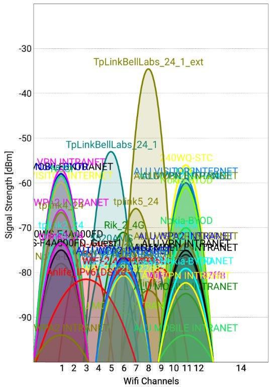
in an enterprise scenario as shown in Fig. 5(a). The environ-
20 end ment employs a large number of uncoordinated neighboring
21 end Wi-Fi APs as illustrated by the scan of the spectrum in Fig. 6.
22 end Due to different received power levels of neighboring APs,
23 end exposed and hidden nodes are experienced by the coordinated
24 end
network on which the AI framework is tested. With such an
ultra dense scenario, we manually set the operating channel
after manual tuning to minimize contention at the AP. Other
the side of backhaul link and as an access point operating in parameters are summarized in Table I. The extender is initially
infrastructure mode on the side of fronthaul link. Since EXT placed in the mid-way between the AP and user device.
is battery powered (connected to a power bank via USB), its The throughput measurements are reported in Fig. 5(b) for
location is not restricted to the locations where electric plugs the three locations of extender where the location index is
are available. We equipped EXT with usb-to-audio adapter shown in circles in Fig. 5. The second and third locations are
and a speaker device, in order to be able to produce audible successively calculated by the proposed AI framework and
change-location notifications to the end users. The indoor resulted in an end-to-end throughput improvement of 300%
localization information is assumed available. We installed at the last location compared to the initial mid-way based
LEDE images [25] on both mAP and EXT and by means of one. In particular, The AI-framework gradually improves the
shell scripts, periodical network parameters are reported to the backhaul throughput by placing the extender closer to the AP.
cloud hosting the AI framework. mAP and EXT are deployed The third location, i.e. the optimal one, compensated the high
in an uncoordinated environment whose layout is shown in partition attenuation factor of the glass walls between the mAP
9߱ ൌ ሼʹǤͶǡ ͷሽ ߱ ൌ ሼʹǤͶǡ ͷሽ
ߜʹǡ߱ ߜʹǡ߱
ߜͳǡ߱ ߜͳǡ߱
ߜ͵ǡ߱ ߜ͵ǡ߱
߱ ൌ ሼʹǤͶǡ ͷሽ 17 m 17 m
߱ ൌ ሼʹǤͶǡ ͷሽ ߙ ሺܧሻ݂ǡ߱ ߱ ൌ ሼʹǤͶǡ ͷሽ ߙ ሺܧሻ݂ǡ߱
ߙ ሺܧሻ ܾǡ߱ 15 ߙ ሺܧሻ ܾǡ߱
ߜʹǡ߱ ߱ ൌ ሼʹǤͶǡ ͷሽ
User User
ߜͳǡ߱ 1
ߜ͵ǡ߱ ߱ ൌ ሼʹǤͶǡ ͷሽ
ߜʹǡ߱ ߜʹǡ߱
ߜͳǡ߱ ߜͳǡ߱
ߜʹǡ߱ ߜ ߜ͵ǡ߱ 2 3
ߜͳǡ߱ ߙ ሺܧሻ݂ǡ߱ ͵ǡ߱ 4
Measured Throughput [Mbps]
ߜʹǡ߱ ߜ
ሺܧሻ ͵ǡ߱
ߜͳǡ߱
ߜ͵ǡ߱ߙ ܾǡ߱ 1 1 2 3 4 5 ߱ ൌ ሼʹǤͶǡ ͷሽ
ߙ ሺܧሻ݂ǡ߱ ߙ ሺܧሻ݂ǡ߱
ߙ ሺܧሻ݂ǡ߱
ሺܧሻ 5
ߙ ሺܧሻ ܾǡ߱
Extender
ߙ ሺܧሻ݂ǡ߱ ߙ ܾǡ߱ ߙ ሺܧሻ ܾǡ߱
ߜʹǡ߱
ߙ ሺܧሻ
߱ ൌ ሼʹǤͶǡܾǡ߱
ͷሽ ߱ ൌ ሼʹǤͶǡ ͷሽ
Extender
10 ߜͳǡ߱
ߜ͵ǡ߱ ߱ ൌ ሼʹǤͶǡ ͷሽ
߱ ൌ ሼʹǤͶǡ ͷሽ
2
Extender ߱ ൌ ሼʹǤͶǡ ͷሽ߱ ൌ ሼʹǤͶǡ ͷሽ
3 Hidden
ߜʹǡ߱ ߜʹǡ߱ ߜʹǡ߱ ߙ ሺܧሻ݂ǡ߱
ߜͳǡ߱ ߜʹǡ߱ ߜͳǡ߱ ߜͳǡ߱
ߙ ሺܧሻ
ߜ͵ǡ߱ ߜͳǡ߱ ܾǡ߱ ߜ͵ǡ߱ ߜ͵ǡ߱ Nodes
ߜ͵ǡ߱ ߜʹǡ߱ ߜ ߜʹǡ߱
22 m
22 m
ߜͳǡ߱ ͳǡ߱
1
ߜ͵ǡ߱ ߜ͵ǡ߱ Extender
ሺܧሻ
ߙ ሺܧሻ݂ǡ߱ ߙ ሺܧሻ݂ǡ߱ 4 ߙ5 ݂ǡ߱ ߙ ሺܧሻ݂ǡ߱
ߙ ሺܧሻ ܾǡ߱ ߙ ሺܧሻ ܾǡ߱ ߙ ሺܧሻ ܾǡ߱ ሺܧሻߙ ሺܧሻ ܾǡ߱ ሺܧሻ
ߙ ݂ǡ߱ ߙ ݂ǡ߱
4 5 ߙ ሺܧሻ ܾǡ߱ ߙ ሺܧሻ ܾǡ߱
5 Extender Extender
Extender Extender ߱ ൌ ሼʹǤͶǡ ͷሽ ߱ ൌ ሼʹǤͶǡ ͷሽ
Extender Extender
2 3
ߜʹǡ߱ ߜʹǡ߱
ߜͳǡ߱ ߜͳǡ߱
ߜ͵ǡ߱ ߜ͵ǡ߱
ߙ ሺܧሻ݂ǡ߱ ߙ ሺܧሻ݂ǡ߱
ߙ ሺܧሻ ܾǡ߱ 0 ߙ ሺܧሻ ܾǡ߱
APAccess point 0 50 100 150 200 250 APAccess point
Time [dt=25 s]
(a) Environment (b) Throughput Measurements (a) Environment (b) Throughput Measurements
Fig. 7. Testbed results for coverage problem (random initial position). Fig. 8. Testbed results for interference scenario with hidden node problem.
and EXT by minimizing the length of backhaul link. This the user satisfaction. Herein, the QoE value is calculated by
placement leverages the open space between the user device Mean Opinion Score (MOS) according to the model in [26],
and EXT, and thus the fronthaul throughput is not deteriorated where MOS varies between 1 and 5 corresponding to very
by moving the extender away from the user. poor and excellent service, respectively. In case of suboptimal
We repeated such coverage problem but with a different placement of extender such as mid-way location (i.e. location
initial location in order to assess the convergence of the AI 1) as in Fig. 7(a), the user watched a 2 minutes video in a
approach as depicted in Fig. 7(a). In this case, more locations duration of 3.6 minutes. These stops are attributed to the buffer
were recommended before the final optimal location is reached underrun at the user device since the delivered throughput is
as shown in Fig. 7(b). Thus, the cost of learning is said to be not high enough to transmit the high quality video content
higher, equals to 3, than the previous scenario whose cost on time. Thus, this stop duration of 1.6 minutes resulted in a
of learning was 1. The intermediate locations 2 and 3 in MOS around 1 which is not acceptable by end-users. On the
Fig. 7(a) demonstrate the exploitation phase where the region contrary, optimizing the location of extender results in zero
surrounding the initial suboptimal location is searched first. stops and thus the maximum MOS was achieved.
However, recommended locations did not result in significant
throughput improvements as show in Fig. 7(b). Thus, the algo- B. Simulation Setup
rithm attempted to explore the environment and recommended 1) ns-3 Environment: To complement experimental results
locations 4 and 5 that are farther from the last recommended with single-band extender and single user setup, we evaluate
locations. the proposed method using the Wi-Fi IEEE 802.11ac com-
3) Interference (Hidden Node) Problem: Beside the exist- pliant simulator ns-3. The extender is modeled as a node
ing unmanaged neighboring networks, an interfering network that implements two Wi-Fi interfaces, one working in ad-
(i.e. AP, extender and user device) is deployed close to the hoc mode, to communicate with the AP nodes, while the
managed user device and operate at the same channel. The other interface is operating in an infrastructure mode to act
location of such interfering AP is chosen such that it acts as an AP for the user station (STA). The two interfaces are
as a hidden node to the managed AP and create excessive operating on two different radios (i.e. dual-radio) both on the
interference at the BH of the managed extender as shown 5 GHz band. All the simulation parameters and values are
in Fig. 8(a). To demonstrate the worst case interference, the summarized in Table II. The maximum achievable gains of
interfering network is working in a saturated traffic mode and the proposed method are computed by adopting exhaustive
hence occupying the shared medium all the time. Such hidden search in solving the above presented optimization problem.
node scenario resulted in very low throughput values in the In this section, we further resort to computer simulation to get
initial location with a service outage 40% of the collected insights and investigate the effectiveness of AI framework in
measurements as depicted in Fig. 8(b). This is in addition more complex deployments.
to increasing the cost of learning to 2 although the same We compare the proposed framework, referred to as AI-
initial location as the first scenario was adopted. Comparing Driven CBR, with (i) the coverage maximization and delay
the throughput of the final optimal locations, i.e. 4, with the minimization approaches in [14], referred to as Coverage
initial mid-way location, i.e. 1, the former resulted in more Max., and (ii) the AP only scenario without extenders. This
than 11 times throughput improvements without any service is in addition to reporting results for the AP only scenario
outages. to illustrate the impact of creating multi-hope networks, due
4) User Experience: In the above experiments, the user to an extender, on the network performance. The proposed
was watching a Full High Definition (FHD) 2K YouTube framework will be referred to as AI-Driven CBR. The number
video while connected to the extender. The user’s quality of of reconfiguration requests to reposition the extender is set to 5
experience (QoE) can be typically measured as a function of to minimize the burden. Results are reported for 50 simulation
duration of video stops which is a critical parameter reflecting drops where the locations of users are randomly changed. The
10߱ ൌ ሼʹǤͶǡ ͷሽ
TABLE I
S UMMARY OF PARAMETERS FOR E XPERIMENT
Managed ߜʹǡ߱ Unmanaged
ߜͳǡ߱
ߜ͵ǡ߱
Parameter Value
Transmit power (AP and extender) 20 dBm ߱ ൌ ሼʹǤͶǡ ͷሽ
Bandwidth 20 MHz ߱ ൌ ሼʹǤͶǡ ͷሽ ߙ ሺܧሻ݂ǡ߱
Frequency Band 2.4 GHz ߙ ሺܧሻ ܾǡ߱߱ ൌ ሼʹǤͶǡ ͷሽ
YouTube Video Quality 2K ߜʹǡ߱
Transmission Rate Fixed: MCS 5 ߜͳǡ߱ ߜ
ߜ͵ǡ߱ ߜʹǡ߱ ߜ
Number of radios in extender 1 ߱ߜൌ
ͳǡ߱ሼʹǤͶǡ
ߜͳǡ߱ͷሽ ʹǡ߱ ߱ ൌ ሼʹǤͶǡߜͷሽ
ͳǡ߱
ߜ͵ǡ߱ ߜ͵ǡ߱
TABLE II ߙ ሺܧሻ݂ǡ߱
Hidden Nodes
ߙ ሺܧሻߜܾǡ߱ ߜʹǡ߱ ߙ ሺܧሻ݂ǡ߱
S UMMARY OF S IMULATION PARAMETERS ߜͳǡ߱ ʹǡ߱ ߜͳǡ߱ ߙ ሺܧሻ݂ǡ߱
ߜ͵ǡ߱ Extender ߙ ሺܧሻ ܾǡ߱
ߙ ሺܧሻ ܾǡ߱ ߜ͵ǡ߱
Parameter Value
ߜʹǡ߱
Transmit power (AP and extender) 20 dBm Hidden Nodes
ߙ ሺܧሻ݂ǡ߱ Extender ߜͳǡ߱
Bandwidth 80 MHz ߙ ሺܧሻ ܾǡ߱ ሺܧሻ
ߙ ܾǡ߱
Frequency Band 5 GHz
Demand {100, 150} Mbps AP AP
Path Loss Model IEEE 802.11ax
Wall Loss 10 dB 1 © 2016 Nokia
Receiver Sensitivity −83 dBm (a) 2 apartments scenario
STA Locations U [0, 10]
Rate Adaptation Minstrel
Number of radios in extender 2
߱ ൌ ሼʹǤͶǡ ͷሽ
߱ ൌ ሼʹǤͶǡ ͷሽ ߜʹǡ߱
valuation metrics is summarized below: ߜͳǡ߱
ߜ͵ǡ߱
• Average Throughput: The first metric adopted in this ߱ ൌ ሼʹǤͶǡ ͷሽ ߙ ሺܧሻ݂ǡ߱
ߜʹǡ߱ ߱ ൌ ሼʹǤͶǡ ͷሽ
evaluation is the average throughput among all theߜͳǡ߱users ߙ ሺܧሻ ܾǡ߱
ߜ͵ǡ߱
served by the same AP, either directly or through an ߜʹǡ߱ ߜʹǡ߱
ߜͳǡ߱ ߜͳǡ߱
ߜ͵ǡ߱ ߜ͵ǡ߱
extender. Thus, illustrates the ability of self-deployment ߙ ሺܧሻ݂ǡ߱ 20
to maximize the resource utilization in the network. ߙ ሺܧሻ ܾǡ߱
ሺܧሻ ߙ ሺܧሻ݂ǡ߱
ߙߙ
ሺܧሻ ݂ǡ߱
• Fairness Index: The second metric is the throughput fair- Extenderߙ ሺܧሻ
ܾǡ߱
ܾǡ߱
ness calculated using Jain’s fairness index [27]. This rep- Access point
resents the ability of self-deployment scheme to achieve
a uniform QoS satisfaction among the users. 62 m
• Service Outage: This metric refers to the percentage of
scenarios when the users receive zero throughput. As (b) 1 Floor, 10 apartments (1STA Each) scenario
such, represents the risk of having throughput holes in
the environment. Fig. 9. Example of simulated uncoordinated Wi-Fi indoor deployment.
2) Results: We simulate two isolated scenarios in which 1
apartment is considered without neighbors, and two uncoordi-
nated scenarios with unmanaged neighboring apartments. The in 10% service outages, with 79 Mbps average throughput and
apartment is a square with side length of 10 m and comprises 0.76 fairness index.
6 rooms as illustrated in Fig. 9. The above improvements demonstrate that the AI self-
Isolated Scenario: This scenario corresponds to simulating deployment is capable of 1) learning the throughput values
the coverage problem in an interference free environment, without the need of modeling the walls, 2) reach the position
where the main source of throughput degradation is the poor that balances both back-haul and front-haul throughput values,
RSSI. In Fig. 10(a), the distribution of the throughput values and 3) remove the service outages and achieve uniform QoS
by the three approaches is shown for the users connected to across the users. This is unlike the coverage maximization ap-
the extender which located far from the AP. While both the proach that typically suffered from poor back-haul throughput
coverage maximization and AI self-deployment approaches and greedy placement that maximizes the front-haul through-
have removed most of the service outages compared to the put of some users over other farther ones.
AP only scenario, the AI obtained an average throughput Uncoordinated Scenario: The simulations are further ex-
of 88.5 Mbps with fairness index 0.95, while the coverage tended to uncoordinated scenario with one unmanaged neigh-
maximization resulted in average throughput of 77 Mbps and bor as depicted in Fig. 9(a). The neighboring is adopting
fairness index of 0.87. Nevertheless, the minimum throughput the same back-haul and front-haul channels as the managed
obtained by AI approach is 60 Mbps. At a higher user demand apartment to simulate the worst case scenario. The two APs
(i.e. 150 Mbps) in Fig. 10(b), the AI gains increased over the are placed such that they create a hidden node problem
traditional coverage maximization and resulted in no service that increases the interference at the extender’s back-haul.
outages, average throughput of 98.4 Mbps, and fairness index Similarly, the neighboring extender might create a hidden
of 0.91. On the contrary the coverage maximization resulted node problem at the front-haul when placed far away from
111
AP 1
Coverage Max.
Pr. (Mean User Throughput < x)
Coverage Max.
Pr. (Mean User Throughput < x)
AI−Driven CBR
0.8 AI−Driven CBR
0.8
0.6
0.6
0.4
0.4
0.2
0.2
0
0 20 40 60 80 100 0
0 50 100 150
Throughput Value X [Mbps]
Throughput Value X [Mbps]
(a) 100 Mbps 2 Users (b) 150 Mbps 2 Users
Fig. 10. Results of coverage problem in one apartment
the managed extender. The coverage maximization approach framework converges at a sufficiently fast rate to be practical
resulted in 25% service outages as depicted in Fig. 11(a), in even in real-life networks.
addition to an average throughput and fairness index of 62.2
Mbps and 0.65, respectively. V. C ONCLUSIONS
The uncoordinated scenario is further extended to a single The ongoing shift in Wi-Fi indoor architecture from single-
floor that comprises of one managed and nine unmanaged hop to multi-hop prompts more effort to achieve ubiquitous
apartments as depicted in Fig. 9 (b). The channels are ran- QoS. Optimal self-deployment of wireless extenders is intro-
domly selected for all extenders and APs, while ensuring that duced in this paper by adopting Artificial Intelligence (AI)
different channels are assigned to the front-haul and back-haul that learns the network states and evaluates previous actions
of the same extender. The resultant throughput distribution of to reason new locations when the demanded Quality of Service
the managed users is reported in Fig. 11 (b). In this scenario, (QoS) is violated. The proposed AI framework optimizes the
simultaneous hidden node problem on both back-haul and extenders’ locations while implicitly taking into account the
front-haul links is less frequent compared to the previous two impact of uncoordinated neighboring networks and indoor
apartments case due to the random channel assignment. As obstacles on the user throughput. This is in addition to con-
such, more throughput improvements can be achieved by the sidering the trade-off between the back-haul (AP-to-extender)
AI driven approach that can minimize the impact of hidden and front-haul (extender-to-user) throughput while evaluating
node on back-haul without decreasing the signal level on the each candidate location. The AI-framework is implemented on
fronthaul link, and thus avoids hidden node in the latter when real testbed that demonstrates the feasibility of applying such
the extender is moved closer to the AP. The AI resulted in a advanced deployment strategy in practice. Using the testbed
minimum throughput of 60 Mbps and fairness index of 0.92. and standard compliant simulator ns-3, the AI self-deployment
On the contrary, coverage maximization approach obtained framework is evaluated in different indoor scenarios: both
less throughput values than 60 Mbps (minimum value by AI) residential and enterprise with dense deployment of neighbor-
in 40% of the simulated cases. ing APs that create contention and interference. Compared to
the state-of-the-art solutions, the proposed AI based approach
C. Convergence achieves QoS fairness among the users, maximizes the average
throughput value, and removes the service outage at distant
For the scenario depicted in Fig. 9(a), we run 50 tests, users even in challenging uncoordinated scenarios where hid-
with the same network parameters described above, where in den node problem is substantial. These results support the
each test we place the EXT and STA in random locations in momentum of applying AI self-deployment in future networks
the apartment and observe the number of location changes to instead of the coverage maximization approaches proposed in
converge to steady-state throughput. Then we plot the CDF of the literature and used in today’s networks. In the following
this distribution as given in Fig. 12. we discuss practical aspects of extender self-deployment that
The mean of this distribution is 8.7 and the standard have to be considered by system designers and operators while
deviation is 4.9. From this information we can see that our implementing AI self-deployment functionality.
12You can also read