What Makes an Image Popular?
←
→
Page content transcription
If your browser does not render page correctly, please read the page content below
What Makes an Image Popular?

                 Aditya Khosla                           Atish Das Sarma                         Raffay Hamid
             Massachusetts Institute                     eBay Research Labs                        DigitalGlobe
                 of Technology                     atish.dassarma@gmail.com                   raffay@gmail.com
           khosla@csail.mit.edu

ABSTRACT                                                                    We investigate two crucial attributes that may affect an
Hundreds of thousands of photographs are uploaded to the                 image’s popularity, namely the image content and social con-
internet every minute through various social networking and              text. In the social context, there has been significant work in
photo sharing platforms. While some images get millions                  viral marketing strategies and influence propagation studies
of views, others are completely ignored. Even from the                   for online social networks [10, 46, 37, 9, 24]. However, most
same users, different photographs receive different number               of these works adopt a view where the spread of a piece of
of views. This begs the question: What makes a photograph                content is primarily due to a user viewing the item and po-
popular? Can we predict the number of views a photograph                 tentially sharing it. Such techniques adopt an algorithmic
will receive even before it is uploaded? These are some of the           view and are geared towards strategies for maximizing in-
questions we address in this work. We investigate two key                fluence. On the contrary, in this work, we use social signals
components of an image that affect its popularity, namely                such as number of friends of the photo’s uploader, and focus
the image content and social context. Using a dataset of                 on the prediction problem of overall popularity.
about 2.3 million images from Flickr, we demonstrate that                   Previous works have focused primarily on predicting pop-
we can reliably predict the normalized view count of images              ularity of text [42, 20] or video [43, 49, 38] based items.
with a rank correlation of 0.81 using both image content and             Such research has also explored the social context as well
social cues. In this paper, we show the importance of image              as the content of the text itself. However, image content
cues such as color, gradients, deep learning features and the            is significantly harder to extract, and correlate with social
set of objects present, as well as the importance of various             popularity. Text based techniques can build on the wealth
social cues such as number of friends or number of photos                of methods developed for categorizing, NLP, clustering, and
uploaded that lead to high or low popularity of images.                  sentiment analysis. Comparatively, understanding such cues
                                                                         from image or video content poses new challenges. While
                                                                         there has been some work in video popularity prediction [17,
                                                                         16], these tend to naturally focus on the social cues, com-
1.    INTRODUCTION                                                       ment information, and associated tags. From this stand-
   Over the last decade, online social networks have exploded            point, our work is the first to suitably combine contextual
in terms of number of users, volume of activities, and forms             information from the uploader’s social cues, and the content-
of interaction. In recent years, significant effort has there-           based features, for images.
fore been expended in understanding and predicting online                   In order to obtain the image content features, we apply
behavior, surfacing important content, and identifying viral             various techniques from computer vision and machine learn-
items. In this paper, we focus on the problem of predicting              ing. While there has been a significant push in the computer
popularity of images.                                                    vision community towards detecting objects [15, 5], identify-
   Hundreds of thousands of photographs are uploaded to                  ing contextual relationships [45, 52], or classifying scenes [40,
the internet every minute through various social networking              34], little work has been expended towards associating key
and photo sharing platforms. While some images get mil-                  image components with ‘global spread’ or popularity in an
lions of views, others are completely ignored. Even from the             online social platform. This is perhaps the first work that
same users, different photographs receive different number               leverages image cues such as color histograms, gradient his-
of views. This begs the question: What makes a photograph                tograms, texture and objects in an image for ascertaining
popular? Can we predict the number of views a photograph                 their predictive power towards popularity. We demonstrate
will receive even before it is uploaded?                                 through extensive exploration the independent benefits of
                                                                         such image cues, as well as social cues, and highlight the
                                                                         insights that can be drawn from either. We further show
                                                                         these cues combine effectively towards an improved popu-
                                                                         larity prediction algorithm. Our experiments illustrate sev-
                                                                         eral benefits of these two types of features, depending on the
Copyright is held by the International World Wide Web Conference Com-    data-type distributions.
mittee (IW3C2). IW3C2 reserves the right to provide a hyperlink to the      Using a dataset of millions of images from Flickr, we
author’s site if the Material is used in electronic media.
WWW’14, April 7–11, 2014, Seoul, Korea.
                                                                         demonstrate that we can reliably predict the normalized
ACM 978-1-4503-2744-2/14/04.                                             view count of images with a rank correlation of up to 0.81 us-
http://dx.doi.org/10.1145/2566486.2567996.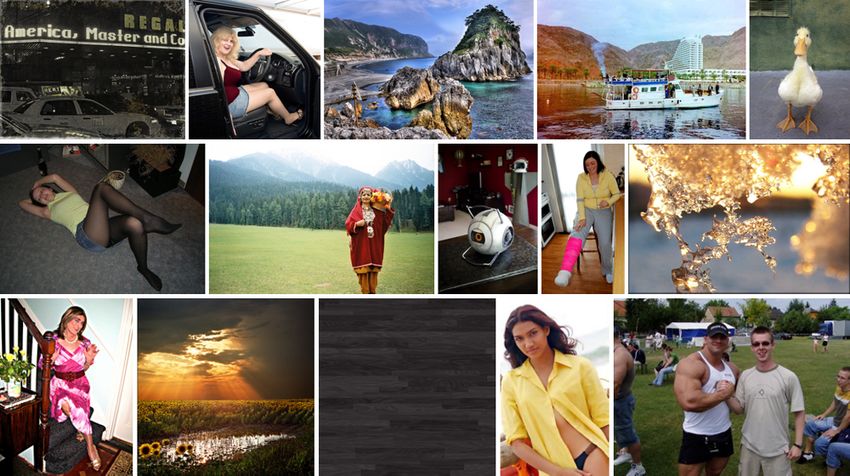
ing both image content and social cues. We consider tens of      2.   RELATED WORK
thousands of users and perform extensive evaluation based           Popularity prediction in social media has recently received
on prediction algorithms applied to three different settings:    a lot of attention from the research community. While most
one-per-user, user-mix, user-specific. In each of these cases,   of the work has focused on predicting popularity of text
we vary the number of users, and the number of images per        content, such as messages or tweets on Twitter [42, 20], and
user. In each of these cases, the relative importance of dif-    some recent works on video popularity [43, 49, 38], signifi-
ferent attributes are presented and compared against several     cantly less effort has been expended in prediction of image
baselines. We identify insights from our method that open-       popularity. The challenge and opportunity for images comes
up several directions for further exploration.                   from the fact that one may leverage both social cues (such
   We briefly summarize the main contributions of our            as the user’s context, influence etc. in the social media plat-
work in the following:                                           form), as well as image-specific cues (such as the color spec-
                                                                 trum, the aesthetics of the image, the quality of the contrast
   • We initiate a study of popularity prediction for images     etc.). Text based popularity prediction has of course lever-
     uploaded on social networks on a massive dataset from       aged the social context, as well as the content of the text
     Flickr. Our work is one of the first to investigate high-   itself. However, image content can be significantly harder
     level and low-level image features and combine them         to extract, and correlate with popularity.
     with the social context towards predicting popularity          Recently, there has been an increasing interest in ana-
     of photographs.                                             lyzing various semantic attributes of images. One such at-
                                                                 tribute is image memorability which has been shown to be
   • Combing various features, we present an approach that       an intrinsic image property [21] with different image regions
     obtains more than 0.8 rank correlation on predicting        contributing differently to an image’s memorability [29, 28].
     normalized popularity. We contrast our prediction tech-     Similarly, image quality and aesthetics are other attributes
     nique that leverages social cues and image content fea-     that have been recently explored in substantial detail [6, 8,
     tures with simpler methods that leverage color spaces,      3]. Recent work has also analyzed the more general attribute
     intensity, and simple contextual metrics. Our tech-         of image intrestingness [53], particularly focusing on its cor-
     niques highlight the importance of low-level computer       relation with image memorability [19]. There have also been
     vision features and demonstrate the power of certain        a variety of other works dealing with facial [33], scene [41]
     semantic features extracted using deep learning.            and object [14] attributes.
   • We investigate the relative importance of individual           In social context, there has been significant interest in un-
     features, and specifically contrast the power of social     derstanding behavioral aspects of users online and in social
     context with image content across three different dataset   networks. There is a large body of work studying the corre-
     types - one where each user has only one image, an-         lation of activity among friends in online communities; see
     other where each user has several thousand images,          examples in [18, 47, 48]. Most are forms of diffusion research,
     and a third where we attempt to get specific predic-        built on the premise that user engagement is contagious. As
     tors for users separately. This segmentation highlights     such, a user is more likely to adopt new products or be-
     benefits derived from the different signals and draws       haviors if their friends do so [1, 36]; and large cascades of
     insights into the contributions of popularity prediction    behavior can be triggered by the actions of a few individuals
     in comparison to simpler baseline techniques.               [18, 47]. A number of theoretical models have been devel-
                                                                 oped to model influence cascades [37, 9]. The seminal work
   • As an important contribution, this work opens the           of Kempe et al. [24] also consider two models of influence;
     doors for several interesting directions to pursue image    there has also been a long line of work on viral marketing
     popularity prediction in general, and pose broad so-        starting from [10, 46]. All these works focus on influence but
     cial questions around online behavior, popularity, and      do not necessarily predict popularity beforehand - they are
     causality. For example, while our work attempts to dis-     generic techniques that do not focus on a specific domain
     entangle social and content based features, and derives     such as images in our context.
     new insights into their predictive power, it also begs         It would be interesting to explore emotions elicited from
     the question on their impacts influencing each other        images, and their causal influence on image popularity on
     through self-selection. Our work sheds some light on        social networks - some interesting studies in other domains
     such interesting relations between features and popu-       include [23, 30].
     larity, but also poses several questions.                      In the context of social networks, there has been a great
                                                                 deal of focus on understanding the effects of friends on be-
   Paper Overview. The rest of the paper is organized as         havior. In a very interesting piece of work, Crandall et al. [4]
follows. We begin by mentioning related work in Section 2.       consider the two documented phenomenon, social influence
Section 3 describes our problem formulation by providing in-     and selection, in conjunction. They [4] suggest that users
tuition for what image popularity means, and also described      have an increased tendency to conform to their friends’ in-
the details of the dataset used throughout this paper. and       terests. Another related work [31] considers homophily in so-
methodologies. We then delve into the details of the predic-     cial networks: they conclude that users’ preference to similar
tion techniques using image content based cues and social        people is amplified over time, due to biased selection. An
cues independently in Sections 4 and 5 respectively. Our         interesting open question in our context is whether users,
main combined technique, analysis and detailed experimen-        over time, have an increasing tendency to share images that
tal evaluation are presented in Section 6. Finally, Section 7    cater to their friends’ preferences - and if yes, how this af-
concludes with a summary of our findings and a discussion        fects overall popularity. As such, our work does not delve
of several possible directions for future work.                  into these social aspects. We focus primarily on the task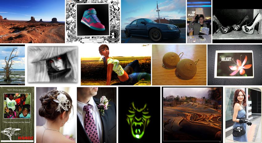
Figure 1: Sample images from our image popularity dataset. The popularity of the images is sorted from
more popular (left) to less popular (right).
0.08
0.5 0.08
of popularity prediction. It would be interesting to further
proportion of images
proportion of images
proportion of images
0.45 0.07
0.07
0.4
explore the contributions of homophily to virality of images. 0.35
0.06
0.05
0.06
0.05
0.3
0.04 0.04
0.25
0.2 0.03 0.03
0.15
3. WHAT IS IMAGE POPULARITY? 0.1
0.05
0.02
0.01
0.02
0.01
0 0
There are various ways to define the popularity of an im- 0
0 2 4 6
number of views
8 10
4
x 10
0 2 4 6 8 10
log2(number of views)
12 14 16 0 2 4 6 8 10 12
log2(normalized no. of views)
14 16
age such as the number of ‘likes’ on Facebook, the number
of ‘pins’ on Pinterest or the number of ‘diggs’ on Digg. It is Figure 2: Histogram of view counts of images. The
difficult to precisely pick any single one as the true notion different graphs show different transformations of
of popularity - different factors are likely to impact these the data: (left) absolute view counts1 , (middle) log2
different measures of popularity in different contexts. In of view counts +1 and (right) log2 view counts +1
this work, we focus on the number of views on Flickr as our normalized by upload date.
medium for exploring image popularity. Given the avail-
ability of a comprehensive API that provides a host of in-
formation about each image and user, together with a well
our algorithms in 3 different settings namely one-per-user,
established social network with significant public content,
user-mix, and user-specific. The main components that we
we are able to conduct a relatively large-scale study with
vary across these settings is the number of images per user
millions of images and hundreds of thousands of users.
in the dataset, and whether we perform user-specific pre-
Figure 2(a) shows the histogram of the number of views
dictions. These settings are described below. In the later
received by the 2.3 million(M) images used in our study. Our
sections, we will show the importance of splitting image pop-
dataset not only contains images that have received millions
ularity into these different settings by illustrating how the
of views but also plenty of images that receive zero views.
relative contribution of both content-based and social fea-
To deal with the large variation in the number of views of
tures changes across these tasks.
different images, we apply the log function as shown in Fig-
One-per-user: For this setting, we use the Visual Senti-
ure 2(b). Furthermore, as shown in [51], we know that unlike
ment Ontology dataset [3] consisting of approximately 930k
Digg, visual media tends to receive views over some period
images from about 400k users, resulting in a little over two
of time. To normalize for this effect, we divide the number
images from each user on average. This dataset was col-
of views by the duration since the upload date of the given
lected by searching Flickr for 3244 adjective-noun-pairs such
image (obtained using Flickr API). The results are shown in
as ‘happy guy’, ‘broken fence’, ‘scary cat’, etc corresponding
Figure 2(c). We find that this resembles a Gaussian distri-
to various image emotions. This dataset represents the set-
bution of the view counts as one would expect. Throughout
ting where different images belong to different users. This
the rest of this paper, image popularity refers to this log-
is often the case in search results.
normalized view count of images.
User-mix: For this setting, we randomly selected about
In the following, we provide details regarding the datasets
100 users from the one-per-user dataset that had between
used (Section 3.1), and the evaluation metric (Section 3.2)
10k and 20k public photos shared on Flickr, resulting in a
for predicting image popularity.
dataset of approximately 1.4M images. In this setting, we
put all these images from various users together and perform
3.1 Datasets popularity prediction on the full set. This setting often oc-
Figure 1 shows a sample of the images in our dataset. In curs on newsfeeds where people see multiple images from
order to explore different data distributions that occur natu- their own contacts or friends.
rally in various applications and social networks, we evaluate User-specific: For this setting, we split the dataset from
1 the user-mix setting into 100 different users and perform
Note that the maximum view count of a single image in training and evaluation independently for each user and av-
our dataset is 2.5M, but we truncate the graph on the left
to amplify the remaining signal. Despite this, it is difficult erage the results. Thus, we build user-specific models to
to see any clear signal as most images have very few views. predict the popularity of different images in their own col-
This graph is best seen on the screen with zoom. lections. This setting occurs when users are taking pictures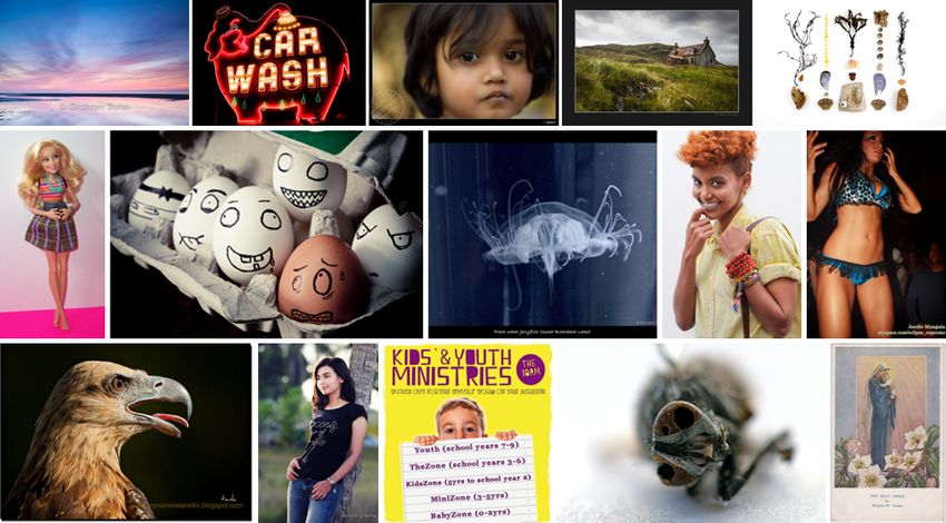
or selecting pictures to highlight - they want to pick the im-                                 rank corr = -0.05                                    rank corr = 0.02                                     rank corr = 0.01
                                                                                     20                                                    20                                                   20

                                                                  normalized views

                                                                                                                                                                             normalized views
                                                                                                                        normalized views
ages that are most likely to receive a high number of views.

3.2    Evaluation                                                                    10                                                    10                                                   10
   For each of the settings described above, we split the data
randomly into two halves, one for training and the other
testing. We average the performance over 10 random splits                              0
                                                                                           0            0.5         1
                                                                                                                                            0
                                                                                                                                                0         0.5            1
                                                                                                                                                                                                 0
                                                                                                                                                                                                     0           0.5         1
to ensure the consistency of our results; overall, we find that                                   mean hue                                          mean saturation                                         mean value
our results are highly consistent with low standard devia-                       18            rank corr = -0.00                        18          rank corr = 0.01                            20       rank corr = -0.02

                                                                                                                         normalized views

                                                                                                                                                                              normalized views
                                                                  normalized views
tions across splits. We report performance in terms of Spear-
man’s rank correlation (ρ) between the predicted popularity
and the actual popularity. Note that we use log-normalized                             9                                                    9                                                    8

view count of images as described in the beginning of this
section for both training and testing. Additionally, we found
                                                                                       0                                                    0                                                    -5
that rank correlation and standard correlation give very sim-                              0             0.5        1                        0            0.125        0.25                       -50             50        150
ilar results.                                                                                   intensity mean                                      intensity variance                               intensity skewness

4.    PREDICTING POPULARITY USING
                                                                  Figure 3: Correlation of popularity with different
      IMAGE CONTENT                                               components of the HSV color space (top), and in-
  In this section, we investigate the use of various features     tensity statistics (bottom).
based on image content that could be used to explain the
popularity of images. First, in Section 4.1 we investigate
                                                                                       6
some simple human-interpretable features such as color and
intensity variance. Then, in Section 4.2, we explore some                              5
low-level computer vision features inspired by how humans           color importance
perceive images such as gradient, texture or color patches.                            4

Last, in Section 4.3, we explore some high-level image fea-                            3
tures such as the presence of various objects. Experimen-
tal results show that low-level computer vision features and                           2

high-level semantic features tend to be significantly more
                                                                                       1
predictive of image popularity than simple image features.
                                                                                       0
4.1    Color and simple image features
   Are simple image features enough to determine whether                                            5          10       15                          20     25     30                      35                40         45    50

or not an image will be popular? To address this, we evalu-                                                                                              colors
ate the rank correlation between popularity and basic pixel
statistics such as the mean value of different color channels     Figure 4: Importance of different colors to predict
in HSV space, and intensity mean, variance, and skewness.         image popularity. The length of each bar shows im-
The results are shown in Figure 3. We find that most sim-         portance of the color shown on the bar.
ple features have very little correlation with popularity, with
mean saturation having the largest absolute value of 0.05.
Here, we use all 2.3M images independent of the settings          bluish colors tend to have lower importance as compared
described in Section 3.1. Since significant correlation does      to more reddish colors. This might occur because images
not exist between simple image features and popularity, we        containing more striking colors tend to catch the eye of the
omit results from the individual settings for brevity.            observer leading to a higher number of views.
   Additionally, we look at another simple feature: the color        While the simple features presented above are informa-
histogram of images. As the space of all colors is very large     tive, more descriptive features are likely necessary to better
(256 ∗ 256 ∗ 256 ≈ 16.8m), and since small variations in          represent the image in order to make better predictions. We
lighting and shadows can drastically change pixel values,         explore these in the remaining part of this section.
we group the color space into 50 distinct colors as described
in [26] to be more robust to these variations. Then, we assign    4.2                             Low-level computer vision features
each pixel of the image to one of these 50 colors and form a
                                                                     Motivated by Khosla et al. [29, 27], we use various low-
`1 -normalized histogram of colors. Using support vector re-
                                                                  level computer vision features that are likely used by hu-
gression (SVR) [12] with a linear kernel (implemented using
                                                                  mans for visual processing. In this work, we consider five
LIBLINEAR [13]), we learn the importance of these colors
                                                                  such features namely gist, texture, color, gradient and deep
in predicting image popularity2 . The results are shown in
                                                                  learning features. For each of the features, we describe our
Table 1 (column: color histogram), and visualized in Fig-
                                                                  motivation and the method used for extraction below.
ure 4. Despite its simplicity, we obtain a rank correlation of
                                                                     Gist: Various experimental studies [44, 2] have suggested
0.12 to 0.23 when using this feature on the three different
                                                                  that the recognition of scenes is initiated from the encoding
data settings. We observe that on average, the greenish and
                                                                  of the global configuration, or spatial envelope of the scene,
2                                                                 overlooking all of the objects and details in the process. Es-
  We find the hyperparameter C ∈ {0.01, 0.1, 1, 10, 100} us-
ing five-fold cross-validation on the training set.               sentially, humans can recognize scenes just by looking at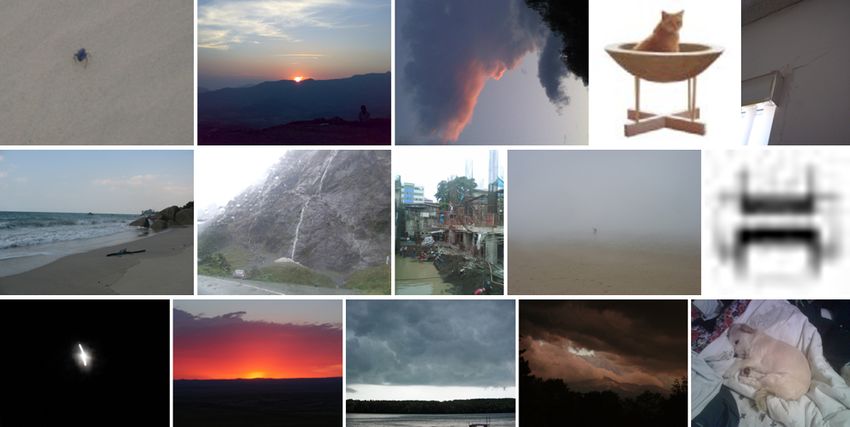
Dataset           Gist   Color histogram    Texture     Color patches               Gradient     Deep learning   Objects   Combined
    One-per-user      0.07         0.12          0.20           0.23                      0.26           0.28         0.23       0.31
    User-mix          0.13         0.15          0.22           0.29                      0.32           0.33         0.30       0.36
    User-specific     0.16         0.23          0.32           0.36                      0.34           0.26         0.33       0.40

                    Table 1: Prediction results using image content only as described in Section 4.

their ‘gist’. To encode this, we use the popular GIST [40]                                color patches
descriptor with a feature dimension of 512.
                                                                                          color histograms
   Texture: We routinely interact with various textures and
                                                                                          gist
materials in our surroundings both visually, and through

                                                                     rank correlation
touch. To test the importance of this type of feature in                                  gradient
predicting image popularity, we use the popular Local Bi-                                 texture
nary Pattern (LBP) [39] feature. We use non-uniform LBP
pooled in a 2-level spatial pyramid [34] resulting in a feature
of 1239 dimensions.
   Color patches: Colors are a very important component
of human visual system for determining properties of ob-
jects, understanding scenes, etc. The space of colors tends
to have large variations by changes in illumination, shad-
ows, etc, and these variations make the task of robust color
                                                                                                             user index
identification difficult. While difficult to work with, var-
ious works have been devoted to developing robust color
descriptors [54, 26], which have been proven to be valuable          Figure 5: Prediction performance of different fea-
in computer vision for various tasks including image classi-         tures for 20 random users from the user-specific set-
fication [25]. In this paper, we use the 50 colors proposed          ting. This figure is best viewed in color.
by [26] in a bag-of-words representation. We densely sample
them in a grid with a spacing of 6 pixels, at multiple patch
sizes (6, 10 and 16). Then we learn a dictionary of size 200         columns, the rank correlation performance is best for the
and apply LLC [55] together with max-pooling in a 2-level            user-specific dataset, and next for user-mix, followed by one-
spatial pyramid [34] to obtain a final feature vector of 4200        per-user. However, it is important to note that the predic-
dimensions.                                                          tion accuracy when all the features are combined (as seen
   Gradient: In the human visual system, much evidence               in the last column in Table 1) is at least 0.30 in all three
suggests that retinal ganglion cells and cells in the visual         cases. Given that these results only leverage image-content
cortex V1 are essentially gradient-based features. Further-          features (therefore ignore any aspects of the social platform
more, gradient based features have been successfully applied         or user-specific attributes), the correlation is very signifi-
to various applications in computer vision [5, 15]. In this          cant. While most of the current research focuses solely on
work, we use the powerful Histogram of Oriented Gradi-               the social network aspect when predicting popularity, this
ent (HOG) [5] features combined with a bag-of-words rep-             result suggests that the content also plays a crucial role, and
resentation for popularity prediction. We sample them in a           may provide complementary information to the social cues.
dense grid with a spacing of 4 pixels for adjacent descriptors.         On exploring the columns individually in Table 1, we no-
Then we learn a dictionary of size 256, and apply Locality-          tice that the color histogram alone gives a fairly low rank
Constrained Linear Coding (LLC) [55] to assign the descrip-          correlation (ranging between 0.12 and 0.23 across the three
tors to the dictionary. We finally concatenate descriptors           datasets), but texture, and gradient features perform sig-
from multiple image regions (max-pooling + 2-level spatial           nificantly better (improving the performance ranges to 0.20
pyramid) as described in [34] to obtain a final feature of           to 0.32 and 0.26 to 0.34 respectively). The deep learning
10, 752 dimensions.                                                  features outperform other features for the one-per-user and
   Deep learning: Deep learning algorithms such as convo-            user-mix settings but not the user-specific setting. We then
lutional neural networks (CNNs) [35] have recently become            combine features by training a SVR on the output of the
popular as methods for learning image representations [32].          SVR trained on the individual features. This finally pushes
CNNs are inspired by biological processes as a method to             the range of the rank correlations to 0.31 to 0.40.
model the neurons in the brain, and have proven to gener-               In conjunction with the aggregate evaluation metrics de-
ate effective representation of images. In this paper, we use        scribed above and presented in Table 1, it is informative
the recently popular ‘ImageNet network’ [32] trained on 1.3          to look at the specific performance across 20 randomly se-
million images from the ImageNet [7] challenge 2012. Specif-         lected users from the user-specific setting for each of these
ically, we use Decaf [11] to extract features from the layer         features - this is presented in a rank correlation vs. user in-
just before the final 1000 class classification layer, resulting     dex scatter plot in Figure 5. The performance for all features
in a feature of 4096 dimensions.                                     combined is not displayed here to demonstrate the specific
   Results: As described in Section 4.1, we train a lin-             variance across the image cues. As can be seen here, the
ear SVR to perform popularity prediction on the different            color patches (red dots) performs best nearly consistently
datasets. The results averaged over 10 random splits are             across all the users. For a couple of users, the gradient (black
summarized in Table 1. As can be seen from any of the                dots) performs better, and for others performs nearly as well
                                                                     as the color patches. In both these features, the prediction
Mean    Photo                            Group     Member                       Title     Desc.
      Dataset                           Contacts     Groups                           Is pro?   Tags                       All
                        Views   Count                           members    duration                    length    length
      One-per-user       0.75    0.07      0.46       0.27        0.27      -0.08      0.22     0.52    0.21      0.45    0.77
      User-mix           0.62   -0.05      0.26       0.24        0.06      -0.01      0.07     0.40    0.29      0.35    0.66
      User-specific      n/a     n/a       n/a        n/a         n/a        n/a       n/a      0.19    0.16      0.19    0.21

                      Table 2: Prediction results using social content only as described in Section 5.

accuracy is fairly consistent. On the other hand, gist has           It is interesting to observe that this is similar to what we
a larger variance and the lowest average rank correlation.           might expect. It is important to note that this object clas-
From the figure, it can be seen that texture (pink dots) also        sifier is not perfect, and may often wrongly classify images
plays a vital role in predicting rank correlation accuracy, as       to contain certain objects that they do not. Furthermore,
it spans the performance range of roughly 0.22 to 0.58 across        there may be certain object categories that are present in
the randomly sampled users.                                          images but not in the 1000 objects the classifier recognizes.
   Another point of Figure 5 is to show that for personaliza-        This object-popularity correlation might therefore not pick
tion (i.e. user specific experiments), different features may        up on some important object factors. However in general,
be indicative of what a user’s social network likes (because         our analysis is still informative and intuitive about what
that is essentially what the model will capture by learning          type of objects might play a role in a picture’s popularity
a user-specific model based on the current set of images). It
is therefore interesting to note some variation in importance        5.    PREDICTING POPULARITY USING
or relative ranking of features across the sampled users.
                                                                           SOCIAL CUES
4.3     High-level features: objects in images                          While image content is useful to predict image popularity
   In this section, we explore some high-level or semantically       to some extent, social cues play a significant role in the num-
meaningful features of images, namely the objects in an im-          ber of views an image will receive. A person with a larger
age. We want to evaluate whether the presence or absence             number of contacts would naturally be expected to receive a
of certain objects affects popularity e.g. having people in an       higher number of average views. Similarly, we would expect
image might make it more popular as compared to having               that an image with more tags shows up in search results
a bottle. Given the scale of the problem, it is difficult and        more often (assuming each tag is equally likely). Here, we
costly to annotate the dataset manually. Instead, we can use         attempt to quantify the extent to which the different social
a computer vision system to roughly estimate the set of ob-          cues impact the popularity of an image.
jects present in an image. Specifically, we use the deep learn-         For this purpose, we consider several user-specific or so-
ing classifier [32] described in the previous subsection that        cial context specific features. We refer to user features as
distinguishes between 1000 object categories ranging from            ones that are shared by all images of a single user. The
lipstick to dogs to castle. In addition, this method achieved        user features that we use in our analysis are listed and de-
state-of-the-art classification results in the ImageNet classifi-    scribed below. Note that this work investigates the relative
cation challenge demonstrating its effectiveness in this task.       merits of social and image features, and the goal isn’t to
We treat the output of this 1000 object classifier as features,      heavily exploit one. Thus, we use relatively simple features
and train a SVR to predict log-normalized image popularity           for social cues that could likely be improved by using more
as done in the previous sections. The results are summarized         sophisticated approaches.
in Table 1.                                                               • Mean Views: mean of number of normalized views
   We observe that the presence or absence of objects is a                  of all public images of the given user
fairly effective feature for predicting popularity for all three
settings with the best performance achieved in user-specific              • Photo count: number of public images uploaded by
case. Further, we investigate the type of objects leading                   the given user
to image popularity. On the one-per-user dataset, we find                 • Contacts: number of contacts of the given user
that some of the most common objects present in images
are: seashore, lakeside, sandbar, valley, volcano. In order to            • Groups: number of groups the given user belongs to
evaluate the correlation of objects with popularity, we com-              • Group members: average number of members in the
pute the mean of the SVR weights across the 10 train/test                   groups a given user belongs to
splits of the data, and sort them. The resulting set of objects
with different impact on popularity is as follows:                        • Member duration: the amount of time since the
                                                                            given user joined Flickr
   • Strong positive impact: miniskirt, maillot, bikini,
     cup, brassiere, perfume, revolver                                    • Is pro: whether the given user has a Pro Flickr ac-
                                                                            count or not
   • Medium positive impact: cheetah, giant panda,                      We further subdivide some of the above features such as
     basketball, llama, plow, ladybug                                ‘groups’ into number of groups a given user is an adminis-
   • Low positive impact: wild boar, solar dish, horse               trator of, and the number of groups that are ‘invite only’.
     cart, guacamole, catamaran                                      We also include some image specific features that refer to
                                                                     the context (i.e. supporting information associated with the
   • Negative impact: spatula, plunger, laptop, golfcart,            image as entered by the user but not its pixel content, as
     space heater                                                    explored in Section 4). These are listed below.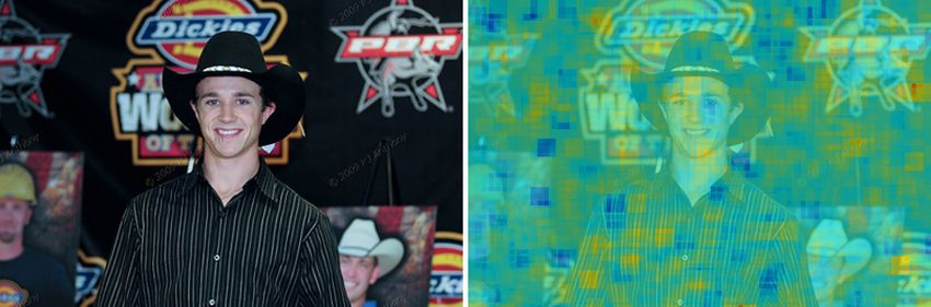
• Tags: number of tags of the image Dataset Content Social Content +
only only Social
• Title length: length of the image title One-per-user 0.31 0.77 0.81
• Desc. length: length of the image description User-mix 0.36 0.66 0.72
User-specific 0.40 0.21 0.48
For each of the above features, we find its rank correla-
tion with log-normalized image popularity. The results are
Table 3: Prediction results using image content and
shown in Table 2. Note that the user features such as Mean
social cues as described in Section 6.1.
Views and Contacts would have the same value for all im-
ages by the particular user in the dataset. Not surprisingly,
in the one-per-user dataset, the Mean Views feature per- 6. ANALYSIS
forms extremely well in predicting the popularity of a new
In this section, we further analyze some of our results from
image with a rank correlation of 0.75. However, the rank
the previous sections. First, we combine the signal provided
correlation drops to 0.62 on the user-mix setting because
by image content and social cues in Section 6.1. We observe
there is no differentiation between a user’s photos.
that both of these modalities provide some complementary
That said, 0.75 rank correlation is still a significantly bet-
signal and can be used together to improve popularity pre-
ter performance than we had expected since we note that the
diction further. In Section 6.2 we visualize the good and bad
mean of views was taken over all public photos of the given
predictions made by our regressors in an attempt to better
user, not just the ones in our dataset. The mean number
understand the underlying model. Last, in Section 6.3 we
of public photos per user is over 1000, and of these, typ-
show some preliminary visualizations of the image regions
ically 1-2 are in our dataset, so this is a fairly interesting
that make images popular by reversing the learned weights
observation.
and applying them to image regions.
Another noteworthy feature is contacts - we see a rank
correlation for these two datasets to be 0.46 and 0.26 re-
spectively i.e. the more contacts a user has, the higher the
6.1 Combining image content and social cues
popularity of their images. This is to be expected as their We combine the output of the image content and social
photos would tend to be highlighted for a larger number of cues using a SVR trained on the outputs of the most ba-
people (i.e. their social network). Further, we observe that sic features, commonly referred to as late fusion. Table 3
the image-specific social features such as tags, title length, shows the resulting performance. We observe that the per-
and description length are also good predictors for popular- formance improves significantly for all 3 datasets as com-
ity. As we can see in Table 2, their performance across the pared to using either sets of features independently. The
three dataset types range from 0.19 to 0.52 for tags, and 0.19 smallest increase of 0.04 rank correlation is observed for the
to 0.45 for description length. This is again to be expected as one-per-user dataset as it already has a fairly high rank
having more tags or a longer description/title increases the correlation largely contributed by the social features. This
likelihood of these images appearing in the search results. makes it difficult to improve performance further by using
Further, we combine all the social features by training a content features, but it is interesting to observe that we can
SVR with all the social features as input. The results are predict the number of views in this setting with a fairly high
shown in the rightmost column of Table 2. In this case, we rank correlation of 0.81. We observe the largest gains in the
see a rank correlation of 0.21, 0.66, and 0.77 for the user- user-specific dataset, of 0.08 rank correlation, where image
specific, user-mix, and one-per-user datasets respectively. content features play a much bigger role as compared to
Thus, it is helpful to combine the social features, but we social features.
observe that the performance does not increase very signif-
icantly as compared to the most dominant feature. This 6.2 Visualizing results
suggests that many of these features are highly correlated In Figure 6, we visualize some of the good and bad pre-
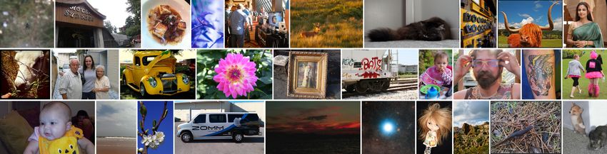
and do not provide complementary information. dictions made using our regressors. We show the four main
To contrast the results of social features from Table 2 with quadrants: two with green background where the high or
the image content features presented in the previous section low popularity prediction matches the ground truth, and
in Table 1, we observe that the social features tend to per- two with green background where the prediction is either
form better in the one-per-user and user-mix dataset types, too high or too low. We observe that images with low pre-
while the image content features perform better in the user- dicted scores (bottom half) tend to be less ‘busy’ and pos-
specific dataset type. We suspect that in the user-specific sibly lack interesting features. They tend to contain clean
dataset, where each user has thousands of images, the im- backgrounds with little to no salient foreground objects, as
portance of personalized social cues becomes less relevant compared to the high popularity images. Further, we ob-
(perhaps due to the widespread range of images uploaded serve that the images with low popularity but predicted to
by them) and so the image content features become partic- have high popularity (top-left quadrant) tend to resemble
ularly relevant. the highly popular images (top-right quadrant) but may not
One thing that is evident from these results is that the so- be popular due to the social network effects of the user. In
cial features and image content features are both necessary, general, our method tends to do relatively well in picking
and offer individual insights that are not subsumed by each images that could potentially have a high number of views
other i.e. the choice of features for different applications regardless of social context.
largely depends on the data distribution. In the following
section, we investigate techniques combining both of these 6.3 Visualizing what makes an image popular
features that turn out to be more powerful and perform well To better understand what makes an image popular, we
across the spectrum of datasets. attempt to attribute the popularity of an image to its re-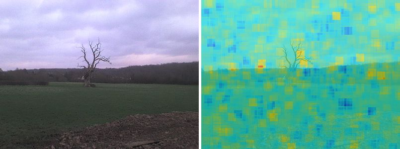
gions (similar to [29]). Being able to visualize the regions
that make an image popular can be extremely useful in a
variety of applications e.g. we could teach users to take bet-
ter photographs by highlighting the important regions, or
modify images automatically to make them more popular
by replacing the regions with low impact on popularity.
   In Figure 7, we visualize the contribution of different im-
age regions to the popularity of an image by reversing the
contribution of the learned weights to image descriptors.
Since we use a bag-of-words descriptor, it can be difficult
to identify exactly which descriptors in the image are con-
tributing positively or negatively to the popularity score.
Since max-pooling is used over spatial regions, we can care-
fully record the descriptors and their locations that led to
the maximum value for each bag-of-words dictionary ele-
ment. Then, we can combine this with the weights learned
by SVR to generate a ‘heatmap’ of the regions that make an       Figure 7: Popularity score of different image regions
image popular. Note that this is a rather coarse heatmap         for images at different levels of popularity: high (top
because there can be image descriptors that have high val-       row), medium (middle row) and low (bottom row).
ues for certain dictionary elements, but not the highest, and    The importance of the regions decreases in the order
their contribution is not considered in this max-pooling sce-    red > green > blue.
nario. Thus, we end up with heatmaps that do not look
semantically pleasing but indicate regions of high or low
interest rather coarsely. This representation could be im-
                                                                    Several directions remain for future exploration. An inter-
proved by using the recently popular mid-level features [50,
                                                                 esting question is predicting shareability as opposed to pop-
22] which encode more semantically meaningful structure.
                                                                 ularity. Are these different traits? There might be some im-
   From Figure 7, we can see that semantically meaningful
                                                                 ages that are viewed/consumed, but not necessarily shared
objects such as people tend to contribute positively to the
                                                                 with friends. Does this perhaps have a connection with the
popularity of an image (first row right, and second row).
                                                                 emotion that is elicited? For example, peaceful images may
Further we note that open scenes with little activity tend
                                                                 get liked, funny images may get shared, and scary/disturbing
to be unpopular (with many exceptions of course). We ob-
                                                                 images may get viewed but not publicly broadcasted. It
serve that the number of high-scoring red/yellow regions de-
                                                                 would be interesting to understand the features/traits that
crease as the popularity of an image decreases (bottom row).
                                                                 distinguish the kinds of interaction they elicit from users.
Further, we observe that several semantically meaningful
                                                                 vs. those that elicit more uniform responses.
objects in the images are highlighted such as the train or
                                                                    On a more open-ended note, do the influence of social
different body parts, but due to the shortcoming described
                                                                 context and image content spill across their boundaries? It
earlier, the regions are incoherent and broken up into several
                                                                 is conceivable that a user who uploads refined photographs,
parts. Overall, popularity is a difficult metric to understand
                                                                 over time, accumulates a larger number of followers. This
precisely based on image content alone because social cues
                                                                 could garner a stronger influence through the network and
have a large influence on the popularity of images.
                                                                 thereby result in increased popularity of photos uploaded by
                                                                 this user. Attribution might be inaccurate as a consequence
                                                                 - the resulting popularity may be ascribed to the user’s social
7.   CONCLUSIONS AND FUTURE WORK                                 context and miss the image content. Popularity prediction
   In this paper, we explored what makes images uploaded         as such may not be adversely affected, but what is the right
by users popular among online social media. Specifically,        causality here? Disentangling these features promises for an
we explored millions of images on Flickr uploaded by tens        exciting direction to take this research forward. Being able
of thousands of users and studied the problem of predicting      to disentangle these factors may also result in improved con-
the popularity of of the uploaded images. While some im-         tent based popularity prediction by removing noise from the
ages get millions of views, others go completely unnoticed.      labels caused by social factors. Another specific question,
This variation is noticed even among images uploaded by the      for which data is unfortunately unavailable, is understand-
same user, or images from the same genre. We designed an         ing time series of popularity for images: rather than simply
approach that leverages social cues as well as image content     looking at total popularity (normalized or unnormalized),
features to come up with a prediction technique for over-        can one investigate temporal gradients as well? For exam-
all popularity. We also show key insights from our method        ple, the total popularity of two images (or classes of images)
that suggest crucial aspects of the image that determine or      may be the same, yet, one may have rapidly gained popular-
influence popularity. We extensively test our methodology        ity and then sharply fallen, while another might have slowly
across different dataset types that have a variable distribu-    and constantly retained popularity. These could perhaps
tion of images per user, as well as explore prediction models    exhibit fundamentally different photograph-types, perhaps
that are focused on certain user groups or independent users.    the former being due to a sudden news or attention on an
The results show interesting variation in importance of so-      event, figure, or location, while the latter due to some intrin-
cial cues such as number of photos uploaded or number of         sic lasting value. Such exploration would be really valuable
contacts, and contrast it with image cues such as color or       and exciting if the time series data were available for up-
gradients, depending on the dataset types.                       loaded images.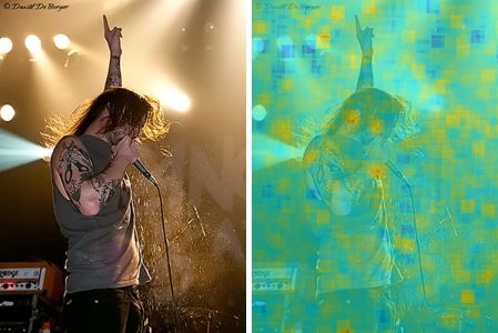
predicted popularity

                                                                                             ground truth popularity

Figure 6: Predictions on some images from our dataset using Gradient based image predictor. We show
four quadrants of ground truth popularity and predicted popularity. The green and red background colors
represent correct and false predictions respectively.

  Finally, from an application standpoint, is there a photog-       [5] N. Dalal and B. Triggs. Histograms of oriented gradients
raphy popularity tool that could be built here? Can pho-                for human detection. In Computer Vision and Pattern
tographers be aided with suggestions on how to modify their             Recognition, 2005. CVPR 2005. IEEE Computer Society
                                                                        Conference on, volume 1, pages 886–893. IEEE, 2005.
pictures for broad appeal vs artistic appeal? This could be
                                                                    [6] R. Datta, J. Li, and J. Z. Wang. Algorithmic inferencing of
an interesting research direction as well as a promising prod-          aesthetics and emotion in natural images: An exposition. In
uct. This is to be contrasted with some recent work3 on                 Image Processing, 2008. ICIP 2008. 15th IEEE
aided movie script writing tools, where machine learning is             International Conference on, pages 105–108. IEEE, 2008.
potentially used to predict the likelihood of viewers enjoying      [7] J. Deng, W. Dong, R. Socher, L.-J. Li, K. Li, and
the movie plot.                                                         L. Fei-Fei. ImageNet: A Large-Scale Hierarchical Image
                                                                        Database. In CVPR09, 2009.
                                                                    [8] S. Dhar, V. Ordonez, and T. L. Berg. High level describable
Acknowledgments                                                         attributes for predicting aesthetics and interestingness. In
Aditya Khosla is supported by a Facebook Fellowship.                    Computer Vision and Pattern Recognition (CVPR), 2011
                                                                        IEEE Conference on, pages 1657–1664. IEEE, 2011.
                                                                    [9] P. S. Dodds and D. J. Watts. A generalized model of social
8.   REFERENCES                                                         and biological contagion. Journal of Theoretical Biology,
 [1] L. Backstrom, D. Huttenlocher, J. Kleinberg, and X. Lan.           2005.
     Group formation in large social networks: membership,         [10] P. Domingos and M. Richardson. Mining the network value
     growth, and evolution. In KDD ’06, pages 44–54, 2006.              of customers. In KDD, pages 57–66, 2001.
 [2] I. Biederman. Aspects and extensions of a theory of human     [11] J. Donahue, Y. Jia, O. Vinyals, J. Hoffman, N. Zhang,
     image understanding. Computational processes in human              E. Tzeng, and T. Darrell. Decaf: A deep convolutional
     vision: An interdisciplinary perspective, pages 370–428,           activation feature for generic visual recognition. arXiv
     1988.                                                              preprint arXiv:1310.1531, 2013.
 [3] D. Borth, R. Ji, T. Chen, T. Breuel, and S.-F. Chang.         [12] H. Drucker, C. J. Burges, L. Kaufman, A. Smola, and
     Large-scale visual sentiment ontology and detectors using          V. Vapnik. Support vector regression machines. Advances
     adjective noun pairs. In ACM MM, 2013.                             in neural information processing systems, pages 155–161,
 [4] D. J. Crandall, D. Cosley, D. P. Huttenlocher, J. M.               1997.
     Kleinberg, and S. Suri. Feedback effects between similarity   [13] R.-E. Fan, K.-W. Chang, C.-J. Hsieh, X.-R. Wang, and
     and social influence in online communities. In KDD, pages          C.-J. Lin. Liblinear: A library for large linear classification.
     160–168, 2008.                                                     The Journal of Machine Learning Research, 9:1871–1874,
3                                                                       2008.
  http://www.nytimes.com/2013/05/06/business/media/solving-
equation-of-a-hit-film-script-with-data.html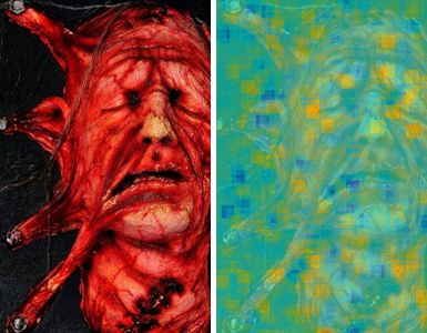
[14] A. Farhadi, I. Endres, D. Hoiem, and D. Forsyth.                        scene categories. In Computer Vision and Pattern
     Describing objects by their attributes. In Computer Vision              Recognition, 2006 IEEE Computer Society Conference on,
     and Pattern Recognition, 2009. CVPR 2009. IEEE                          volume 2, pages 2169–2178. IEEE, 2006.
     Conference on, pages 1778–1785. IEEE, 2009.                      [35]   Y. LeCun and Y. Bengio. Convolutional networks for
[15] P. F. Felzenszwalb, R. B. Girshick, D. McAllester, and                  images, speech, and time series. The handbook of brain
     D. Ramanan. Object detection with discriminatively                      theory and neural networks, 3361, 1995.
     trained part-based models. Pattern Analysis and Machine          [36]   J. Leskovec, L. A. Adamic, and B. A. Huberman. The
     Intelligence, IEEE Transactions on, 32(9):1627–1645, 2010.              dynamics of viral marketing. ACM Trans. Web, 1(1), 2007.
[16] F. Figueiredo. On the prediction of popularity of trends         [37]   M. E. J. Newman. Spread of epidemic disease on networks.
     and hits for user generated videos. In Proceedings of the               Physical Review E, 2002.
     sixth ACM international conference on Web search and             [38]   A. O. Nwana, S. Avestimehr, and T. Chen. A latent social
     data mining, pages 741–746. ACM, 2013.                                  approach to youtube popularity prediction. CoRR,
[17] F. Figueiredo, F. Benevenuto, and J. M. Almeida. The tube               abs/1308.1418, abs/1308.1418, 2013.
     over time: characterizing popularity growth of youtube           [39]   T. Ojala, M. Pietikainen, and T. Maenpaa. Multiresolution
     videos. In Proceedings of the fourth ACM international                  gray-scale and rotation invariant texture classification with
     conference on Web search and data mining, pages 745–754.                local binary patterns. Pattern Analysis and Machine
     ACM, 2011.                                                              Intelligence, IEEE Transactions on, 24(7):971–987, 2002.
[18] M. Gladwell. The Tipping Point: How Little Things Can            [40]   A. Oliva and A. Torralba. Modeling the shape of the scene:
     Make a Big Difference. Back Bay Books, 2002.                            A holistic representation of the spatial envelope.
[19] M. Gygli, H. Grabner, H. Riemenschneider, F. Nater, and                 International journal of computer vision, 42(3):145–175,
     L. Van Gool. The interestingness of images. In IEEE                     2001.
     ICCV, 2013.                                                      [41]   G. Patterson and J. Hays. Sun attribute database:
[20] L. Hong, O. Dan, and B. D. Davison. Predicting popular                  Discovering, annotating, and recognizing scene attributes.
     messages in twitter. In WWW (Companion Volume), pages                   In Computer Vision and Pattern Recognition (CVPR),
     57–58, 2011.                                                            2012 IEEE Conference on, pages 2751–2758. IEEE, 2012.
[21] P. Isola, J. Xiao, A. Torralba, and A. Oliva. What makes         [42]   S. Petrovic, M. Osborne, and V. Lavrenko. Rt to win!
     an image memorable? In Computer Vision and Pattern                      predicting message propagation in twitter. In ICWSM,
     Recognition (CVPR), 2011 IEEE Conference on, pages                      2011.
     145–152. IEEE, 2011.                                             [43]   H. Pinto, J. M. Almeida, and M. A. Gonçalves. Using early
[22] M. Juneja, A. Vedaldi, C. Jawahar, and A. Zisserman.                    view patterns to predict the popularity of youtube videos.
     Blocks that shout: Distinctive parts for scene classification.          In WSDM, pages 365–374, 2013.
     In Proceedings of the IEEE Conf. on Computer Vision and          [44]   M. Potter. Meaning in visual search. Science, 1975.
     Pattern Recognition (CVPR), volume 1, 2013.                      [45]   A. Rabinovich, A. Vedaldi, C. Galleguillos, E. Wiewiora,
[23] S. D. Kamvar and J. Harris. We feel fine and searching the              and S. Belongie. Objects in context. In Computer Vision,
     emotional web. In WSDM, pages 117–126, 2011.                            2007. ICCV 2007. IEEE 11th International Conference on,
[24] D. Kempe, J. Kleinberg, and E. Tardos. Maximizing the                   pages 1–8. IEEE, 2007.
     spread of influence through a social network. In KDD,            [46]   M. Richardson and P. Domingos. Mining knowledge-sharing
     pages 137–146, 2003.                                                    sites for viral marketing. In KDD, pages 61–70, 2002.
[25] F. S. Khan, J. Weijer, A. D. Bagdanov, and M. Vanrell.           [47]   E. M. Rogers. Diffusion of Innovations. Simon and
     Portmanteau vocabularies for multi-cue image                            Schuster, 2003.
     representation. In Advances in neural information                [48]   D. M. Romero, B. Meeder, and J. Kleinberg. Differences in
     processing systems, pages 1323–1331, 2011.                              the mechanics of information diffusion. In WWW ’11, 2011.
[26] R. Khan, J. Van de Weijer, F. S. Khan, D. Muselet,               [49]   D. A. Shamma, J. Yew, L. Kennedy, and E. F. Churchill.
     C. Ducottet, and C. Barat. Discriminative color                         Viral actions: Predicting video view counts using
     descriptors. CVPR, 2013.                                                synchronous sharing behaviors. In ICWSM, 2011.
[27] A. Khosla, W. A. Bainbridge, A. Torralba, and A. Oliva.          [50]   S. Singh, A. Gupta, and A. A. Efros. Unsupervised
     Modifying the memorability of face photographs. In                      discovery of mid-level discriminative patches. In Computer
     International Conference on Computer Vision (ICCV),                     Vision–ECCV 2012, pages 73–86. Springer, 2012.
     2013.                                                            [51]   G. Szabo and B. A. Huberman. Predicting the popularity
[28] A. Khosla, J. Xiao, P. Isola, A. Torralba, and A. Oliva.                of online content. Communications of the ACM,
     Image memorability and visual inception. In SIGGRAPH                    53(8):80–88, 2010.
     Asia 2012 Technical Briefs. ACM, 2012.                           [52]   A. Torralba, K. P. Murphy, W. T. Freeman, and M. A.
[29] A. Khosla, J. Xiao, A. Torralba, and A. Oliva.                          Rubin. Context-based vision system for place and object
     Memorability of image regions. In Advances in Neural                    recognition. In Computer Vision, 2003. Proceedings. Ninth
     Information Processing Systems, pages 305–313, 2012.                    IEEE International Conference on, pages 273–280. IEEE,
[30] S. Kim, J. Bak, and A. H. Oh. Do you feel what i feel?                  2003.
     social aspects of emotions in twitter conversations. In          [53]   N. Turakhia and D. Parikh. Attribute dominance: What
     ICWSM, 2012.                                                            pops out? In IEEE ICCV, 2013.
[31] G. Kossinets and D. J. Watts. Origins of homophily in an         [54]   J. Van De Weijer, C. Schmid, and J. Verbeek. Learning
     evolving social network1. American Journal of Sociology,                color names from real-world images. In Computer Vision
     115(2):405–450, 2009.                                                   and Pattern Recognition, 2007. CVPR’07. IEEE
[32] A. Krizhevsky, I. Sutskever, and G. Hinton. Imagenet                    Conference on, pages 1–8. IEEE, 2007.
     classification with deep convolutional neural networks. In       [55]   J. Wang, J. Yang, K. Yu, F. Lv, T. Huang, and Y. Gong.
     Advances in Neural Information Processing Systems 25,                   Locality-constrained linear coding for image classification.
     pages 1106–1114, 2012.                                                  In Computer Vision and Pattern Recognition (CVPR),
[33] N. Kumar, A. C. Berg, P. N. Belhumeur, and S. K. Nayar.                 2010 IEEE Conference on, pages 3360–3367. IEEE, 2010.
     Attribute and simile classifiers for face verification. In
     Computer Vision, 2009 IEEE 12th International
     Conference on, pages 365–372. IEEE, 2009.
[34] S. Lazebnik, C. Schmid, and J. Ponce. Beyond bags of
     features: Spatial pyramid matching for recognizing natural
You can also read