INDUCTIVE REPRESENTATION LEARNING IN TEMPO- RAL NETWORKS VIA CAUSAL ANONYMOUS WALKS

Under review as a conference paper at ICLR 2021

I NDUCTIVE R EPRESENTATION L EARNING IN T EMPO -
RAL N ETWORKS VIA C AUSAL A NONYMOUS WALKS

 Anonymous authors
 Paper under double-blind review

 A BSTRACT

 Temporal networks serve as abstractions of many real-world dynamic systems.
 These networks typically evolve according to certain laws, such as the law of triadic
 closure, which is universal in social networks. Inductive representation learning
 of temporal networks should be able to capture such laws and further be applied
 to systems that follow the same laws but have not been unseen during the training
 stage. Previous works in this area depend on either network node identities or rich
 edge attributes and typically fail to extract these laws. Here, we propose Causal
 Anonymous Walks (CAWs) to inductively represent a temporal network. CAWs are
 extracted by temporal random walks and work as automatic retrieval of temporal
 network motifs to represent network dynamics while avoiding the time-consuming
 selection and counting of those motifs. CAWs adopt a novel anonymization strategy
 that replaces node identities with the hitting counts of the nodes based on a set
 of sampled walks to keep the method inductive, and simultaneously establish the
 correlation between motifs. We further propose a neural-network model CAW-N
 to encode CAWs, and pair it with a CAW sampling strategy with constant memory
 and time cost to support online training and inference. CAW-N is evaluated to
 predict links over 6 real temporal networks and uniformly outperforms previous
 SOTA methods by averaged 15% AUC gain in the inductive setting. CAW-N also
 outperforms previous methods in 5 out of the 6 networks in the transductive setting.

1 I NTRODUCTION
Temporal networks consider dynamically interacting elements as nodes, interactions as temporal
links, with labels of when those interactions happen. Such temporal networks provide abstractions to
study many real-world dynamic systems (Holme & Saramäki, 2012). Researchers have investigated
temporal networks in recent several decades and concluded many insightful laws that essentially reflect
how these real-world systems evolve over time (Kovanen et al., 2011; Benson et al., 2016; Paranjape
et al., 2017; Zitnik et al., 2019). For example, the law of triadic closure in social networks, describing
that two nodes with common neighbors tend to have a mutual interaction later, reflects how people
establish social connections (Simmel, 1950). Later, a more elaborate law on the correlation between
the interaction frequency between two individuals and the degree that they share social connections,
further got demonstrated (Granovetter, 1973; Toivonen et al., 2007). Feedforward control loops that
consist of a direct interaction (from node w to node u) and an indirect interaction (from w through
another node v to u), also work as a law in the modulation of gene regulatory systems (Mangan &
Alon, 2003) and also as the control principles of many engineering systems (Gorochowski et al., 2018).
Although research on temporal networks has achieved the above success, it can hardly be generalized
to study more complicated laws: Researchers have to investigate an exponentially increasing number
of patterns when incorporating more interacting elements let alone their time-evolving aspects.
Recently, representation learning, via learning vector representations of data based on neural net-
works, has offered unprecedented possibilities to extract, albeit implicitly, more complex structural
patterns (Hamilton et al., 2017b; Battaglia et al., 2018). However, as opposed to the study on static
networks, representation learning of temporal networks is far from mature. Two challenges on
temporal networks have been frequently discussed. First, the entanglement of structural and temporal
patterns required an elegant model to digest the two-side information. Second, the model scalability
becomes more crucial over temporal networks as new arriving links need to be processed timely while
a huge link set due to the repetitive links between two nodes needs to be digested simultaneously.

 1

Under review as a conference paper at ICLR 2021

 CAWs extracted:
 
 CAWs extracted:
 1 2
 1 2 1 2 w 1u , w 2v 1 2 1 2 w u , w v
 3 Law explanation: Two nodes 3 Law explanation: One node (w) activates
 Triadic closure
 that share a common node Feed-forward control another node first (u) and then activates a
 directly connected to them tend to ( 1 < 2 < 3 ) third node (v). Mostly the third node will
 ( 1 , 2 < 3 )
 be connected. inhibit the second node later.

Figure 1: Triadic closure and feed-forward loops: Causal anonymous walks (CAW) capture the laws.
 A temporal graph with timestamped links and a Example: three 3-step walks ( , are the default timestamp
 queried link at certain time: and the default node when no historical links can be found)
 d
 b 3,9 u 6 b 3 a 1 c v 8 e 7 u 6 b✓
 2 ✓
 0,3,8 3,6 9 g 3 d 2 u 
 3 = 10 ? 0,3,7 : u 5 c 3 b 0 a
 ✓ : v x
 a
 0 v 9 7 4
 1 4, 5 7,9 8 4,8 h u 3 b✓ a x g h v
 c e
Backtrack m-step random walks over time before t=10: Count number of ’s in different positions:
 0, 2, 1, 0 0, 0, 0, 1 
 u 6 b 3 a 1 c walks starting at ; , = ; , ; (Relative node identity)
 …
 Anonymize u 6 b 3 a 1 c :
 v 8 e 7 u 6 b walks starting at 6 3 1
 
 …
 Causality Extraction Set-based Anonymization

 Figure 2: Causal anonymous walks (CAW): causality extraction and set-based anonymization.

In contrast to the above two challenges, another challenge, the inductive capability of the temporal-
network representation, is often ignored. However, it is equally important if not more, as the inductive
capability indicates whether the models indeed capture the dynamic laws of the systems and can
be further generalized to the system that share the same laws but have not been used to train these
models. These laws may only depend on structures such as the triadic closure or feed-forward control
loops as aforementioned. These laws may also correlate with node attributes, such as interactions
between people affected by their gender and age (Kovanen et al., 2013). But in both cases, the laws
should be independent from network node identities. Although previous works tend to learn inductive
models by removing node identities (Trivedi et al., 2019; Xu et al., 2020), they run into several issues
to inductively represent the dynamic laws, for which we leave more detailed discussion in Sec. 2. FIX
Here we propose Causal Anonymous Walks (CAW) for modeling temporal networks. Our idea for
inductive learning is inspired by the recent investigation on temporal network motifs that correspond
to connected subgraphs with links that appear within a restricted time range (Kovanen et al., 2011;
Paranjape et al., 2017). Temporal network motifs essentially reflect network dynamics: Both triadic
closure and feed-forward control can be viewed as temporal network motifs evolving (Fig. 1); An
inductive model should predict the 3rd link in both cases when it captures the correlation of these two
links as they share a common node, while the model is agnostic to the node identities of these motifs.
Our CAW model has two important properties (Fig. 2): (1) Causality extraction — a CAW starts
from a link of interest and backtracks several adjacent links over time to encode the underlying
causality of network dynamics. Each walk essentially gives a temporal network motif; (2) Set-based
anonymization — CAWs remove the node identities over the walks to guarantee inductive learning
while encoding relative node identities based on the counts that they appear at a certain position
according to a set of sampled walks. Relative node identities guarantee that the structures of motifs
and their correlations are still kept after removing node identities. To predict temporal links between
two nodes of interest, we propose a model CAW-Network (CAW-N) that samples a few CAWs related
to the two nodes of interest, encodes and aggregates these CAWs via RNNs (Rumelhart et al., 1986)
and set-pooling respectively to make the prediction.
Experiments show that CAW-N is extremely effective. CAW-N does not need to enumerate the types
of motifs and count their numbers that have been used as features to predict network dynamics (Lahiri
& Berger-Wolf, 2007; Rahman & Al Hasan, 2016; Rossi et al., 2019; AbuOda et al., 2019; Li
& Milenkovic, 2017), which significantly saves feature-engineering effort. CAW-N also keeps
all fine-grained temporal information along the walks that may be removed by directly counting

 2

Under review as a conference paper at ICLR 2021

motifs (Ahmed et al., 2015; Paranjape et al., 2017). CAWs share a similar idea as anonymous walks
(AW) (Micali & Zhu, 2016) to remove node identities. However, AWs have only been used for
entire static graph embedding (Ivanov & Burnaev, 2018) and are not directedly applied to represent
temporal networks: AWs cannot capture causality; AWs get anonymized based on each single walk
and hence lose the correlation between network motifs. In contrast, CAWs capture all the information,
temporal, structural, motif-correlation that are needed, to represent temporal networks.
We conclude our contributions in three-folds: (1) A novel approach to represent temporal network
CAW-N is proposed, which leverages CAWs to encode temporal network motifs to capture network
dynamics while keeping fully inductive. CAW-N is evaluated to predict links over 6 real-world tem-
poral networks. CAW-N outperforms all SOTA methods by about 15% averaged over 6 networks in
the inductive setting and also significantly beat all SOTA methods over 5 networks in the transductive
setting; (2) CAW-N significantly decreases the feature-engineering effort in traditional motif selection
and counting approaches and keeps fine-grained temporal information; (3) CAW-N is paired with a
CAW sampling method with constant memory and time cost, which conduces to online learning.

2 R ELATED W ORK
Prior work on representation learning of temporal networks preprocesses the networks by simply
aggregating the sequence of links within consecutive time windows into network snapshots, and
use graph neural networks (GNN) (Scarselli et al., 2008; Kipf & Welling, 2017) and RNNs or
transformer networks (Vaswani et al., 2017) to encode structural patterns and temporal patterns
respectively (Pareja et al., 2020; Manessi et al., 2020; Goyal et al., 2020; Hajiramezanali et al., 2019;
Sankar et al., 2020). The main drawback of these approaches is that they need to predetermine a time
granularity for link aggregation, which is hard to learn structural dynamics in different time scales.
Therefore, approaches that work on link streams directly have been recently proposed (Trivedi et al.,
2017; 2019; Kumar et al., 2019; Xu et al., 2020). Know-E (Trivedi et al., 2017), DyRep (Trivedi
et al., 2019) and JODIE (Kumar et al., 2019) use RNNs to propagate messages across interactions
to update node representations. Know-E, JODIE consider message exchanges between two directly
interacted nodes while DyRep considers an additional hop of interactions. Therefore, DyRep gives
a more expressive model at a cost of high complexity. TGAT (Xu et al., 2020) in contrast mimics
GraphSAGE (Hamilton et al., 2017a) and GAT (Veličković et al., 2018) to propagate messages in a
GNN-like way from sampled historical neighbors of a node of interest. TGAT’s sampling strategy
requires to store all historical neighbors, which is unscalable for online learning. Our CAW-N directly
works on link streams and only requires to memorize constant many most recent links for each node.
Most of the above models are not inductive be- t1 , t 2
 a b History: , , t1 , ′, ′, t1 , , , t 2 , ′, ′, t 2 ;
cause they associate each node with an one-hot ? The order of timestamps: 1 < 2 < 3 .
identity (or the corresponding row of the adja- a’ b’ Question: Which is more likely to happen,
 t1 , t 2 , , t 3 or ′, , t 3 ?
cency matrix, or a free-trained vector equiva-
lently) (Li et al., 2018; Chen et al., 2019; Kumar Figure 3: Ambiguity due to removing node identi-
et al., 2019; Hajiramezanali et al., 2019; Sankar ties in TGAT (Xu et al., 2020) (t1 < t2 < t3 ).
et al., 2020; Manessi et al., 2020; Goyal et al.,
2020). TGAT (Xu et al., 2020) claimed to be inductive by removing node identities and just encoding
link timestamps and attributes. However, TGAT was only evaluated over networks with rich link at-
tributes, where the structural dynamics is essentially not captured: If we focus on structural dynamics
only, it is easy to show a case when TGAT confuses node representations and will fail: Suppose in
the history, two node pairs {a, b} and {a0 , b0 } only interact within each pair but share the timestamps
(Fig. 3). Intuitively, a proper model should predict that future links still appear within each pair.
However, TGAT cannot distinguish a v.s. a0 , and b v.s. b0 , which leads to incorrect prediction. Note
that GraphSAGE (Hamilton et al., 2017a) and GAT (Veličković et al., 2018) also share the similar
issue when representing static networks. DyRep (Trivedi et al., 2019) is able to relieve such ambiguity NEW
by merging node representations with their neighbors’ via RNNs. However, when DyRep runs over a
new network, it frequently encounters node representations unseen during its training and will fail to
make correct prediction. Our CAW-N removes node identities and leverages relative node identities
to avoid the issue in Fig. 3 (Sec.4.2).
Network-embedding approaches may also be applied to temporal networks (Zhou et al., 2018; Du
et al., 2018; Mahdavi et al., 2018; Singer et al., 2019; Nguyen et al., 2018). However, they directly
assign each node with a learnable vector. Therefore, they are not inductive and cannot digest attributes.

 3

Under review as a conference paper at ICLR 2021

 Algorithm 1: Temporal Walk Extraction (E, α, M , m, w0 , t0 ) The rule: “one node (e.g. u) interacts
 with other nodes only if another node
1 Initialize M walks: Wi ← ((w0 , t0 )), 1 ≤ i ≤ M ; interacts with this node at least twice.”
2 for j from 1 to m do 
 u 3 a
 u 1 a
3 for i from 1 to M do
 
4 (wp , tp ) ← the last (node, time) pair in Wi ; u 2 a u 4 b
5 Sample one (e, t) ∈ Ewp ,tp with prob. ∝ exp(α(t − tp ))
 Denote e = {w0 , w} and then Wi ← Wi ⊕ (w0 , t); takes action NOT takes action
 Figure 4: The correlation be-
6 Return {Wi |1 ≤ i ≤ M }; tween walks needs to be captured
 to learn this law.

 3 P ROBLEM F ORMULATION AND N OTATIONS
 Problem Formulation. A temporal network can be represented as a sequence of links that come in
 over time, i.e. E = {(e1 , t1 ), (e2 , t2 ), ...} where ei is a link and ti is the timestamp showing when
 ei arrives. Each link ei corresponds to a dyadic event between two nodes {vi , ui }. For simplicity,
 we first assume those links to be undirected and without attributes while later we discuss how to
 generalized our method to directed attributed networks. The sequence of links encodes network
 dynamics. Therefore, the capability of a model for representation learning of temporal networks is
 typically evaluated by how accurately it may predict future links based on the historical links (Sarkar
 et al., 2012). In this work, we also use link prediction as the metric. Note that we care not only the
 link prediction between the nodes that have been seen during the training. We also expect the models
 to predict links between the nodes that has never been seen as the inductive evaluation.
 Notations. We define Ev,t = {(e, t0 ) ∈ E|t0 < t, v ∈ e} to include the links attached to a node v
 before certain time t. A walk W (reverse over time) on temporal networks can be represented as
 W = ((w0 , t0 ), (w1 , t1 ), ..., (wm , tm )), t0 > t1 > · · · > tm , ({wi−1 , wi }, ti ) ∈ E for all i. (1)
 We use W [i] to denote the ith node-time pair, and W [i][0] and W [i][1] to denote the corresponding
 node and time in W [i] correspondingly. We also use ⊕ as vector concatenation.

 4 P ROPOSED M ETHOD : C AUSAL A NONYMOUS WALK -N ETWORK
 4.1 P RELIMINARIES : A NONYMOUS WALK
 Anonymous walks were first considered by Micali & Zhu (2016) to study the reconstruction of a
 Markov process from the records without sharing a common “name space”. AWs can be directly
 rephrased in the network context. Specifically, an AW starts from a node, performs random walks
 over the graph to collect a walk of nodes, e.g. (v1 , v2 , ..., vm ). AW has an important anonymization
 step to replace the node identities by the orders of their appearance in each walk, which we term
 relative node identities in AW and define it as
 IAW (w; W ) , |{v0 , v1 , ..., vk∗ }|, where k ∗ is the smallest index s.t. vk∗ = w. (2)
 Note that the set operation above removes duplicated elements. Although AW removes node identities,
 those nodes are still distinguishable within this walk. Therefore, an AW can be viewed as a network
 motif while which specific nodes form this network motif is not relevant. Ivanov & Burnaev (2018)
 proposed a entire graph embedding approach based on sampling AWs from a static graph.
 4.2 C AUSAL A NONYMOUS WALK
 We propose CAW that shares the high-level concept with AW to remove the original node identities.
 However, CAW has a different causal sampling strategy and a novel set-based approach for node
 anonymization, which are specifically designed to encode temporal network dynamics (Fig. 2).
 Causality Extraction. Alg. 1 shows our causal sampling: We sample connected links by backtracking
 over time to extract the underlying causality of network dynamics. More recent links may be
 more informative and thus we introduce a non-negative hyper-parameter α to sample a link with a
 probability proportional to exp(α(t − tp )) where t, tp are the timestamps of this link and the link
 previously sampled respectively. A large α can emphasize more on recent links while zero α leads to
 uniform sampling. In Sec.4.4, we will discuss an efficient sampling strategy for the step 5 in Alg.1,
 which avoids computing those probabilities by visiting the entire historical links.

 4

Under review as a conference paper at ICLR 2021

Then, given a link {u0 , v0 } and a time t0 , we use Alg. 1 to collect M many m-step walks starting
from both u0 and v0 , and record them in Su and Sv respectively. For convenience, a walk W from a
starting node w0 ∈ {u, v} can be represented as Eq.1.
Set-based Anonymization. Based on Su and Sv , we may anonymize each node identity w that
appears on at least one walk in Su ∪ Sv and design relative node identity ICAW (w; {Su , Sv }) for
w. Our design has the following consideration. IAW (Eq.2) only depends on a single path, which
results from the original assumption that any two AWs do not even share the name space (i.e., node
identities) (Micali & Zhu, 2016). However, in our case, node identities are actually accessible, though
an inductive model is not allowed to use them directly. Note that correlation across different walks is
a key to reflect laws of network dynamics: Consider the case when the link {u, v} happens only if
there is another node appearing in multiple links connected to u (Fig. 4). Therefore, we propose to
use node identities to first establish such correlation and then remove the original identities.
Specifically, we define ICAW (w; {Su , Sv }) as follows: For w0 ∈ {u, v}, let g(w, Sw0 ) ∈ Zm+1
count the times in Sw0 node w appears at certain positions, i.e., g(w, Sw0 )[i] , |{W |W ∈ Sw0 , w =
W [i][0]}| for i ∈ {0, 1, ..., m}. Further, define
 ICAW (w; {Su , Sv }) , {g(w, Su ), g(w, Sv )}. (3)
Essentially, g(w, Su ) and g(w, Sv ) encode the correlation between walks within Su and Sv respec-
tively and the set operation in Eq.3 establishes the correlation across Su and Sv . For the case in Fig.3,
suppose Sa , Sb , Sa0 , Sb0 includes all historical one-step walks (before t3 ) starting from a, b, a0 , b0
respectively. Then, it is easy to show that ICAW (a; {Sa , Sb }) 6= ICAW (a0 ; {Sa0 , Sb }) that allows
differentiating a and a0 , while TGAT (Xu et al., 2020) as discussed in Sec.2 fails. From the network-
motif point of view, ICAW not only encodes each network motif that corresponds to one single walk
as IAW does but also establish the correlation among these network motifs. IAW cannot establish the
correlation between motifs and will also fail to distinguish a and a0 in Fig.3. Therefore, We see it as NEW
a significant breakthrough as such correlation often gets neglected in previous works that directly
count motifs or adopt AW-type anonymization IAW . NEW
Later, we use ICAW (w) for simplicity when the reference set {Su , Sv } can be inferred from the
context. Then, each walk W (Eq.1) can be anonymized as
 Ŵ = ((ICAW (w0 ), t0 ), (ICAW (w1 ), t1 ), ..., (ICAW (wm ), tm )). (4)
The following theorem indicates that ICAW does not depend on node identities to guarantee the
inductive property of the models, which can be easily justified.
Theorem 4.1. For two pairs of walk sets {Su , Sv } and {Su0 , Sv0 }, if there exists a bijective mapping
π between node identities such that each walk W in Su ∪ Sv can be bijectively mapped to one walk
W 0 in Su0 ∪ Sv0 according to π(W [i][0]) = W 0 [i][0] for all i ∈ [0, m]. Then ICAW (w|{Su , Sv }) =
ICAW (π(w)|{Su0 , Sv0 }) for all nodes w that appear in at least one walk in Su ∪ Sv .

4.3 N EURAL E NCODING FOR C AUSAL A NONYMOUS WALKS
After we collect CAWs, neural networks can be conveniently leveraged to extract their structural (in
ICAW (·)) and fine-grained temporal information by encoding CAWs: We will propose the model
CAW-N to first encode each walk Ŵ (Eq.4) and then aggregate all encoded walks in Su ∪ Sv .
Encode Ŵ . Note that each walk is a sequence of node-time pairs. If we encode each node-time pair
and plug those pairs in a sequence encoder, e.g., RNNs, we obtain the encoding of Ŵ :
 enc(Ŵ ) = RNN({f1 (ICAW (wi )) ⊕ f2 (ti−1 − ti )}i=0,1,...,m ), where t−1 = t0 , (5)
where f1 , f2 are two encoding function on ICAW (wi ) and ti−1 − ti respectively. One may use
transformer networks instead of RNNs to encode the sequences but as the sequences in our case are
not long (1 ∼ 5), RNNs have achieved good enough performance. Now, we specify the two encoding
functions f1 (ICAW (wi )) and f2 (ti−1 − ti ) as follows. Recall the definition of ICAW (wi ) (Eq.3).
 f1 (ICAW (wi )) = MLP(g(w, Su )) + MLP(g(w, Sv )), where two MLPs share parameters. (6)
Here the encoding of ICAW (wi ) adopts the sum-pooling as the order of u, v is not relevant. For
f2 (t), we adopt random Fourier features to encode time (Xu et al., 2019; Kazemi et al., 2019) which
may approach any positive definite kernels according to the Bochner’s theorem (Bochner, 1992).
 f2 (t) = [cos(ω1 t), sin(ω1 t), ..., cos(ωd t), sin(ωd t)], where ωi ’s are learnable parameters. (7)

 5

Under review as a conference paper at ICLR 2021

 Measurement Reddit Wikipedia MOOC Social Evo. Enron UCI
 nodes & temporal links 10,985 & 672,447 9,227 & 157,474 7145 & 411,749 184 & 125,235 74 & 2,099,520 1,899 & 59,835
 attributes for nodes & links 172 & 172 172 & 172 0&4 0&0 0&0 0&0
 avg. link stream intensity τ 4.57 × 10−5 1.27 × 10−5 4.48 × 10−5 6.50 × 10−5 4.98 × 10−3 3.59 × 10−5

Table 1: Summary of dataset statistics. Average link stream intensity is calculated by 2|E|/(|V |T ), where T is
the total time range of all edges in unit of seconds, |V | and |E| are number of nodes and temporal links.

Encode Su ∪ Sv . After encoding each walk in Su ∪ Sv , we aggregate all these walks to obtain
the final representation enc(Su ∪ Sv ) for prediction. We suggest to use either mean-pooling for
algorithmic efficiency or self-attention (Vaswani et al., 2017) followed by mean-pooling to further
capture subtle interactions between different walks. Specifically, suppose {Ŵi }1≤i≤2M are the 2M
CAWs in Su ∪ Sv and each enc(Ŵi ) ∈ Rd×1 . We set enc(Su ∪ Sv ) as
 1
 P2M
 • Mean-AGG(Su ∪ Sv ): 2M i=1 enc(Ŵi ).
 1
 P2M
 • Self-Att-AGG(Su ∪ Sv ): 2M i=1 softmax({enc(Ŵi )T Q1 enc(Ŵj )}1≤j≤n )enc(Ŵi )Q2
 where Q1 , Q2 ∈ Rd×d are two learnable parameter matrices.
We add 2-layer perceptron over enc(Su ∪ Sv ) to make the final link prediction.
4.4 E XTENSION AND D ISCUSSION
Attributed nodes/links and directed links. In some real networks, nodes or links may have at-
tributes available, e.g., the message content in the case of SMS networks. In this case, the walk in
Eq.1 can be associated with node/link attributes X0 , X1 , ..., Xm where Xi refers to the attributes on
link ({wi−1 , wi }, ti ) or on the node wi or a concatenation of these two parts. Note that the direction
of a link can also be viewed as a binary link attribute, where a 2-dimensional one-hot encoding can
be used. To incorporate such information, we only need to change enc(Ŵ ) (Eq.5) as
 enc(Ŵ ) = RNN({f1 (ICAW (wi )) ⊕ f2 (ti−1 − ti ) ⊕ Xi }i=0,1,...,m ), where t−1 = t0 . (8)
Efficient link sampling. A naive implementation of the link sampling in step 5 in Alg.1 is to
compute and normalize the sampling probabilities of all links in Ewp ,tp , which requires to memorize
all historical links and costs much time and memory. To solve this problem, we propose a sampling
strategy (Appendix A) with expected time and memory complexity min{ 2τ α + 1, |Ewp ,tp |} if links in
Ewp ,tp come in by following a Poisson process with intensity τ (Last & Penrose, 2017). This means
that our sampling strategy with a positive α allows the model only recording O( ατ ) recent links for
each node instead of the entire history. Our experiments in Sec.5.3 show that α that achieves the best
prediction performance makes ατ ≈5 in different datasets. Since the time and memory complexity
do not increase with respect to the number of links, our model can be used for online training and
inference. Note that the α = 0 case reduces to uniform sampling, mostly adopted by previous
methods (Xu et al., 2020), which requires to record the entire history and thus is not scalable.

5 EXPERIMENTS
5.1 E XPERIMENTAL S ETUP
CAW-N Variants. We test CAW-N-mean and CAW-N-attn which uses mean and attention pooling
respectively to encode Su ∪ Sv (Sec. 4.3). Their code is provided in the supplement.
Baselines. Our method is compared with six previous state-of-the-art baselines on representation
learning of temporal networks. They can be grouped into two categories based on their input data
structure: (1) Snapshot-based methods, including DynAERNN (Goyal et al., 2020), VGRNN (Haji-
ramezanali et al., 2019) and EvolveGCN (Pareja et al., 2020); (2) Stream-based methods, including
TGAT (Xu et al., 2020), JODIE (Kumar et al., 2019) and DyRep (Trivedi et al., 2019). We give
their detailed introduction in Appendix C.2.2. For the snapshot-based methods, we view the link
aggregation as a way to preprocess historical links. We adopt the aggregation ways suggested in their
papers. These models are trained and evaluated over the same link sets as the stream-based methods.
Dataset. We use six real-world public datasets: Wikipedia is a network between wiki pages and
human editors. Reddit is a network between posts and users on subreddits. MOOC is a network
of students and online course content units. Social Evolution is a network recording the physical
proximity between students. Enron is a email communication network. UCI is a network between
online posts made by students. We summarize their statistics in Tab.1 and give their detailed
description and access in Appendix C.1.

 6

Under review as a conference paper at ICLR 2021

 Task Methods Reddit Wikipedia MOOC Social Evo. Enron UCI
 DynAERNN 57.51 ± 2.54 55.16 ± 1.15 60.85 ± 1.61 52.00 ± 0.16 51.57 ± 2.63 50.20 ± 2.78
 JODIE 72.49 ± 0.38 70.78 ± 0.75 80.04 ± 0.28† 87.66 ± 0.12† 73.99 ± 2.54† 64.77 ± 0.75

 new v.s. new
 DyRep 62.37 ± 1.49 67.07 ± 1.26 74.07 ± 1.88 83.92 ± 0.02 69.74 ± 0.44 63.76 ± 4.67
 VGRNN 61.93 ± 0.72 60.64 ± 0.68 63.01 ± 0.29 66.30 ± 0.84 61.35 ± 1.10 61.35 ± 1.10
 EvolveGCN 63.31 ± 0.53 58.01 ± 0.16 52.31 ± 4.14 46.95 ± 0.85 42.53 ± 2.12 76.65 ± 0.63†
 TGAT 94.96 ± 0.88† 93.53 ± 0.84† 70.10 ± 0.35 53.27 ± 1.16 63.34 ± 2.95 76.36 ± 1.48
 CAW-N-mean 98.30 ± 0.71∗ 96.36 ± 0.48∗ 90.29 ± 0.82∗ 93.81 ± 0.69∗ 94.26 ± 0.62∗ 99.62 ± 0.34∗
 Inductive

 CAW-N-attn 98.11 ± 0.58∗ 97.83 ± 0.67∗ 90.40 ± 0.75∗ 94.55 ± 0.81∗ 93.53 ± 0.63∗ 100.00 ± 0.00∗
 DynAERNN 58.79 ± 3.01 57.97 ± 2.38 80.99 ± 1.35 52.31 ± 0.59 54.36 ± 1.48 52.26 ± 1.36
 JODIE 76.33 ± 0.03 74.65 ± 0.06 87.40 ± 1.71 91.80 ± 0.01† 85.24 ± 0.08 69.95 ± 0.11
 new v.s. old

 DyRep 66.13 ± 1.07 76.72 ± 0.19 88.23 ± 1.20† 87.98 ± 0.45 94.39 ± 0.32† 93.28 ± 0.96†
 VGRNN 54.11 ± 0.74 62.93 ± 0.69 60.10 ± 0.88 64.66 ± 0.41 68.71 ± 0.92 62.39 ± 1.08
 EvolveGCN 65.61 ± 0.37 56.29 ± 2.17 50.20 ± 1.92 50.73 ± 1.36 42.53 ± 2.13 70.78 ± 0.22
 TGAT 97.25 ± 0.18† 95.47 ± 0.17† 69.30 ± 0.08 54.22 ± 1.28 58.76 ± 1.18 74.19 ± 0.88
 CAW-N-mean 99.88 ± 0.04∗ 98.94 ± 0.05∗ 90.88 ± 0.54∗ 95.15 ± 0.40∗ 94.76 ± 1.05∗ 99.04 ± 0.34∗
 CAW-N-attn 99.93 ± 0.03∗ 99.61 ± 0.25∗ 90.89 ± 0.56∗ 95.74 ± 0.68∗ 93.43 ± 1.41 98.99 ± 0.44∗
 DynAERNN 83.37 ± 1.48 71.00 ± 1.10 89.34 ± 0.24 67.78 ± 0.80 63.11 ± 1.13 83.72 ± 1.79
 JODIE 87.71 ± 0.02 88.43 ± 0.02 90.50 ± 0.01† 89.78 ± 0.04 89.36 ± 0.06 74.63 ± 0.11
 Transductive

 DyRep 67.36 ± 1.23 77.40 ± 0.13 90.49 ± 0.03 90.85 ± 0.01† 96.71 ± 0.04† 95.23 ± 0.25†
 VGRNN 51.89 ± 0.92 71.20 ± 0.65 90.03 ± 0.32 78.28 ± 0.69 93.84 ± 0.58 89.43 ± 0.27
 EvolveGCN 58.42 ± 0.52 60.48 ± 0.47 50.36 ± 0.85 60.36 ± 0.65 74.02 ± 0.31 78.30 ± 0.22
 TGAT 96.65 ± 0.06† 96.36 ± 0.05† 72.09 ± 0.29 56.63 ± 0.55 60.88 ± 0.37 77.67 ± 0.27
 CAW-N-mean 99.97 ± 0.01∗ 99.91 ± 0.04∗ 91.99 ± 0.72∗ 94.12 ± 0.15∗ 93.53 ± 0.73 95.90 ± 0.71
 CAW-N-attn 99.98 ± 0.01∗ 99.89 ± 0.03∗ 92.38 ± 0.58∗ 94.79 ± 0.16∗ 95.93 ± 0.39 98.45 ± 0.49∗

Table 2: Performance in AUC (mean in percentage ± 95% confidence level.) † highlights the best
baselines. ∗ , bold font, bold font∗ respectively highlights the case where our models’ performance
exceeds the best baseline on average, by 70% confidence, by 95% confidence.

Evaluation Tasks. Two types of tasks are for evaluation: transductive and inductive link prediction.
Transductive link prediction task allows temporal links between all nodes to be observed up to a
time point during the training phase, and uses all the remaining links after that time point for testing.
In our implementation, we split the total time range [0, T ] into three intervals: [0, Ttrain ), [Ttrain ,
Tval ), [Tval , T ]. links occurring within each interval are dedicated to training, validation, and testing
set, respectively. For all datasets, we fix Ttrain /T =0.7, and Tval /T =0.85 .
Inductive link prediction task predicts links associated with nodes that are not observed in the training
set. There are two types of such links: 1) "old vs. new" links, which are links between an observed
node and an unobserved node; 2) "new vs. new" links, which are links between two unobserved
nodes. Since these two types of links suggest different types of inductiveness, we distinguish them by
reporting their performance metrics separately. In practice, we follow two steps to split the data: 1)
we use the same setting of the transductive task to first split the links chronologically into training /
validation / testing sets; 2) we randomly select 10% nodes, remove any links associated with them
from the training set, and remove any links not associated with them in the validation and testing sets.
Following most baselines, we randomly sample an equal amount of negative links and consider
link prediction as a binary classification problem. For fair comparison, we use the same evaluation
procedures for all baselines, including the snapshot-based methods.
Training configuration. We use binary cross entropy loss and Adam optimizer to train all the
models, and early stopping strategy to select the best epoch to stop training. For hyperparameters, we
primarily tune those that control the CAW sampling scheme including the number M , the length m
of CAWs and the time decay α. We will investigate their sensitivity in Sec.5.3. For all baselines, we
adapt their implemented models into our evaluation pipeline and extensively tune them. Detailed
description of all models’ tuning can be found in Appendix C. Finally, we adopt two metrics to
evaluate the models’ performance: Area Under the ROC curve (AUC) and Average Precision (AP).
5.2 R ESULTS AND D ISCUSSION
We report AUC scores in Tab.2, and report AP scores in Tab.6 of Appendix D.1. In the inductive
setting and especially with "new vs new" links, our models significantly outperform all baselines on
all datasets. On average, our best method improves over the strongest baseline by 14.46% (new vs.
new) and 3.49% (old vs. new) in relative, or reduces the error (= 1 - AUC) by 69.73% (new vs. new)
and 58.63% (old vs. new). Noticeably, out method achieves almost perfect AUCs on UCI’s "new vs.
new" edges, when all baselines’ performance is below 0.8.
Even in transductive setting where the baselines claim their primary contribution, our approaches still
significantly outperform them on five out of six datasets. Note that our models achieve almost perfect

 7

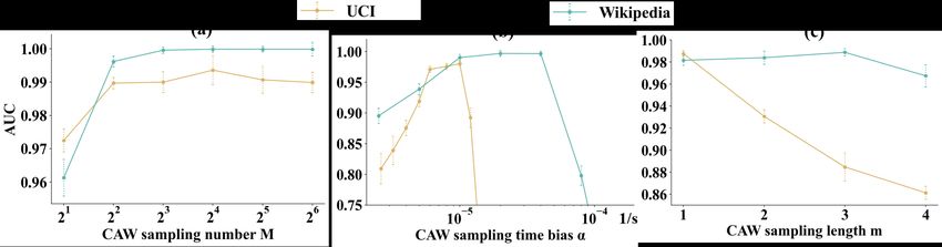
Under review as a conference paper at ICLR 2021

 No. Ablation Wikipedia UCI Social Evo.
 1. original method (CAW-N-mean) 98.49 ± 0.38 99.12 ± 0.33 94.54 ± 0.69
 2. remove f1 (ICAW ) 96.28 ± 0.66 79.45 ± 0.71 53.69 ± 0.21
 3. remove f2 (t) 97.99 ± 0.13 95.00 ± 0.42 71.93 ± 2.32
 4. remove f1 (ICAW ), f2 (t) 88.94 ± 0.85 50.01 ± 0.02 50.00 ± 0.00
 5. replace f1 (ICAW ) by one-hot(IAW ) 96.55 ± 0.21 85.59 ± 0.34 68.47 ± 0.86
 6. fix α = 0 75.10 ± 3.12 87.13 ± 0.49 78.01 ± 0.69
 Table 3: Ablation study with CAW-N-mean. AUC scores on all inductive test links are reported.

 Figure 5: Hyperparameter sensitivity in CAW sampling. AUC on all inductive test links are reported.

scores on Reddit and Wikpedia when the baselines are far from perfect. Meanwhile, the strongest
baseline on these two attributed datasets, TGAT (Xu et al., 2020), suffers a lot on all the other datasets
where informative node / link attributes become unavailable.
Comparing the two training settings, we observe that the performance of four baselines (JODIE,
VGRNN, DynAERNN,DyRep) drop significantly when transiting from the transductive setting to the
inductive one, as they mostly record node identities either explicitly (JODIE, VGRNN, DynAERNN)
or implicitly (DyRep). TGAT and EvolveGCN do not use node identities and thus their performance
gaps between the two settings are small, while they sometimes do not perform well in the transductive
setting, as they encounter the ambiguity issue in Fig. 3. In contrast, our methods perform well
in both the transductive and inductive settings. We attribute this superiority to the anonymization
procedure: the set-based relative node identities well capture the correlation between walks to make
good prediction while removing the original node identities to keep entirely inductive. Even when the
network structures greatly change and new nodes come in as long as the network evolves according to
the same law as the network used for training, CAW-N will always work. Comparing CAW-N-mean
and CAW-N-attn, we see that our attention-based variant outperforms the mean-pooling variant, albeit
at the cost of high computation complexity. Also note that the strongest baselines on all datasets
are stream-based methods, which indicates that the aggregation of links into network snapshots may
remove some useful time information (see more discussion in Appendix D.2).
We further conduct ablation studies on Wikipedia (attributed), UCI (non-attributed), and Social
Evolution (non-attributed), to validate effectiveness of critical components of our model. Tab. 3
shows the results. By comparing Ab.1 with Ab.2, 3 and 4 respectively, we observe that our proposed
node anonymization and encoding, f1 (ICAW ), contributes most to the performance, though the time
encoding f2 (t) also helps. Comparing performance across different datasets, we see that the impact
of ablation is more prominent when informative node/link attributes are unavailable such as with UCI
and Social Evolution. Therefore, in such scenarios our CAWs are highly crucial. In Ab.5, we replace
our proposed ICAW with IAW (Eq.2), which is used in standard AWs, and we use one-hot encoding
of node new identities IAW . We see by comparing Ab.1, 2, and 5 that such anonymization process is
significantly less effective than our ICAW , though it helps to some extent. Finally, Ab.6 suggests that
entirely uniform sampling of the history may hurt performance.

5.3 H YPERPARAMETER I NVESTIGATION OF CAW S AMPLING
We systematically analyze the effect of hyperparameters used in CAW sampling schemes, including
sampling number M , temporal decay coefficient α and walk length m. The experiments are conducted
on UCI and Wikipedia datasets using CAW-N-mean. When investigating each hyperparameter, we
set the rest two to an optimal value found by grid search, and report the mean AUC performance on
all inductive test links (i.e. old vs. new, new vs. new) and their 95% confidence intervals.
The results are summarized in Fig.5. From (a), we observe that only a small number of sampled CAWs
are needed to achieve a competitive performance. Meanwhile, the performance gain is saturated as
the sampling number increases. We can obtain many insights by analyzing the temporal decay α in
(b): α usually has an optimal interval, whose values and length also vary with different datasets to

 8

Under review as a conference paper at ICLR 2021

Figure 6: Complexity evaluation: The accumulated runtime of (a) temporal random walk extraction (Alg.1) and
(b) the entire CAW-N training, timed over one epoch on Wikipedia (using different |E| for training).
capture the different levels of temporal dynamics; a small α suggests an almost uniform sampling of
interaction history, which hurts the performance; meanwhile, an overly large α would damage the
model, since it makes the model only sample the most recent few interactions for computation and
blind to the rest. Based on our efficient sampling strategy (Sec.4.4), we may combine the optimal
α with the average link intensity τ (Tab.1), and concludes that CAW-N only needs to online record
and sample from about a constant times about 5 (≈ ατ ) most recent links for each node. Finally, the
plot (c) suggests that the performance may peak at a certain CAW length, while the exact value may
vary with datasets. Longer CAWs indicate that the corresponding networks evolve according to more
complicated laws that are encoded in higher-order network motifs.
5.4 C OMPLEXITY E VALUATION
Here, we examine how the runtime of CAW-N depends on the number of edges |E| that are used
for training. We record the runtimes of CAW-N for training one epoch on the Wikipedia datasets
using M = 32, m = 2 with batch-size=32. Specifics of the computing infrastructure are given in
Appendix C.5. Fig. 6 (a) shows the accumulated runtime of executing the random walk extraction
i.e. Alg.1 only. It well aligns with our theoretical analysis (Thm. A.2) that each step of the random
walk extraction has constant complexity (i.e. accumulated runtime linear with |E|). Plot (b) shows
the entire runtime for one-epoch training, which is also linear with |E|. Note that O(|E|) is the time
complexity that one at least needs to pay. This study demonstrates our method’s advantage of being
scalable to process long edge streams. NEW

6 C ONCLUSION
We proposed CAW-N to inductively represent the dynamics of temporal networks. CAW-N uses
CAWs to implicitly extract network motifs via temporal random walks and adopts novel set-based
anonymization to establish the correlation between network motifs. The success of CAW-N points
out many promising future research directions on temporal networks: Pairing CAW-N with neural
network interpretation techniques (Montavon et al., 2018) may give a chance to automatically discover
larger and meaningful motifs/patterns of temporal networks; CAW-N may also be generalized to
predict high-order structures (e.g., triangles) that correspond to some function units of temporal
networks from different domains (Benson et al., 2016; 2018; Zitnik et al., 2019). NEW

R EFERENCES
Ghadeer AbuOda, Gianmarco De Francisci Morales, and Ashraf Aboulnaga. Link prediction via
 higher-order motif features. In Joint European Conference on Machine Learning and Knowledge
 Discovery in Databases. Springer, 2019.
Nesreen K Ahmed, Jennifer Neville, Ryan A Rossi, and Nick Duffield. Efficient graphlet counting
 for large networks. In International Conference on Data Mining. IEEE, 2015.
Peter W Battaglia, Jessica B Hamrick, Victor Bapst, Alvaro Sanchez-Gonzalez, Vinicius Zambaldi,
 Mateusz Malinowski, Andrea Tacchetti, David Raposo, Adam Santoro, Ryan Faulkner, et al.
 Relational inductive biases, deep learning, and graph networks. arXiv preprint arXiv:1806.01261,
 2018.
Austin R Benson, David F Gleich, and Jure Leskovec. Higher-order organization of complex networks.
 Science, 353(6295), 2016.

 9

Under review as a conference paper at ICLR 2021

Austin R Benson, Rediet Abebe, Michael T Schaub, Ali Jadbabaie, and Jon Kleinberg. Simplicial
 closure and higher-order link prediction. Proceedings of the National Academy of Sciences, 115
 (48):E11221–E11230, 2018.
Salomon Bochner. A theorem on Fourier-Stieltjes integrals. Collected Papers of Salomon Bochner, 2,
 1992.
Jinyin Chen, Jian Zhang, Xuanheng Xu, Chenbo Fu, Dan Zhang, Qingpeng Zhang, and Qi Xuan.
 E-lstm-d: A deep learning framework for dynamic network link prediction. IEEE Transactions on
 Systems, Man, and Cybernetics: Systems, 2019.
Lun Du, Yun Wang, Guojie Song, Zhicong Lu, and Junshan Wang. Dynamic network embedding:
 An extended approach for skip-gram based network embedding. In International Joint Conference
 on Artificial Intelligence, 2018.
Thomas E Gorochowski, Claire S Grierson, and Mario di Bernardo. Organization of feed-forward
 loop motifs reveals architectural principles in natural and engineered networks. Science advances,
 4(3), 2018.
Palash Goyal, Sujit Rokka Chhetri, and Arquimedes Canedo. dyngraph2vec: Capturing network
 dynamics using dynamic graph representation learning. Knowledge-Based Systems, 187, 2020.
Mark S Granovetter. The strength of weak ties. American journal of sociology, 78(6), 1973.
Ehsan Hajiramezanali, Arman Hasanzadeh, Krishna Narayanan, Nick Duffield, Mingyuan Zhou, and
 Xiaoning Qian. Variational graph recurrent neural networks. In Advances in Neural Information
 Processing Systems, 2019.
Will Hamilton, Zhitao Ying, and Jure Leskovec. Inductive representation learning on large graphs. In
 Advances in Neural Information Processing Systems, 2017a.
William L Hamilton, Rex Ying, and Jure Leskovec. Representation learning on graphs: Methods and
 applications. IEEE Data Engineering Bulletin, 40(3), 2017b.
Petter Holme and Jari Saramäki. Temporal networks. Physics reports, 519(3), 2012.
Sergey Ivanov and Evgeny Burnaev. Anonymous walk embeddings. In International Conference on
 Machine Learning, 2018.
Seyed Mehran Kazemi, Rishab Goel, Sepehr Eghbali, Janahan Ramanan, Jaspreet Sahota, Sanjay
 Thakur, Stella Wu, Cathal Smyth, Pascal Poupart, and Marcus Brubaker. Time2vec: Learning a
 vector representation of time. arXiv preprint arXiv:1907.05321, 2019.
Thomas N Kipf and Max Welling. Variational graph auto-encoders. arXiv preprint arXiv:1611.07308,
 2016.
Thomas N Kipf and Max Welling. Semi-supervised classification with graph convolutional networks.
 In International Conference on Learning Representations, 2017.
Lauri Kovanen, Márton Karsai, Kimmo Kaski, János Kertész, and Jari Saramäki. Temporal motifs in
 time-dependent networks. Journal of Statistical Mechanics: Theory and Experiment, 2011(11),
 2011.
Lauri Kovanen, Kimmo Kaski, János Kertész, and Jari Saramäki. Temporal motifs reveal homophily,
 gender-specific patterns, and group talk in call sequences. Proceedings of the National Academy of
 Sciences, 110(45), 2013.
Srijan Kumar, Xikun Zhang, and Jure Leskovec. Predicting dynamic embedding trajectory in temporal
 interaction networks. In International Conference on Knowledge Discovery Data Mining, 2019.
Mayank Lahiri and Tanya Y Berger-Wolf. Structure prediction in temporal networks using frequent
 subgraphs. In IEEE Symposium on Computational Intelligence and Data Mining, 2007.
Günter Last and Mathew Penrose. Lectures on the Poisson process, volume 7. Cambridge University
 Press, 2017.

 10

Under review as a conference paper at ICLR 2021

Stephen Lavenberg. Computer performance modeling handbook. Elsevier, 1983.
Pan Li and Olgica Milenkovic. Inhomogeneous hypergraph clustering with applications. In Advances
 in Neural Information Processing Systems, 2017.
Taisong Li, Jiawei Zhang, S Yu Philip, Yan Zhang, and Yonghong Yan. Deep dynamic network
 embedding for link prediction. IEEE Access, 6, 2018.
Sedigheh Mahdavi, Shima Khoshraftar, and Aijun An. dynnode2vec: Scalable dynamic network
 embedding. In International Conference on Big Data (Big Data). IEEE, 2018.
Franco Manessi, Alessandro Rozza, and Mario Manzo. Dynamic graph convolutional networks.
 Pattern Recognition, 97, 2020.
Shmoolik Mangan and Uri Alon. Structure and function of the feed-forward loop network motif.
 Proceedings of the National Academy of Sciences, 100(21), 2003.
Silvio Micali and Zeyuan Allen Zhu. Reconstructing markov processes from independent and
 anonymous experiments. Discrete Applied Mathematics, 200, 2016.
Grégoire Montavon, Wojciech Samek, and Klaus-Robert Müller. Methods for interpreting and
 understanding deep neural networks. Digital Signal Processing, 73:1–15, 2018.
Giang Hoang Nguyen, John Boaz Lee, Ryan A Rossi, Nesreen K Ahmed, Eunyee Koh, and Sungchul
 Kim. Continuous-time dynamic network embeddings. In Companion Proceedings of the The Web
 Conference, 2018.
Ashwin Paranjape, Austin R Benson, and Jure Leskovec. Motifs in temporal networks. In Interna-
 tional Conference on Web Search and Data Mining, 2017.
Aldo Pareja, Giacomo Domeniconi, Jie Chen, Tengfei Ma, Toyotaro Suzumura, Hiroki Kanezashi,
 Tim Kaler, Tao B Schardl, and Charles E Leiserson. EvolveGCN: Evolving graph convolutional
 networks for dynamic graphs. In AAAI Conference on Artificial Intelligence, 2020.
Mahmudur Rahman and Mohammad Al Hasan. Link prediction in dynamic networks using graphlet.
 In Joint European Conference on Machine Learning and Knowledge Discovery in Databases.
 Springer, 2016.
Ryan A Rossi, Anup Rao, Sungchul Kim, Eunyee Koh, Nesreen K Ahmed, and Gang Wu. Higher-
 order ranking and link prediction: From closing triangles to closing higher-order motifs. arXiv
 preprint arXiv:1906.05059, 2019.
David E Rumelhart, Geoffrey E Hinton, and Ronald J Williams. Learning representations by
 back-propagating errors. nature, 323(6088), 1986.
Aravind Sankar, Yanhong Wu, Liang Gou, Wei Zhang, and Hao Yang. DySAT: Deep neural
 representation learning on dynamic graphs via self-attention networks. In International Conference
 on Web Search and Data Mining, 2020.
Purnamrita Sarkar, Deepayan Chakrabarti, and Michael I Jordan. Nonparametric link prediction in
 dynamic networks. In International Conference on Machine Learning, 2012.
Franco Scarselli, Marco Gori, Ah Chung Tsoi, Markus Hagenbuchner, and Gabriele Monfardini. The
 graph neural network model. IEEE Transactions on Neural Networks, 20(1), 2008.
Georg Simmel. The sociology of georg simmel, volume 92892. Simon and Schuster, 1950.
Uriel Singer, Ido Guy, and Kira Radinsky. Node embedding over temporal graphs. In International
 Joint Conference on Artificial Intelligence, 2019.
Riitta Toivonen, Jussi M Kumpula, Jari Saramäki, Jukka-Pekka Onnela, János Kertész, and Kimmo
 Kaski. The role of edge weights in social networks: modelling structure and dynamics. In Noise
 and Stochastics in Complex Systems and Finance, volume 6601. International Society for Optics
 and Photonics, 2007.

 11

Under review as a conference paper at ICLR 2021

Rakshit Trivedi, Hanjun Dai, Yichen Wang, and Le Song. Know-evolve: deep temporal reasoning for
 dynamic knowledge graphs. In International Conference on Machine Learning, 2017.
Rakshit Trivedi, Mehrdad Farajtabar, Prasenjeet Biswal, and Hongyuan Zha. Dyrep: Learning
 representations over dynamic graphs. In International Conference on Learning Representation,
 2019.
Ashish Vaswani, Noam Shazeer, Niki Parmar, Jakob Uszkoreit, Llion Jones, Aidan N Gomez, Łukasz
 Kaiser, and Illia Polosukhin. Attention is all you need. In Advances in Neural Information
 Processing Systems, 2017.
Petar Veličković, Guillem Cucurull, Arantxa Casanova, Adriana Romero, Pietro Liò, and Yoshua
 Bengio. Graph attention networks. In International Conference on Learning Representations,
 2018.
Yanbang Wang, Pan Li, Chongyang Bai, VS Subrahmanian, and Jure Leskovec. Generic representa-
 tion learning for dynamic social interaction. International Conference on Knowledge Discovery
 Data Mining, MLG workshop, 2020.
Da Xu, Chuanwei Ruan, Evren Korpeoglu, Sushant Kumar, and Kannan Achan. Self-attention with
 functional time representation learning. In Advances in Neural Information Processing Systems,
 2019.
Da Xu, Chuanwei Ruan, Evren Korpeoglu, Sushant Kumar, and Kannan Achan. Inductive repre-
 sentation learning on temporal graphs. In International Conference on Learning Representation,
 2020.
Le-kui Zhou, Yang Yang, Xiang Ren, Fei Wu, and Yueting Zhuang. Dynamic network embedding by
 modeling triadic closure process. In AAAI Conference on Artificial Intelligence, 2018.
Marinka Zitnik, Marcus W Feldman, Jure Leskovec, et al. Evolution of resilience in protein
 interactomes across the tree of life. Proceedings of the National Academy of Sciences, 116(10),
 2019.

 12

Under review as a conference paper at ICLR 2021

 A E FFICIENT LINK S AMPLING
 Our efficient link sampling strategy contains two subroutines – Online probability computation (Alg.2)
 and Iterative sampling (Alg.3). The Online probability computation subroutine Alg.2 essentially
 works online to assign each new incoming link ({u, v}, t) with a pair of probabilities {pu,t , pv,t }
 such that
 exp(αt) exp(αt)
 pu,t = P 0
 , pv,t = P 0
 . (9)
 (e,t0 )∈Eu,t exp(αt ) (e,t0 )∈Ev,t exp(αt )
 These probabilities will be used later in sampling (Alg.3) and do not need to be updated any more.

 Algorithm 2: Online probability computation (G, α)
1 Initialize V ← ∅, Ω ← ∅;
2 for ({u, v}, t) ∈ E do
 3 for w ∈ {u, v} do
 4 if w 6∈ V then
 5 V ← V ∪ {w};
 6 Pw ← exp(αt);
 7 else
 8 Find Pw ∈ Ω;
 9 Pw ← Pw + exp(αt);
10 pw,t ← exp(αt)
 Pw ;
11 Ω ← Ω ∪ {Pw };
12 Assign two probability scores: ({(u, pu,t ), (v, pv,t )}, t, ) ← ({u, v}, t) ;

 The Iterative sampling subroutine Alg.3 is an efficient implementation of step 5 in Alg.1. We may
 first show that the sampling probability of a link (e, t) in Ewp ,tp is proportional to exp(α(t − tp )) in
 Prop.A.1.

 Algorithm 3: Iterative Sampling (E, α, wp , tp )
1 Initialize V ← ∅, Ω ← ∅;
2 for (e, t) ∈ Ewp ,tp with an decreasing order of t do
 3 Sample a ∼ Unif[0, 1];
 4 pwp ,t is the score of this link related to wp obtained from Alg.2;
 5 if a < pwp ,t then
 6 Return (e, t);
7 Return ({wp , X}, tX );

 Proposition A.1. Based on the probabilities (Eq.9) pre-computed by Alg.2, Alg.3 will sample a link
 (e, t) in Ewp ,tp with probability proportional to exp(α(t − tp )).

 Proof. To show this, we first order the timestamps of links in Ewp ,tp between [t, tp ) as t = t00 < t01 <
 t02 < · · · < t0k < tp where there exists an link (e0 , t0i ) ∈ Ewp ,tp for t0i . Then, the probability to sample
 a link (e, t) ∈ Ewp ,tp satisfies
 k
 Y 

 p = pwp ,t × 1 − pwp ,t0i
 i=1
 exp(αt0 )
 P
 k (e0 ,t0 )∈Ewp ,t0
 exp(αt) Y i−1
 = 0
 ×
 exp(αt0 )
 P P
 (e0 ,t0 )∈Ewp ,t exp (αt ) i=1 (e0 ,t0 )∈E 0
 wp ,t
 i

 exp(αt) exp(α(t − tp ))
 =P 0)
 =P 0
 ,
 (e0 ,t0 )∈Ewp ,tp exp (αt (e0 ,t0 )∈Ewp ,tp exp (α(t − tp ))

 13

Under review as a conference paper at ICLR 2021

which is exactly the probability that we need.

We have the following Thm.A.2 with a weak assumption that evaluates the complexity of Alg.3. We
assume that links come in by following a Poisson point process with intensity τ , which is a frequently
used assumption to model communication networks (Lavenberg, 1983). This result indicates that
if α > 0, for each node, we only need to record the most recent O( ατ ) links to sample. This result
is important as it means our method can do online training and inference with time and memory
complexity that are not related to the total number of links.
Theorem A.2. If the links that are connected to wp appear by following a Poisson point process with
intensity τ . Then, the expected number of iterations of Alg.3 is bounded by min{ 2τα + 1, |Ewp ,tp |}.

Proof. The number of iterations of Alg.3 is always bounded by |Ewp ,tp |. So we only need to prove
that the expected number of interactions of Alg.3 is bounded by 2τ
 α + 1.
To show this, we order the timestamps of links in Ewp ,tp between [0, tp ) as 0 = t0 < t1 < t2 <
· · · < tk < tp where there exists an link (e, ti ) ∈ Ewp ,tp for ti . Further define we define Zi =
exp(α(ti − ti−1 )) for i ∈ [1, k].
Due to the definition of Poisson process, we know that each time difference in {ti − ti−1 }1≤i≤k
follows i.i.d. exponential distribution with parameter τ . Therefore, {Zi }1≤i≤k are also i.i.d.. Let
ψ = E(Zi−1 ) = α+τ τ
 .
The probability that Alg.3 runs j iterations is equal to the probability that the link with timestamp
tk+1−j ) gets sampled. That is
 Qk+1−j
 Zi
 P(iter = j) = Pk i=1 Qk+1−h .
 h=1 i=1 Zi

Therefore, the expected number of iterations is
 " Pk Qk+1−j # k
 " Qj−1 0 #
 j=1 j i=1 Zi i=1 Zi
 X
 E(iter) = E Pk Qk+1−h = jE Pk Qh−1 . (10)
 Zi 0
 h=1 i=1 j=1 h=1 i=1 Zi
 −1 Q0
where Zi0 = Zk+1−i and i=1 Zi0 = 1. Next we will prove that each item in right-hand-side of Eq.10
satisfies
 " Qj−1 0 #
 i=1 Zi
 jE Pk Qh−1 ≤ [1 + (j − 1)(1 − ψ)]ψ j−1 . (11)
 0
 h=1 i=1 Zi
If this is true, then
 k
 X k
 X k
 X
 E(iter) ≤ [1 + (j − 1)(1 − ψ)]ψ j−1 = ψ j−1 + (j − 1)(1 − ψ)ψ j−1
 j=1 j=1 j=1
 1 ψ 2τ
 ≤ + = + 1.
 1−ψ 1−ψ α

Now, let us prove Eq.11. For j = 1, Eq.11 is trivial. For j > 1,
 " Qj−1 0 # " Qj−1 0 # Qj−1 0
 i=1 Zi i=1 Zi i=1 E(Zi ) ψ j−1
 E Pk Qh−1 ≤E j h−1
 ≤ j h−1
 = Pj−1 ,
 0 1 + h=2 i=1 Zi0 1 + h=2 i=1 E(Zi0 ) i
 P Q P Q
 h=1 i=1 Zi i=0 ψ
 (12)
where the second inequality is due to the Jensen’s inequality and the fact that for any positive c1 , c2 ,
 x
c1 +c2 x is concave with respect to x. Moreover, we also have
 j−1
 X j−1
 X
 i
 [1 + (j − 1)(1 − ψ)] ψ =j+ ψ i − (j − 1)ψ j ≥ j. (13)
 i=0 i=1
Combining Eq.12 and Eq.13, we prove Eq.11, which concludes the proof.

 14

Under review as a conference paper at ICLR 2021

B T REE - STRUCTURED SAMPLING
We may further decrease the sampling complexity by revising Alg. 1 into tree-structured sampling.
Alg. 1 originally requires to sample link M m times because we need to search M links that connected
to w0 in the first step and then sample one link for each of the M nodes in each following step. A
tree-structured sampling strategy Qmay reduce this number: Specifically, we sample ki links for each
 m
node in step i but we make sure i=1 ki = M , which Pm does not change the total number of walks.
In this way, the times of link search decrease to i=1 k1 k2 ...ki . Suppose M = 64, m = 3, and
k1 = 4, k2 = 4, k3 = 4, then the times of link search decrease to about 0.44M m . Though empirical
results below show that tree-structured sampling achieves slightly worse performance, it provides an
opportunity to tradeoff between prediction performance and time complexity.

 Figure 7: Effect of sampling of different tree structures on inductive performance.
We conduct more experiment to investigate this topic with Wikipedia and UCI datasets. The setup is
as follows: first, we fix CAW sampling number M = 64 = 26 and length m = 2, so that we always
have k1 k2 = M = 26 ; next, we assign different values to k1 , so that the shape of the tree changes
accordingly; controlling other hyperparameters to be the optimal combination found by grid search,
we plot the corresponding inductive AUC scores of CAW-N-mean on all testing edges in Fig. 7. It is
observed that while tree-structured sampling may affect the performance to some extent, its negative
impact is less prominent when the first-step sampling number k1 is relatively large, and our model
still achieves state-of-the-art performance compared to our baselines. That makes the tree-structured
sampling a reasonable strategy that can further reduce time complexity.

C A DDITIONAL E XPERIMENTAL S ETUP D ETAILS
C.1 DATASET I NTRODUCTION AND ACCESS

We list the introduction of the six datasets as follows.

 • Reddit1 is a dataset of posts made by users on subredditts over a month. Its nodes are users
 and posts, and its links are the timestamped posting requests.
 • Wikipedia2 is a dataset of edits over wiki pages over a month, whose nodes represent human
 editors and wiki pages and whose links represent timestamped edits.
 • Social Evolution3 is a dataset recording the detailed evolving physical proximity between
 students in a dormitory over a year, deterimined from wireless signals of their mobile
 devices.
 • Enron4 is a communication network whose links are email communication between core
 employees of a cooperation over several years.
 • UCI5 is a dataset recording online posts made by university students on a forum, but is
 non-attributed.
 • MOOC6 is a dataset of online courses where nodes represent students and course content
 units such as videos and problem sets, and links represent student’s access behavior to a
 particular unit.
 1
 http://snap.stanford.edu/jodie/reddit.csv
 2
 http://snap.stanford.edu/jodie/wikipedia.csv
 3
 http://realitycommons.media.mit.edu/socialevolution.html
 4
 https://www.cs.cmu.edu/~./enron/
 5
 http://konect.cc/networks/opsahl-ucforum/
 6
 http://snap.stanford.edu/jodie/mooc.csv

 15