Probing dark energy with tomographic weak-lensing aperture mass statistics
←
→
Page content transcription
If your browser does not render page correctly, please read the page content below
A&A 646, A62 (2021)
https://doi.org/10.1051/0004-6361/202039679                                                                                                               Astronomy
c N. Martinet et al. 2021                                                                                                                                  &
                                                                                                                                                          Astrophysics

     Probing dark energy with tomographic weak-lensing aperture
                           mass statistics
                         Nicolas Martinet1 , Joachim Harnois-Déraps2,3 , Eric Jullo1 , and Peter Schneider4

      1
          Aix-Marseille Univ, CNRS, CNES, LAM, Marseille, France
          e-mail: nicolas.martinet@lam.fr
      2
          Institute for Astronomy, University of Edinburgh, Royal Observatory, Blackford Hill, Edinburgh EH9 3HJ, UK
      3
          Astrophysics Research Institute, Liverpool John Moores University, 146 Brownlow Hill, Liverpool L3 5RF, UK
      4
          Argelander-Institut für Astronomie, Universität Bonn, Auf dem Hügel 71, 53121 Bonn, Germany
     Received 14 October 2020 / Accepted 20 November 2020

                                                                                     ABSTRACT

     We forecast and optimize the cosmological power of various weak-lensing aperture mass (Map ) map statistics for future cosmic shear
     surveys, including peaks, voids, and the full distribution of pixels (1D Map ). These alternative methods probe the non-Gaussian regime
     of the matter distribution, adding complementary cosmological information to the classical two-point estimators. Based on the SLICS
     and cosmo-SLICS N-body simulations, we build Euclid-like mocks to explore the S 8 − Ωm − w0 parameter space. We develop a
     new tomographic formalism that exploits the cross-information between redshift slices (cross-Map ) in addition to the information
     from individual slices (auto-Map ) probed in the standard approach. Our auto-Map forecast precision is in good agreement with the
     recent literature on weak-lensing peak statistics and is improved by ∼50% when including cross-Map . It is further boosted by the use
     of 1D Map that outperforms all other estimators, including the shear two-point correlation function (γ-2PCF). When considering all
     tomographic terms, our uncertainty range on the structure growth parameter S 8 is enhanced by ∼45% (almost twice better) when
     combining 1D Map and the γ-2PCF compared to the γ-2PCF alone. We additionally measure the first combined forecasts on the
     dark energy equation of state w0 , finding a factor of three reduction in the statistical error compared to the γ-2PCF alone. This
     demonstrates that the complementary cosmological information explored by non-Gaussian Map map statistics not only offers the
     potential to improve the constraints on the recent σ8 –Ωm tension, but also constitutes an avenue to understanding the accelerated
     expansion of our Universe.
     Key words. gravitational lensing: weak – cosmology: observations – dark energy – large-scale structure of Universe – surveys

1. Introduction                                                                                  2015; Barthelemy et al. 2020). Two-point statistics fail to cap-
                                                                                                 ture this non-Gaussian information and thus yield an incomplete
The coherent distortion between galaxy shapes due to the gravi-                                  description of the matter distribution at low redshift. To close this
tational lensing by large-scale structure has emerged as one of                                  gap, the community has recently started to explore non-Gaussian
the most powerful cosmological probes today. So-called cos-                                      cosmic shear estimators: for example weak-lensing peaks (e.g.,
mic shear analyses have started to unlock their potential thanks                                 Kruse & Schneider 1999, 2000; Dietrich & Hartlap 2010; Kra-
to large observational surveys of hundreds of square degrees at                                  tochvil et al. 2010; Fan et al. 2010; Yang et al. 2011; Maturi et al.
optical wavelength: for example, CFHTLenS (Heymans et al.                                        2011; Hamana et al. 2012; Hilbert et al. 2012; Marian et al. 2012,
2012), KiDS (de Jong et al. 2013), DES (Flaugher 2005), and                                      2013; Shan et al. 2014, 2018; Lin & Kilbinger 2015; Martinet
HSC (Aihara et al. 2018). In the meantime, the community is                                      et al. 2015, 2018; Liu et al. 2015a,b; Kacprzak et al. 2016; Petri
preparing for the next generation of cosmic shear surveys that                                   et al. 2016; Zorrilla Matilla et al. 2016; Giocoli et al. 2018; Peel
will probe thousands of square degrees and extend to large red-                                  et al. 2018; Davies et al. 2019; Fong et al. 2019; Li et al. 2019;
shifts: for example, Euclid (Laureijs et al. 2011), Vera C. Rubin                                Weiss et al. 2019; Yuan et al. 2019; Coulton et al. 2020; Ajani
Observatory (formerly LSST, Ivezić et al. 2019), and Nancy                                      et al. 2020; Zürcher et al. 2021), Minkowski functionals (e.g.,
Grace Roman Space Telescope (formerly WFIRST, Spergel                                            Kratochvil et al. 2012; Petri et al. 2015; Vicinanza et al. 2019;
et al. 2015).                                                                                    Parroni et al. 2020; Zürcher et al. 2021), higher-order moments
    So far, these surveys have mostly relied on two-point esti-                                  (e.g., Van Waerbeke et al. 2013; Petri et al. 2015; Peel et al. 2018;
mators for their cosmological analysis, for example the shear                                    Vicinanza et al. 2018; Chang et al. 2018; Gatti et al. 2020), three-
two-point correlation functions (γ-2PCF, e.g., Kilbinger et al.                                  point statistics (e.g., Schneider & Lombardi 2003; Takada & Jain
2013; Troxel et al. 2018; Hikage et al. 2019; Asgari et al. 2021).                               2003, 2004; Semboloni et al. 2011; Fu et al. 2014), density split
These estimators are inherited from cosmic microwave back-                                       statistics (e.g., Friedrich et al. 2018; Gruen et al. 2018; Burger
ground (CMB) analyses, which probe the matter distribution of                                    et al. 2020), persistent homology (e.g., Heydenreich et al. 2021),
the early Universe. However, cosmic shear probes the recent                                      scattering transform (e.g., Cheng et al. 2020), and machine learn-
Universe, where the matter distribution is more complex due to                                   ing (e.g., Merten et al. 2019; Ribli et al. 2019; Peel et al. 2019;
the nonlinear accretion of structures that creates non-Gaussian                                  Shirasaki et al. 2019; Fluri et al. 2019). Although these new
features in the matter field on small scales (e.g., Codis et al.                                 statistics have shown a great potential, they have not yet been

                                                                                                                                                                             A62, page 1 of 16

                Open Access article, published by EDP Sciences, under the terms of the Creative Commons Attribution License (https://creativecommons.org/licenses/by/4.0),
                                 which permits unrestricted use, distribution, and reproduction in any medium, provided the original work is properly cited.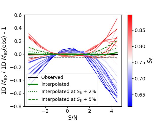
A&A 646, A62 (2021)

fully generalized to data analyses, mostly because they need a            text of a joint analysis with standard two-point estimators. We
large number of computationally expensive N-body simulations              finally test the impact of performing the Map map computation
to calibrate their dependence on cosmology, while this depen-             in real or Fourier space, in presence of observational masks, and
dence is accurately predicted by theoretical models in the case           study the effect of parameter sampling explored with the N-body
of two-point estimators.                                                  simulations.
     In particular, weak-lensing peak statistics have proven to be            The covariance matrix is built from the SLICS simulations
one of the most powerful such new probes. Recent observation-             (Harnois-Déraps et al. 2015) while the cosmology dependence
(e.g., Liu et al. 2015a; Kacprzak et al. 2016; Martinet et al.            is modeled with the cosmo-SLICS (Harnois-Déraps et al. 2019),
2018) and simulation-based (e.g., Zürcher et al. 2021) anal-              which sample the parameters S 8 , Ωm , w0 and the reduced Hubble
yses show that peak statistics improve the constraints on                 parameter h at 25 points. This allows us to model the signals
S 8 = σ8 (Ωm /0.3)0.5 by 20% to 40% compared to the γ-2PCF                everywhere inside a broad parameter space and therefore to sur-
alone. This particular combination of the matter density Ωm and           pass the Fisher analyses often performed in the literature.
clustering amplitude σ8 runs across the main degeneracy direc-                We first describe the mass map calculation that we use (Map )
tion obtained from cosmic shear constraints. It has notably been          in Sect. 2, and investigate its sensitivity to observational masks in
used to assess the potential tension between KiDS γ-2PCF cosmic
                                                                          Appendix A. We then present in Sect. 3 the SLICS and cosmo-
shear and Planck CMB analyses (e.g., Hildebrandt et al. 2017;
                                                                          SLICS N-body simulation mocks. We detail the different data
Planck Collaboration VI 2020; Joudaki et al. 2020; Heymans
et al. 2021). In this article, we generalize the peak formalism to        vectors (DVs) in Sect. 4 and our new tomographic approach in
aperture-mass statistics, which provides additional constraining          Sect. 5. We present the likelihood pipeline used to make our
power on S 8 .                                                            cosmological forecasts in Sect. 6, examining the cosmological
     The aperture mass map (Map map in the following) is essen-           parameter sampling in Appendix B. We forecast the constraints
tially a map of convergence, convolved with a “Mexican hat”-              on S 8 and w0 from Map statistics in Sect. 7, focusing on the
like filter, which can be directly obtained from the estimated            tomography improvement (Sect. 7.1) and on the sampling of Map
shear field (see Sect. 2). Other interesting Map map-sampling             (Sect. 7.2), and finally combine it with the γ-2PCF (Sect. 8). We
methods exist beside peaks: for example voids (e.g., Gruen et al.         summarize our results in Sect. 9.
2016; Coulton et al. 2020) and the full distribution of pixels,
also known as the lensing probability distribution function (lens-        2. Aperture mass computation
ing PDF, e.g., Patton et al. 2017; Shirasaki et al. 2019; Liu &
Madhavacheril 2019). Because they probe more massive struc-               The Map statistic, first defined by Schneider (1996), presents sev-
tures, peaks are less sensitive to noise and are likely better for        eral advantages over classical mass reconstructions that particu-
studying cosmological parameters sensitive to matter (Ωm , σ8 )           larly fit the purpose of cosmological analyses from mass maps.
and the sum of neutrino mass (Coulton et al. 2020). Voids, how-           We first describe the general expression for Map in the shear
ever, could offer a better sensitivity to dark energy. The optimal        and convergence space and discuss the pros and cons of this
choice of lensing estimator is currently unknown and needs to be          method (Sect. 2.1). We then develop a Fourier space approach
determined.                                                               that increases the speed of the reconstruction (Sect. 2.2).
     In the context where Stage-IV weak lensing experiments are
about to see first light, one of the key questions that needs to be
                                                                          2.1. Real space computation
addressed is how much improvement can we expect from higher-
order statistics when it comes to constraining the dark energy            The Map at a position θ0 consists in a convolution between the
equation of state w0 . In this paper, we present the first forecasts      tangential ellipticity t (θ, θ0 ) with respect to that point and a cir-
of this parameter from joint Map and γ-2PCF statistics and pro-           cularly symmetrical aperture filter Q(θ) (with θ = |θ|),
vide recommendations for applying tomography in a way that
optimizes the total constraining power.                                                1 X
                                                                          Map (θ0 ) =          Q(|θi − θ0 |)t (θi , θ0 ),                    (1)
     Indeed, while routinely used in γ-2PCF analyses, tomogra-                        ngal i
phy has rarely been applied in mass map cosmological analyses
(e.g., Yang et al. 2011; Martinet et al. 2015; Petri et al. 2016; Li      where the sum is carried out over observed galaxies and normal-
et al. 2019; Coulton et al. 2020; Ajani et al. 2020; Zürcher et al.       ized by the galaxy density ngal within the aperture. The tangential
2021), less so with a realistic redshift distribution (e.g., Martinet     ellipticity is defined from the two components of the ellipticity
et al. 2015; Petri et al. 2016; Zürcher et al. 2021). One caveat of       and the polar angle φ(θ, θ0 ) of the separation vector θ − θ0 with
the current mass map tomography is that it only probes the infor-         respect to the center of the aperture θ0 ,
mation from individual redshift slices. This is similar to using                           h                  i
only the auto-correlation terms in the case of the γ-2PCF and             t (θ, θ0 ) = −< ˆ (θ) e−2iφ(θ,θ0 ) .                         (2)
likely explains why the γ-2PCF benefits more from tomography
than mass map estimators (Zürcher et al. 2021). In this article,                A hat denotes spin-2 quantities. Assuming that the mean
we develop a new mass map tomographic approach to include                 intrinsic ellipticity within the aperture averages to 0, Eq. (1)
the cross-information between redshift slices, and apply it to            is an unbiased estimator of Eq. (3) in the weak-lensing regime
simulated lensing catalogs matched in depth to the future Euclid          (|γ̂|, |κ|  1) where the reduced shear ĝ = γ̂/ (1 − κ) is equal to
survey, with a broad redshift distribution between 0 < z < 3.             the shear γ̂:
     The aim of this article is to serve as a basis for the application                 Z
of Map non-Gaussian statistics to future cosmic shear surveys.            Map (θ0 ) =      d2 θ Q(|θ − θ0 |) γt (θ, θ0 ),                  (3)
In particular we review and optimize the statistical precision
gain on S 8 and w0 brought by different samplings of the Map              The tangential shear γt (θ, θ0 ) is computed by replacing ˆ by γ̂ in
map, either using the full distribution of pixels, the peaks, or the      Eq. (2), and is related to the intrinsic galaxy ellipticity ˆS through
voids. We also optimize the tomographic approach in the con-              ˆ = (ˆS + ĝ)/(1 + ĝ∗ ˆS ) (Seitz & Schneider 1997). Throughout
A62, page 2 of 16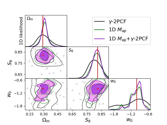
N. Martinet et al.: Probing dark energy with aperture mass statistics
this paper, we use the reduced shear, as this corresponds to the parameter in the NFW profile. The xc θap is referred to as the
quantity observed in data. We also tested our whole pipeline effective size of the aperture, and corresponds to the smoothing
on the shear γ̂ instead and verified that it does not impact our scale of the mass map in other traditional mass reconstruction
cosmological forecasts, validating the use of Map with reduced (e.g., Kaiser & Squires 1993). The first term in Eq. (8) intro-
shear. duces a smooth transition to 0 in the core and edge of the profile.
As demonstrated in Schneider & Bartelmann (1997), the These cuts avoid the singularity in the aperture center, where γt is
aperture mass can equivalently be written as a convolution of not defined, and the contamination from the strong shear regime
the convergence κ(θ) and a compensated aperture filter U(θ): when centered on a massive halo.
Z Following Hetterscheidt et al. (2005), we use xc = 0.15 as an
optimal value for halo detection. Although a particular effective
Map (θ0 ) = d2 θ U(|θ − θ0 |) κ(θ), (4) aperture size increases the S/N of halos with the same physi-
Z ∞ cal scale in the Map map, it also acts as a smoothing for shape
Q(θ0 )
U(θ) = 2 dθ0 − Q(θ). (5) noise and depends on the galaxy density. We tested six differ-
θ θ0 ent effective scales (0.50 , 1.00 , 1.50 , 2.00 , 2.50 , 30 ) and found that
θap xc = 1.50 (corresponding to an aperture size θap = 100 ) maxi-
As U(θ) is a compensated filter, dθ θ U(θ) = 0, which
R
mizes the cosmological forecasts in the case of our mocks in all
means that the residual constant from integrating the shear into
tomographic configurations, and therefore only present results
the convergence vanishes. This is not the case for classical mass for this aperture size. This optimal scale is closely followed by
reconstructions (e.g., Kaiser & Squires 1993) which usually the 10 and 20 scales in term of forecast precision, in good agree-
resort to averaging the mass map to zero to lower the impact ment with other stage IV forecasts (for example Li et al. 2019
of that constant, referred to as mass sheet degeneracy. As the found an optimal smoothing scale of 20 for their LSST mocks).
integration constant will vary from field to field and between The fact that we find the same optimal θap in the different tomo-
the observational data and the modeled ones, it introduces ran- graphic cases suggests that the choice of aperture size is dom-
dom variations to the mass levels that could bias the cosmologi- inated by the scale of the matched structures rather than the
cal constraints from mass map statistics. Dealing with the mass noise smoothing thanks to the high galaxy density. We do not
sheet degeneracy issue makes Map a well suited method for cos- explore the combination of Map statistics measured from multi-
mology analyses (e.g., peak statistics). ple smoothing scales as Martinet et al. (2018) showed that this
Another important advantage of Map is that one can define a combination of scales only marginally improves the cosmologi-
local noise as the dispersion of Map assuming no shear, that is cal constraints in the case of Map map peaks.
only due to galaxy intrinsic ellipticities:
1/2 2.2. Fourier space computation
1 X
σ(Map (θ0 )) = √ |ˆ (θi )| Q (|θi − θ0 |) .
2 2
(6) Aperture masses are conveniently computed in Fourier space,
2ngal i
where the convolution becomes a product:
The σ(Map (θ0 )) accounts for local variations of the galaxy den- h i
ap = −< Q e γ̂ ,
M ] −2iφ e (9)
sity that arise from masks or different magnitude depths within a g
survey.
From Eqs. (1) & (6), one can derive the local signal-to-noise where a tilde denotes Fourier transformed quantities. Carrying
ratio (S/N), which will be used to measure the height of Map out the convolution with FFT significantly reduces the com-
pixels: putational time. In our case, for a 1024 × 1024 pixel map of
√ P 100 deg2 with a galaxy density of 30 arcmin−2 and a filter scale
S 2 Q(|θi − θ0 |)t (θi , θ0 ) of 10 arcmin, the Fourier space approach is ∼25 times faster than
(θ0 ) = pP i . (7) in real space, dropping from ∼50 to ∼2 min on a regular desktop
N (θi )|2 Q2 (|θi − θ0 |)
i |ˆ computer.
In contrast to Martinet et al. (2018), we do not include galaxy Although they are equivalent in theory, the real and Fourier
weights and shear multiplicative biases as this article is primarily space approaches differ in practice: The Fourier approach suf-
intended to assess the potential of Map map cosmology for future fers from a loss of resolution and periodic boundary effects. The
cosmic shear surveys in terms of gain in precision. The impact latter effect is suppressed by removing a stripe of width θap at
the field boundary after the convolution (as is also done in the
of the shear measurement systematics, while being an important
direct-space computation). While we use exact galaxy positions
topic, is beyond the scope of this paper.
in real space, we have to bin them on a map before perform-
The formalism above does not assume any particular func-
ing the Fourier transform, reducing the resolution to that of the
tion for Q(θ) besides the circular symmetry. In this work, we use
final map.
the Schirmer et al. (2007) filter which is a simpler form of an
Despite these limitations, our Fourier-space and real-space
NFW (Navarro et al. 1997) halo mass profile, and is hence opti-
approaches agree very well in the absence of masks, produc-
mized to detect dark matter halos associated with small-scale
ing visually identical maps with a null mean residual per pixel.
structures in Map maps,
Exploring the impact on the distribution of S/N values of the
−1 Map map, we find that the Fourier approach introduces a loss of
Q(θ) = 1 + exp 6 − 150 θθap + exp −47 + 50 θθap power for the high S/N, with 5% fewer pixels with S /N ≥ 3.0
−1 (8) compared to the real-space computation. This power leakage due
× xcθθap tanh xcθθap , to the discretization of galaxy positions in Fourier space depends
on the sampling frequency: it is of 14% if we decrease the pixel
where θap is the size of the aperture and xc indicates a change resolution by a factor two and drops to only 2% if we increase
of slope at the angular scale xc θap and is analogous to the rs the resolution by the same factor (i.e., reconstructing a 512 × 512
A62, page 3 of 16
A&A 646, A62 (2021)

and 2048 × 2048 pixels map respectively). We however keep our         ing the origin2 . A 26th cosmo-SLICS simulation was run with
fiducial resolution (1024 × 1024 pixels) to lower the computa-        the same set-up but with cosmological parameters fixed to the
tional time. We also verified that the Fourier reconstruction does    SLICS ΛCDM model, and is used to mock the observational
not significantly bias the cosmological forecasts. We find almost     data, from which we try to estimate the cosmology.
no difference (below 0.3% on any parameter precision and bias)            The accuracy of the SLICS and cosmo-SLICS N-body sim-
between the forecasts in Fourier and real space, validating the       ulations was quantified with two-point correlation functions and
use of the Fourier approach.                                          power spectra in Harnois-Déraps et al. (2015, 2019), and is basi-
    In the Map formalism, observational masks affect all pixels       cally within 2% of the Cosmic Emulator (Heitmann et al. 2014)
closer to the mask than the aperture size both in the direct and      up to k = 2.0 h Mpc−1 , with a gradual degradation of the accu-
Fourier approaches. It is then mandatory to apply the same mask       racy at smaller scales. The covariance matrix measured from the
to the simulations used to build the cosmology dependence of          SLICS is also in excellent agreement with the analytical predic-
Map . In Appendix A, we investigate the possible impact of a rep-     tions, at least for γ-2PCF and power spectra, and was shown in
resentative Euclid mask on the cosmological forecasts. We find a      Harnois-Déraps et al. (2019) to contain more than 80% of the
decrease in the forecast precision consistent with the loss of area   “super sample covariance”. This is a strong indicator of the high
due to masking and no bias for both the direct- and Fourier-space     accuracy we achieve on the covariance matrix estimated with the
map computations. In the rest of the paper we use the Fourier-        SLICS.
space approach and do not apply any observational mask.
                                                                      3.2. Redshift distribution
3. Building mock catalogs                                             From the shear and convergence planes described in the last
                                                                      section, we then constructed a mock galaxy catalog for each
3.1. SLICS and cosmo-SLICS
                                                                      light-cone. Because the shear and convergence depend both on
The analysis presented in this work relies on two suites of numer-    the foreground mass and the source redshifts, it is mandatory
ical weak lensing simulations, the Scinet LIght Cones Simula-         to reproduce the redshift distribution of the target survey when
tions (SLICS; Harnois-Déraps et al. 2015, 2018) and the cosmo-        building the mocks. In order to mimic a survey at the expected
SLICS (Harnois-Déraps et al. 2019), which are respectively used       depth of the Euclid Wide Survey (Laureijs et al. 2011), we
for estimating the covariance matrix and modeling the signal of       built a representative redshift distribution from the COSMOS
our different statistics. Both are based on a series of 100 deg2      2015 catalog (Laigle et al. 2016) and used a galaxy density of
light-cones extracted from N-body simulations with the multiple       30 arcmin−2 (Laureijs et al. 2011). We first selected COSMOS
plane technique described in the above references. The under-         galaxies with an i0 -band magnitude lower than 24.5 to account
lying gravity-only calculations were carried out by cubep3 m          for the expected limiting magnitude of the Euclid lensing sample
(Harnois-Déraps et al. 2013) and evolve 15363 particles inside a      in the V IS band, a large filter covering the r, i, and z bands. We
box of comoving side set to 505 h−1 Mpc. Multiple mass sheets         then built the distribution of photometric redshifts in the range
were written to disk at regular comoving intervals, and were sub-     0 < z < 3, with a large bin size of 0.1 in redshift in order to
sequently used to generate convergence (κ) and shear (γ1/2 ) maps     smooth the individual structures in the COSMOS field. We fit
for a series of source planes (between 15 and 28, depending on        this redshift distribution with the Fu et al. (2008) function,
the cosmology) from which the lensing quantities can be inter-
                                                                                 za + zab
polated given a position and a redshift.                              n(z) = A            .                                              (10)
    The SLICS were specifically designed for the estimation of                    zb + c
covariance matrices: They consist of 928 fully independent N-         We see in Fig. 1 that this function is able to reproduce the full
body ΛCDM runs in which the cosmological parameters are               redshift distribution, including the high-z tail, and smooths iso-
fixed to Ωm = 0.2905, σ8 = 0.826, h = 0.6898, ns = 0.969 and          lated peaks that are due to cosmic variance. This would not be
Ωb = 0.0473, while the random seeds in the initial conditions         the case for the classical Smail et al. (1994) function, n(z) ∝
are varied, allowing us to estimate covariance matrices with the      (z/z0 )α exp [−(z/z0 )β ], which fails to capture the high-redshift
“brute force” ensemble approach. A single light-cone was con-         tail above z ∼ 2. The parameters of the fit that are used to gener-
structed from each N-body run, ensuring a complete indepen-           ate the redshift distributions in our simulations are: A = 1.7865
dence between the 928 light-cones.                                    arcmin−2 , a = 0.4710, b = 5.1843, and c = 0.7259.
    The cosmo-SLICS were run with a similar but complemen-
tary N-body configuration: The random seeds are fixed, while
the cosmological parameters Ωm , S 8 , h, and w0 are sampled at 25    3.3. Galaxy positions and ellipticities
points1 . The parameters ns and Ωb were fixed to the value used in    Galaxy 2D projected positions are randomly drawn from a uni-
the SLICS. The sampling of this 4D space follows a Latin hyper-       form distribution. The correlation between the density of galax-
cube, which maximizes the interpolation accuracy. Additionally,       ies and matter is therefore not captured in our galaxy mocks.
at each of these nodes, a pair of simulations was produced, in        Since the average value of the lensing estimator is unaffected
which the sampling variance was highly suppressed from a care-        by the source galaxy positioning, this choice does not bias our
ful selection of the initial conditions (see Harnois-Déraps et al.    cosmological predictions. However, when using simulations in
2019) such that any measurement averaged over the pair nearly         combination with observations, the positions of galaxies in the
follows the ensemble mean. In total, ten pseudo-independent           simulations are chosen to mimic that of the observation, so as
light-cones were constructed at every cosmo-SLICS cosmology           to reduce the impact of masks and shape noise. As a side effect,
(five per pair member) by randomly rotating the planes and shift-     this positioning introduces wrong correlations between galaxy
                                                                      positions and matter overdensities in the simulations. This is
1
   The cosmo-SLICS sample S 8 = σ8 (Ωm /0.3)0.5 instead of σ8 since
the former probes the σ8 –Ωm plane perpendicularly to the lensing     2
                                                                         The full suite contains 50 such light-cones, but we verified that our
degeneracy, and is thus best measured by γ-2PCF.                      signal converged on the mean with 10.

A62, page 4 of 16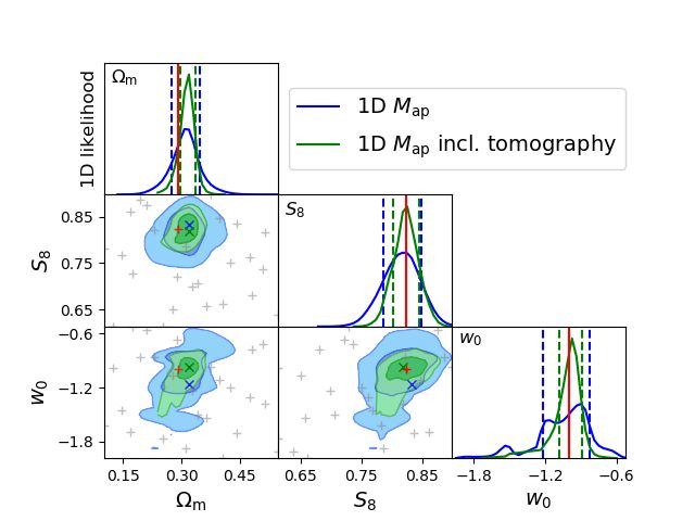
N. Martinet et al.: Probing dark energy with aperture mass statistics
Fig. 1. Redshift distribution normalized to 30 gal.arcmin−2 . The red his- Fig. 2. S/N distribution (or data vectors) of three different Map sam-
togram corresponds to the COSMOS2015 photometric redshift distri- plings: voids (blue), peaks (green), and full 1D distribution (red). Dotted
bution after a cut at i0 ≤ 24.5, the green curve to the fit of a Smail et al. lines correspond to the S/N distributions measured in noise-only maps.
(1994) function to the COSMOS2015 histogram, and the blue curve to Numbers are quoted for a 1024 × 1024 pixels map of 100 deg2 with a
a Fu et al. (2008) fit. In this paper we use the Fu et al. (2008) fit that filter size θap = 100 .
captures the high-redshift tail in contrast to the other function.
often corrected for through the computation of a boost factor resentation of massive halos. Peaks therefore share some infor-
that corresponds to the ratio of the radial number density pro- mation with galaxy cluster counts and both probes aim at explor-
files of galaxies around observed and simulated mass peaks (e.g., ing the non-Gaussian tail of the matter distribution. Peaks, how-
Kacprzak et al. 2016; Shan et al. 2018). Although we can neglect ever, present the advantages of being insensitive to the classical
this effect in simulation-only analyses, a careful measurement of selection function and mass-observable relation issues inherent
this bias will be necessary to unlock the full potential of Map to cluster count studies (e.g., Sartoris et al. 2016; Schrabback
statistics in observational analyses. et al. 2018; Dietrich et al. 2019; McClintock et al. 2019). Min-
When assigning an intrinsic ellipticity ˆS to the mock galax- ima probe the voids of the matter distribution. Alternatively, one
ies, each component is drawn from a Gaussian distribution with can use the full distribution of pixel values (hereafter 1D Map or
zero mean and a dispersion σ = 0.26. This latter value corre- lensing PDF).
sponds to Hubble Space Telescope measurements for galaxies of The number count distribution of these estimators as a func-
magnitudes i ∼ 24.5 (Schrabback et al. 2018), which will consti- tion of S/N constitute our data vectors – DVs for short. They
tute most of the Euclid lensing sample and was used previously are shown in Fig. 2 for a 100 deg2 of mock data without tomo-
to investigate the impact of faint blends on shear estimates (e.g., graphic decomposition. 1D Map is displayed in red, peaks in
Euclid Collaboration 2019). green, and voids in blue. The curves correspond to the mean
Galaxy positions and intrinsic ellipticities constitute the pri- over 50 mock observations from the cosmo-SLICS fiducial cos-
mary source of noise for the extraction of the cosmological sig- mology (2 different initial conditions for the N-body run, five
nal. To prevent any noise effect on the model of the cosmological different ray-tracing through the light-cones, and five different
dependence of the mass map, we fix the positions, redshifts and shape noise realizations) and the error bars are estimated from
intrinsic ellipticities of every galaxy in the cosmo-SLICS mocks the diagonal elements of the covariance matrix computed from
for all the different cosmologies, in which only the cosmic shear the SLICS. As expected from their definition, peaks correspond
is changed. These sources of noise are however included in the to higher S/N pixels while the distribution of voids is centered
covariance matrix: Each mass map is computed from an individ- on lower S/N. The dotted lines in Fig. 2 show the DVs measured
ual realization of the SLICS mocks with different galaxy posi- from noise-only maps computed for the five shape noise real-
tions and ellipticities. See Sect. 6 for more details. izations we use. We see that Map maps are dominated by noise,
with only a small fraction of the DVs carrying the cosmic shear
information. However, the DVs extend to S/N values well above
4. Data vectors that of the noise-only DVs. These broader wings also imply that
In this section we define several estimators built from the Map the DVs are below the noise near their maximum to preserve
maps (Sect. 4.1) as well as the classical γ-2PCF (Sect. 4.2), normalization.
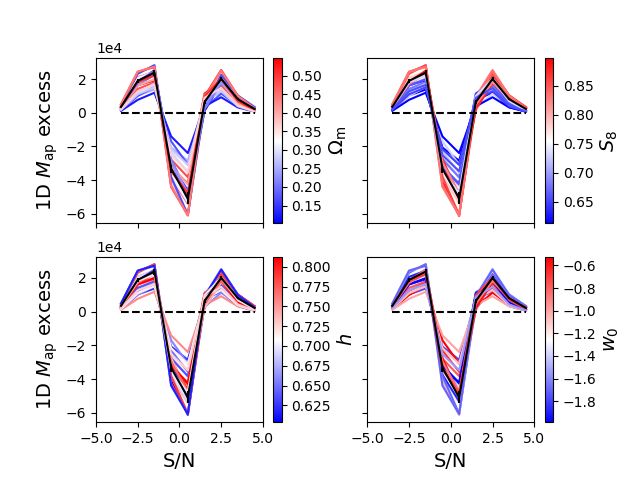
which serves as our baseline comparison method. In Fig. 3, we exhibit the cosmology dependence by compar-
ing 1D Map from Fig. 2 (in black) with that from the cosmo-
SLICS simulations probing a range of cosmological parameters
4.1. Sampling the Map distribution (blue to red curves). As for Fig. 2, we show the mean over 50 Map
Once Map maps have been generated, there are several choices to maps of 100 deg2 each, from which we subtracted the noise
sample the 1D distribution of Map . In this article we investigate contribution to better visualize the cosmology dependence. The
the use of distributions of Map pixels that have larger S/N values dependence on Ωm , S 8 , h, and w0 are shown in different panels
than their n neighboring pixels. In particular, n = 8 corresponds and colored from blue to red for increasing parameter values.
to maxima, and n = 0 to minima. Maxima, or peaks, trace the We find a smooth gradient of 1D Map with S 8 , and a some-
matter overdensities and in the high-S/N regime are a good rep- what smaller variation with Ωm and w0 , highlighting a strong
A62, page 5 of 16A&A 646, A62 (2021)
Fig. 3. Variation of the excess number of Map
pixels over noise with cosmology. The black
curve corresponds to the excess 1D Map in
the observation mock, with error bars from the
diagonal of the covariance matrix. Color-coded
are variations in Ωm (top left), S 8 (top right), h
(bottom left), and w0 (bottom right). A smooth
color gradient indicates a correlation between
the data vector and the probed cosmological
parameter. No tomography has been performed
here.
dependence on these parameters. There however does not seem to build a theoretical model of its cosmology dependence (see
to be any particular dependence on h. e.g., Kilbinger 2015, for a review), we use the cosmo-SLICS
In Fig. 3 and all the following results we consider only the mocks to model the dependence of the γ-2PCF on cosmology.
S/N ranges that can be accurately modeled with our emulator This ensures a fair comparison between the different probes and
(see Sect. 6.3): −2.5 < S /N < 5.5 for peaks, −5 < S /N < 3 also allows for a full combination of DVs when measuring joint
for voids, and −4 < S /N < 5 for 1D Map , and use a bin size constraints. We note that fixing or varying galaxy positions in
∆S /N = 1. Figure 2 suggests that bins of larger S/N could be the cosmo-SLICS mocks does not impact the γ-2PCF, which are
used in the case of peaks and 1D Map when no tomography is insensitive to source positions.
applied. We find however that these bins only mildly improve We measure ξ± with the tree code Athena (Kilbinger et al.
the forecast precision (by less than 5% and 2% for peaks and 1D 2014). We use an opening angle of 1.7 degrees to merge trees and
Map respectively) as the associated pixel counts are particularly speed up the computation. This approximation mainly affects the
low while they introduce biases due to the large uncertainty of computation at large scales which are not included in our analy-
the emulator model in this S/N range. The chosen bin size corre- sis given the size of our simulation mocks (10 × 10 deg2 ), and we
sponds to the largest width for which the cosmological forecasts verified that ξ± do not change for a smaller opening angle of 1.13
are not degraded in our analysis. The high correlation between degrees (as advised in the Athena readme). We compute the cor-
close bins in Fig. 3 however tends to show that the information relations for 10 separation bins logarithmically spaced between
is partly redundant. DV compression, for example through prin- 0.10 and 3000 . We note that the use of N-body simulations allows
cipal component analysis, would probably allow one to reduce us to include scales below 0.50 ; these probe the deeply nonlin-
the size of the Map DVs to a few interesting numbers, although ear regime of structure formation, for which the dependence
we do not explore this possibility in the present article. on cosmology is difficult to model correctly with theoretical
approaches or fit functions. We nevertheless need to cut large
4.2. Shear two-point correlation functions
scales due to the size of our simulation mocks, and therefore
discard the two last bins of ξ+ . We also remove the two first bins
To assess the complementary information from non-Gaussian of ξ− where the information content is low and which correspond
estimators to traditional ones, we measure the γ-2PCF in the to scales where the matter power spectrum is not fully resolved
same mocks on which we compute the aperture mass maps. We in the N-body simulations. We are left with 8 bins centered on
use the classical ξ+ /ξ− definition of γ-2PCFs (Schneider et al. (0.150 , 0.330 , 0.740 , 1.650 , 3.670 , 8.170 , 18.200 , 40.540 ) for ξ+ , and
2002), which sums the ellipticity correlations over Npairs pairs of (0.740 , 1.650 , 3.670 , 8.170 , 18.200 , 40.540 , 90.270 , 201.030 ) for ξ− .
galaxies in bins of separation θ = |θa − θb |, These scales are similar to that used in current cosmic shear sur-
veys (e.g., in KiDS: Hildebrandt et al. 2017) with the addition of
1 X
the small nonlinear scales for ξ+ as they are expected to be used
ξ± (θ) = [t (θa )t (θb ) ± × (θa )× (θb )] , (11)
Npairs a,b
in Euclid (also directly calibrated from N-body simulations, as
in Euclid Collaboration 2019).
where t and × correspond to the tangential and cross ellipticity
components with respect to the separation vector θa −θb between 5. Tomography
the two galaxy positions θa and θb . As for Map we do not include
observational weights in the former equation. Tomography is key to improving the constraints on the dark
Although ξ+ /ξ− can be linked to the integrals of the mat- energy equation of state w0 . It is traditionally implemented by
ter power spectrum weighted by a 0th/4th order Bessel function slicing the redshift distribution of sources and computing the
A62, page 6 of 16N. Martinet et al.: Probing dark energy with aperture mass statistics
This is illustrated in Fig. 4 where we show a 1 deg2 Map S/N
map reconstructed for each individual redshift slice and for a few
combinations of redshifts in a five tomographic bin set-up. A
striking point is the repetition of high-S/N patterns across slices,
which likely originate from the same massive structure. Indeed,
a foreground massive halo will distort galaxy shapes in sev-
eral background source planes and higher-redshift slices contain
more information than lower ones. In particular the lowest tomo-
graphic slice (z1 < 0.4676) is almost consistent with a noise-only
map. As our DVs are made of pixels counts, the information
about the position of structures is lost. The addition of combined
redshift bins can compensate (at least partially) for this loss as
we include the information about the relative positions of struc-
tures probed by the combined redshift planes. We also note that
the S/N is larger in the non-tomographic case, which probes five
times as many galaxies as a single slice. This zall map exhibits
several structures that likely originate from chance superposi-
tion of distinct smaller halos (Yang et al. 2011) that are often
seen in the tomographic slices, and appear as a single large fea-
ture in the zall map. The disentangling of these structures with
the tomographic approach improves the recovery of the cosmo-
Fig. 4. Aperture mass maps of 1 deg2 obtained from the full red- logical information embedded in the 3D matter distribution.
shift distribution (0 < zall < 3), for five continuous redshift slices For γ-2PCF, the tomographic DV is defined as the con-
(0 < z1 < 0.4676, 0.4676 < z2 < 0.7194, 0.7194 < z3 < 0.9625, catenation of the auto-correlations (ξ± in one slice) and cross-
0.9625 < z4 < 1.3319, 1.3319 < z5 < 3) and for a few cross- correlations (ξ± between pairs of slices). For Map statistics, we
combinations of redshift slices (z2 ∪ z3 , z2 ∪ z4 , z2 ∪ z3 ∪ z4 ). Massive concatenate the DVs measured in every combination of red-
foreground halos are traced in multiple redshift planes while the noise shift slices, including combinations of more than two slices. The
fluctuates randomly. The cross-Map terms allow us to retain the infor- cross-terms significantly increase the size of the DV and with the
mation about correlations of structures in between slices.
928 realizations of the SLICS simulations used to compute the
covariance matrix, the latter becomes too noisy for large num-
estimators for the different slices. In principle, a large number ber of tomographic slices. For ten tomographic bins, the γ-2PCF
of slices allows one to better sample the information of the third DV would contain 880 bins requiring several thousand simu-
dimension. This however decreases the density of galaxies per lations for an accurate estimate of the covariance matrix (and
slice such that measurements become noisier and it is not yet its inverse). While we study the previously used tomography of
clear what is the ideal trade off between these two effects. auto-Map up to ten slices, we do not include tomography above
five slices for the γ-2PCF and for the cross-Map . This corre-
We therefore test various tomographic configurations from
sponds to DVs of, respectively, 240 and 279 elements for a total
1 slice (i.e., no tomography) up to ten slices, the target for two-
of 519 elements in the combined γ-2PCF and cross-Map anal-
point statistics in Euclid (Laureijs et al. 2011). The boundaries of
ysis. For larger number of slices, the estimation of the covari-
each tomographic bin are chosen to have the same galaxy density ance starts to become noisy, especially when combining γ-2PCF
in each slice. In this way, shape noise affects all slices similarly, and Map .
which allows us to fairly compare the signal from different red-
shift bins. All redshifts are assumed to be perfectly known in this
article as we do not intend to assess the impact of photometric 6. Computing cosmological forecasts
redshift uncertainties (e.g., Euclid Collaboration 2020) or biases
in the mean of the redshift distribution (e.g., Joudaki et al. 2020). Forecasts are obtained by finding the cosmological parameters
that maximize the likelihood (see Sect. 6.4) of the model given
This tomographic approach to mass maps is however sub-
an observation. Noise is accounted for through the covariance
optimal as it does not exploit the correlations between different
matrix computed from the SLICS simulations (DVs labeled xs )
redshift bins. This loss of information likely explains why the
in Sect. 6.1. The model that characterizes the dependence of
γ-2PCF is better improved by tomography than mass map esti- a given estimator on cosmology is described in Sect. 6.2 and
mators (Zürcher et al. 2021). Indeed, the former includes cor- is emulated for any cosmology from the cosmo-SLICS simula-
relation functions in between slices (cross terms) in addition to tions (DVs labeled xm ) in Sect. 6.3. The mock observation (DVs
within slices (auto terms). Following the example of γ-2PCF we labeled x) consists in one of the cosmo-SLICS model that was
develop a new approach in which we explicitly compute cross not used to calibrate the cosmological dependence.
terms for Map statistics. This is performed by computing Map
maps for all combinations of redshift slices (Map (zi ∪ z j ∪ . . .))
in addition to the auto-Map terms (Map (zi )). For example, with 6.1. Noise
3 tomographic slices, we use the cross terms Map (z1 ∪ z2 ),
The noise is accounted for through the covariance matrix, that
Map (z1 ∪ z3 ), Map (z2 ∪ z3 ), Map (z1 ∪ z2 ∪ z3 ), in addition to the
estimates the correlation between the data vectors xs,i for Ns dif-
usual auto terms Map (z1 ), Map (z2 ), Map (z3 ). The DVs measured
ferent mock realizations i,
in these extra maps cannot be reconstructed from those measured
in the Map maps of the individual slices and contain information N
s
about the relative positions of structures in the different redshift 1 X
Σ(π0 ) = (xs,i (π0 ) − x̄s (π0 )) (xs,i (π0 ) − x̄s (π0 ))T . (12)
slices. Ns − 1 i=1
A62, page 7 of 16A&A 646, A62 (2021)
Fig. 6. Correlation matrix computed from the combined γ-2PCF and 1D
Fig. 5. Correlation matrix computed from 1D Map in 928 simulations Map DVs with five tomographic slices and including cross-terms. ξ± is
with independent noise realizations (sample variance, shape noise, and ordered by increasing redshift from ξ± (z1 ), ξ± (z1 , z2 ), . . ., to ξ± (z5 ). 1D
position noise). Map is ordered by increasing size of the combination of slices: Map (zi ),
. . ., Map (zi ∪z j ), . . ., Map (zi ∪z j ∪zk ), . . ., Map (zi ∪z j ∪zk ∪zl ), . . ., Map (zall ).
The lower correlations between the two probes indicate a potential gain
The x̄s denotes the average value of the data vector over its dif- of cosmological information from their combination.
ferent realizations. We neglect the dependence of the covariance
matrix on cosmology and estimate it from the ΛCDM SLICS
simulations at cosmology π0 . This has been shown to be the cor-
rect approach in a Gaussian likelihood framework, since varying in Fig. 3. Figure 6 is similar to Fig. 5 but for a tomographic
the cosmology in the covariance can introduce unphysical infor- analysis with 5 redshift slices and combining with γ-2PCF.
mation (Carron 2013). The lower left quadrant of the matrix displays ξ± ordered
Each of the Ns = 928 mock realizations is fully independent from low to high redshifts including both auto- and cross-
in terms of all three noise components: sample variance, shape correlations: ξ± (z1 ), ξ± (z1 , z2 ), . . . , ξ± (z2 ), ξ± (z2 , z3 ), . . . , ξ± (z5 ).
noise, and position noise. We find that the shape noise, intro- The upper right quadrant shows 1D Map first for auto-Map , and
duced by a particular realization of galaxy intrinsic ellipticities, then by increasing the combination size of cross-Map : Map (z1 ),
is of the same order as the sample variance. The fact that galaxy . . ., Map (z5 ), Map (z1 ∪ z2 ), . . ., Map (z4 ∪ z5 ), . . ., Map (z1 ∪ z2 ∪ z3 ),
positions are random gives rise to “position noise”, which adds . . ., Map (z1 ∪ z2 ∪ z3 ∪ z4 ), . . ., Map (zall ). First looking at Map ,
to the shape noise, but only increases the covariance by a few we note that the non-tomographic correlation pattern is seen in
percents at high S/N and up to ∼20% at S/N of 0. The position every tomographic auto- and cross-information term. We addi-
of sources has a weaker impact on large S/N values that corre- tionally see correlations in between redshift slices and for com-
spond to massive halos for which the shear is larger. bined slices that fade for larger distance between slices. As
Using a finite suite of simulations results in uncertainties already noted from the Map maps (see Fig. 4) this is probably
in the covariance matrix which propagates into an error on the due to massive halos being observed from multiple background
constraints on the cosmological parameters (Hartlap et al. 2007; source planes. The high correlations between cross-Map terms
Dodelson & Schneider 2013; Taylor & Joachimi 2014). This loss also suggest that one could find a more compact representation
of information can be quantified by employing a Student-t dis- of the tomographic DV. Now focusing on the combination of the
tribution to describe the distribution of values in each S/N bins two estimators, we find somewhat lower correlations than for
(Sellentin & Heavens 2017). This distribution is the result of the individual DVs. This shows that γ-2PCF and Map maps indeed
central limit theorem for a finite ensemble of independent real- probe partially independent information such that their combi-
izations, and converges to the Gaussian distribution for an infi- nation should result in a gain of precision in the forecasts.
nite number of samples. The systematically lost information in
the variance of each cosmological parameter marginalized over 6.2. Model
all other parameters can be computed from the number of real-
izations used in the computation of the covariance matrix (Ns ), The model of the cosmology dependence of each data vector
the size of the data vector (Nd ) and the number of cosmological is built from the cosmo-SLICS simulations. For each of the 25
parameters inferred (Np ), via Eq. (42) of Sellentin & Heavens nodes in the parameter space, we compute Map maps and mea-
(2017). With Ns = 928, Np = 4 and Nd varying between 8 bins sure the distribution of S/N of each estimator and then interpolate
in the simplest case to 519 bins for the combination of 1D Map the DV at any cosmology. In contrast to the computation of the
and γ-2PCF with a 5-slice tomography including all cross terms, covariance matrix where all sources of noise must be accounted
we find that the accuracy on our errors on each individual param- for, we need the model to be as insensitive to noise as possible to
eter is better than 1%. ensure the model is accurate in the parameter space close to that
We show the covariance matrix normalized by its diagonal of the observational data.
elements (the correlation matrix) for 1D Map in Fig. 5. It dis- Sample variance is reduced at the level of the simulations and
plays high correlations between close S/N bins, and presents of the ray-tracing. As detailed in Harnois-Déraps et al. (2019),
three different regimes as already seen from the DV excess the cosmo-SLICS N-body runs were produced in pairs for which
A62, page 8 of 16N. Martinet et al.: Probing dark energy with aperture mass statistics
the sample variance is already highly suppressed, allowing us to
rapidly approach the ensemble mean by averaging our estimated
signal over these pairs. Additionally, ten pseudo-independent
light-cones are generated for each of these simulation pairs at
every cosmology, using the same random rotations and shift-
ing. Averaging over these further suppresses the sampling vari-
ance associated with the observer’s position. To minimize shape
noise, galaxy intrinsic ellipticities and positions are kept iden-
tical for every cosmology and light-cone, and we generate five
different shape noise realizations to lower the noise due to a par-
ticular choice of ellipticities. In practice we only change the ori-
entation of galaxies and keep the same ellipticity amplitude, as
those should be determined from the observations.
This results in a total of 50 mocks of 100 deg2 per cos-
mology: (two different initial conditions for the N-body simula-
tions) × (five different ray-tracings) × (five different shape noise
realizations). These numbers are chosen such that adding extra
sample variance or shape noise realizations does not affect the Fig. 7. Testing the emulation of 1D Map . The solid green curve corre-
sponds to the relative excess of the interpolated DV with respect to the
cosmological forecasts any more. measured DV. This error on the interpolation remains below 5% (dashed
black lines) and small in comparison to the relative excess interpolated
6.3. Emulator for a variation of 2% (doted green curve) and 5% (dashed green curve)
of S 8 , and to the 25 DVs used to build the emulator (blue to red curves).
We then emulate the DVs measured from the 25 nodes at any
point in the parameter space through radial basis functions. We
use the scipy.interpolate.rbf python module that was shown further studies it would be interesting to develop a refining mesh
to perform well in interpolating weak-lensing peak distributions approach or a Markov chain Monte Carlo sampler to improve the
(e.g., Liu et al. 2015a; Martinet et al. 2018). We improve from sampling of the parameter space.
these studies by using a cubic function instead of multiquadric,
as we find it to give more accurate results in the case of our 6.4. Likelihood
mocks. Each bin of S/N of the DV is interpolated independently.
A classical method to verify the accuracy of the interpolation The model built from the cosmo-SLICS simulations allows us to
is to remove one node from the cosmological parameter space estimate the likelihood: the probability p(x|π) to measure a DV
and to compare the emulation with the measured DV at this node. x for a given set of cosmological parameters π = (S 8 , w0 , Ωm , h).
The proposed verification would however overestimate the errors This likelihood is related to the quantity of interest, the posterior
by measuring them at more than the largest possible distance likelihood or the probability of a cosmology given the observed
to a point in the latin hypercube parameter space. We choose DV p(π|x) through Bayes’ theorem,
instead to evaluate the results of the emulation at the only data
p(x|π)p(π)
point that was not part of the latin hypercube: our observation p(π|x) = , (13)
mock. In Fig. 7, we show the relative error due to the interpola- p(x)
tion of 1D Map at this point (solid green curve). The DV is cut at
where p(π) is a uniform prior within the parameter range probed
low and high S/N to retain an accuracy of better than 5% in the
by the cosmo-SLICS simulations, and p(x) is a normalization
interpolation. We also display the relative difference between the
factor.
data vector for the 25 values of S 8 and the observation (blue to
We use a Student-t likelihood, which is a variation to the
red curves) to compare the cosmology dependence of the model Gaussian likelihood that accounts for the uncertainty in the
with the error on the interpolation. As can be seen, the error on inverse of the covariance matrix due to the finite number of sim-
the interpolation is low compared to the variation due to cos- ulations used in its estimation (Sellentin & Heavens 2016) that
mology. The interpolated DV around the input S 8 value (doted would otherwise artificially improve the precision of the fore-
and dashed green curves) fits well in the cosmology dependence casts. When neglecting the dependence of the covariance matrix
of the model. Similar figures can be produced for the other 3 on cosmology, this likelihood reads (Sellentin & Heavens 2016):
cosmological parameters only with a weaker cosmology depen-
dence as already seen from Fig. 3. The stability of the emulator #−N /2
χ2 (x, π) s
"
is tested in more details in Appendix B where we also vary the p(x|π) ∝ 1 + , (14)
number of points used in the initial parameter space. Ns − 1
Using the emulator we then generate DVs for a grid of cos- χ2 (x, π) = (x − xm (π))T Σ−1 (π0 ) (x − xm (π)). (15)
mological parameters spanning the full parameter space with 40
points for each parameter. This might introduce a bias on the The Ns = 928 is the number of SLICS simulations used to com-
measured parameter values of up to the step of the interpolation: pute the covariance matrix. We verified that every bin of our DVs
0.011 for Ωm , 0.007 for S 8 , 0.037 for w0 , and 0.005 for h. We are compatible with a multivariate Gaussian distribution by com-
find this limitation to be subdominant in the case of the fore- paring their distribution across the SLICS to a Gaussian model
casts for 100 deg2 , and close to the 2% uncertainties from the drawn from the mean and dispersion of the same bin values in
cosmo-SLICS simulations. We also apply a Gaussian smoothing the SLICS. This shows that we have a sufficiently large ensemble
to the interpolation results to improve the rendering of the like- of independent realizations that we could use a Gaussian likeli-
lihood contours generated for this sparse ensemble of points. In hood, but we prefer to apply the Student-t which is more accurate
A62, page 9 of 16A&A 646, A62 (2021)
Table 1. Cosmological predictions for 100 deg2 Euclid-like mock without tomography and with a five-slice tomography set-up, including cross-
Map terms, for voids, peaks, 1D Map , γ-2PCF, and for the combination of Map map estimators with the γ-2PCF.
δS 8 ∆S 8 δw0 ∆w0 δΩm ∆Ωm
Voids no tomo. 0.040 (4.9%) −0.020 (−2.4%) 0.26 (26%) −0.16 (−16%) 0.088 (30%) 0.029 (10%)
Peaks no tomo. 0.034 (4.1%) −0.012 (−1.5%) 0.29 (29%) 0.10 (10%) 0.046 (16%) 0.017 (6%)
1D Map no tomo. 0.031 (3.8%) −0.005 (−0.6%) 0.20 (20%) 0.10 (10%) 0.036 (12%) 0.017 (6%)
γ-2PCF no tomo. 0.041 (5.0%) −0.027 (−3.3%) 0.38 (38%) 0.10 (10%) 0.067 (23%) −0.006 (−2%)
Voids incl. tomo. 0.024 (2.9%) 0.002 (0.3%) 0.12 (12%) 0.10 (10%) 0.027 (9%) 0.029 (10%)
Peaks incl. tomo. 0.022 (2.7%) 0.002 (0.3%) 0.13 (13%) 0.07 (7%) 0.024 (8%) 0.017 (6%)
1D Map incl. tomo. 0.021 (2.6%) 0.002 (0.3%) 0.10 (10%) 0.03 (3%) 0.019 (7%) 0.029 (10%)
γ-2PCF incl. tomo. 0.023 (2.8%) −0.005 (−0.6%) 0.19 (19%) 0.07 (8%) 0.034 (12%) 0.006 (2%)
Voids + γ-2PCF no tomo. 0.028 (3.5%) −0.005 (−0.6%) 0.18 (18%) 0.10 (10%) 0.046 (16%) 0.017 (6%)
Peaks + γ-2PCF no tomo. 0.027 (3.3%) −0.012 (−1.5%) 0.20 (20%) 0.10 (10%) 0.040 (14%) 0.017 (6%)
1D Map + γ-2PCF no tomo. 0.027 (3.3%) −0.005 (−0.6%) 0.17 (17%) 0.10 (10%) 0.030 (10%) 0.017 (6%)
Voids + γ-2PCF incl. tomo. 0.014 (1.7%) −0.005 (−0.6%) 0.08 (8%) 0.07 (7%) 0.017 (6%) 0.017 (6%)
Peaks + γ-2PCF incl. tomo. 0.015 (1.8%) −0.005 (−0.6%) 0.09 (9%) 0.07 (7%) 0.017 (6%) 0.017 (6%)
1D Map + γ-2PCF incl. tomo. 0.013 (1.5%) −0.005 (−0.6%) 0.06 (6%) 0.03 (3%) 0.015 (5%) 0.029 (10%)
Notes. The “δ” values refer to the 1σ precision forecasts, while “∆” measures the bias between the best fit value and the input. Numbers in
parenthesis show the results in percentage of the input value.
for finite samples (it converges to the Gaussian likelihood for probe, simulations with improved accuracy will be needed for
Ns → ∞). χ2 (x, π) is a measure of the deviation of a measured future observations.
DV x from a DV xm modeled at cosmology π, and accounting
for the measurement errors through the precision matrix Σ−1 at a
fixed cosmology π0 . 7. M ap statistics forecasts
We note that this Bayesian approach is superior to the Fisher We concentrate first on results obtained for the Map statistics and
formalism sometimes used in the literature (e.g., Martinet et al. discuss those from the γ-2PCF in the next section.
2015), as it does not assume a linear dependence of the DV
on the cosmological parameters considered here, an assumption
that is most likely invalid in the case of non-Gaussian statistics. 7.1. 1D Map tomographic forecasts
Our approach is also closer to an observation-based analysis and We show in Fig. 8 and in the upper part of Table 1 the forecasts
allows us to estimate not only the precision on the cosmological for a 100 deg2 Euclid-like survey for 1D Map without tomogra-
parameters but also potential biases. phy (blue contours and curves) and with a tomographic analysis
with 5 redshift slices including both auto- and cross-terms (green
6.5. Forecasts contours and curves). We find a good sensitivity of 1D Map on
S 8 and Ωm . The sensitivity to w0 is lower but improves more
The cosmological forecasts are obtained by finding the cosmol- drastically than other parameters when including tomography,
ogy πbest that maximizes the posterior likelihood. Although we as seen especially in the 1D likelihoods. All constraints become
follow a full 4D analysis we display 2D and 1D forecasts by tighter in the tomographic case, highlighting the gain of informa-
marginalizing over the other parameters. The 1σ and 2σ con- tion from probing along the redshift direction. The 1σ credible
tours are calculated as the contours enclosing, respectively, 68% intervals are reduced by including 5-slice tomography by 32%
and 95% of the marginalized likelihood. on S 8 , 49% on w0 , and 46% on Ωm for 1D Map . Using only
Throughout this article, reported forecast values correspond
the auto-Map terms would reduce this gain to 13%, 34%, and
to the 1σ limit in the 1D marginalized likelihood. Likewise, the
20% on S 8 , w0 , and Ωm , respectively. These results show that
biases are computed as the difference between the best estimate
cross-Map terms contain significant additional information to the
in the 1D likelihood and the true parameter value in input of the
auto-terms, notably improving w0 forecasts by an extra ∼50%.
observation mock. Percentage values are in percentage of the
The reported values assume the same S/N range for the non-
true parameter value. We study both the expected precision and
tomographic and tomographic cases. We note that with a larger
bias on S 8 , w0 , and Ωm , but do not present results for h. Indeed,
our precision forecasts on h are unreliable because the likelihood area one might be able to also accurately emulate these statis-
extends up to the prior limit of that parameter. This advocates for tics for larger S/N bins in the non-tomographic case, such that
using a wider prior on h when defining the parameter space to the gain brought by the tomographic approach could be slightly
run the N-body simulations. lower.
Forecasts are computed for a 100 deg2 survey at Euclid The likelihood contours appear noisy because of the interpo-
depth. Given the few percent accuracy of the cosmo-SLICS sim- lation of the model DVs that loses accuracy when further away
ulations, it is not possible to study potential biases on the recov- from one of the 25 cosmo-SLICS simulations, represented as
ered parameter values for the full 15 000 deg2 Euclid survey gray crosses in Fig. 8. We also note a small bias when compar-
area, since the statistical precision would exceed that of the sim- ing the best estimates to the true values but it remains within
ulations, and therefore we also refrain from computing accurate the 1σ error bars, except for Ωm when including tomography.
forecasts in the latter case. Although our analysis is well suited Although the precision of the forecasts is greatly enhanced by
to explore the potential of Map map statistics as a cosmological the tomographic approach, the biases are less affected by it. Only
A62, page 10 of 16You can also read