Learning the Predictability of the Future
←
→
Page content transcription
If your browser does not render page correctly, please read the page content below
Learning the Predictability of the Future

                                                                               Dı́dac Surı́s*, Ruoshi Liu*, Carl Vondrick
                                                                                          Columbia University
                                                                               hyperfuture.cs.columbia.edu

                                                                 Abstract
arXiv:2101.01600v1 [cs.CV] 1 Jan 2021

                                            We introduce a framework for learning from unlabeled
                                        video what is predictable in the future. Instead of commit-
                                        ting up front to features to predict, our approach learns from
                                        data which features are predictable. Based on the observa-
                                        tion that hyperbolic geometry naturally and compactly en-
                                        codes hierarchical structure, we propose a predictive model
                                        in hyperbolic space. When the model is most confident, it
                                        will predict at a concrete level of the hierarchy, but when
                                        the model is not confident, it learns to automatically select
                                        a higher level of abstraction. Experiments on two estab-              Figure 1: The future is often uncertain. Are they going to shake
                                        lished datasets show the key role of hierarchical representa-         hands or high five?1 Instead of answering this question, we should
                                        tions for action prediction. Although our representation is           “hedge the bet” and predict the hyperonym that they will at least
                                        trained with unlabeled video, visualizations show that ac-            greet each other. In this paper, we introduce a hierarchical predic-
                                        tion hierarchies emerge in the representation.                        tive model for learning what is predictable from unlabeled video.

                                                                                                              cannot forecast the concrete actions in Fig. 1 nor generate its
                                        1. Introduction                                                       motions, all hope is not lost. Instead of forecasting whether
                                                                                                              the people will high five or shake hands, there is something
                                           The future often has narrow predictability. No matter              else predictable here. We can “hedge the bet” and predict
                                        how much you study Fig. 1, you will not be able to antic-             the abstraction that they will at least greet each other.
                                        ipate the exact next action with confidence. Go ahead and                This paper introduces a framework for learning from un-
                                        study it. Will they shake hands or high five?1                        labeled video what is predictable. Instead of committing
                                           For the past decade, predicting the future has been a core         up front to a level of abstraction to predict, our approach
                                        computer vision problem [81, 31, 35, 71, 49, 56, 15, 67, 68]          learns from data which features are predictable. Motivated
                                        with a number of applications in robotics, security, and              by how people organize action hierarchically [4], we pro-
                                        health. Since large amounts of video are available for learn-         pose a hierarchical predictive representation. Our approach
                                        ing, the temporal structure in unlabeled video provides ex-           jointly learns a hierarchy of actions while also learning to
                                        cellent incidental supervision for learning rich representa-          anticipate at the right level of abstraction.
                                        tions [51, 14, 39, 52, 80, 73, 63, 21, 67, 69, 13, 74, 76].              Our method is based on the observation that hyper-
                                        While visual prediction is challenging because it is an un-           bolic geometry naturally and compactly encodes hierarchi-
                                        derconstrained problem, a series of results in neuroscience           cal structure. Unlike Euclidean geometry, hyperbolic space
                                        have revealed a biological basis in the brain for how humans          can be viewed as the continuous analog of a tree [54] be-
                                        anticipate outcomes in the future [36, 3, 62].                        cause tree-like graphs can be embedded in finite-dimension
                                           However, the central issue in computer vision has been             with minimal distortion [19]. We leverage this property
                                        selecting what to predict in the future. The field has investi-       and learn predictive models in hyperbolic space. When the
                                        gated a spectrum of options, ranging from generating pixels           model is confident, it will predict at the concrete level of the
                                        and motions [72, 37, 38] to forecasting activities [1, 67, 70]        hierarchy, but when the model is not confident, it learns to
                                        in the future. However, most representations are not adap-            automatically select a higher-level of abstraction.
                                        tive to the fundamental uncertainties in video. While we                 Experiments and visualizations show the pivotal role of

                                           *Equal contribution                                                   1 The   answer is in Season 2, Episode 16 of the The Office.

                                                                                                          1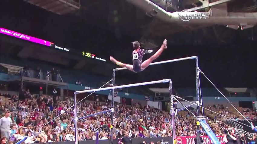
hierarchical representations for prediction. On two estab-             tributed to the advantage of hyperbolic space to represent
lished video datasets, our results show predictive hyperbolic          hierarchical structure. Following the Poincare embedding
representations are able to both recognize actions from par-           [54], [17] use a hyperbolic entailment cone to represent the
tial observations as well as forecast them in the future better        hierarchical relation in an acyclic graph. [18] further ap-
than baselines. Although our representation is trained with            plies hyperbolic geometry to feedforward neural networks
unlabeled video, visualizations also show action hierarchies           and recurrent neural networks.
automatically emerge in the hyperbolic representation. The                 Since visual data is naturally hierarchical, hyperbolic
model explicitly represents uncertainty by trading off the             space provides a strong inductive bias for images and videos
specificity versus the generality of the prediction.                   as well. [29, 11, 45] perform several image tasks, demon-
    The primary contribution of this paper is a hierar-                strating the advantage of hyperbolic embeddings over Eu-
chical representation for visual prediction. The remain-               clidean ones. [46] proposes video and action embeddings
der of this paper describes our approach and experiments               in the hyperbolic space and trains a cross-modal model to
in detail. Code and models are publicly available on                   perform hierarchical action search. We instead use hyper-
github.com/cvlab-columbia/hyperfuture.                                 bolic embeddings for prediction and we use the hierarchy to
                                                                       model uncertainty in the future. We also learn the hierarchy
2. Related Work                                                        from self-supervision, and our experiments show an action
                                                                       hierarchy emerges automatically.
    Video representation learning aims to learn strong fea-                Since dynamics are often stochastic, uncertainty repre-
tures for a number of visual video tasks. By taking advan-             sentation underpins predictive visual models. There is ex-
tage of the temporal structure in video, a line of work uses           tensive work on probabilistic models for visual prediction,
the future as incidental supervision for learning video dy-            and we only have space to briefly review. For example, [23]
namics [79, 61, 49]. Since generating pixels is challenging,           measures the covariance between outputs generated under
[52, 14, 77] instead use the natural temporal order of video           different dropout masks, which reflects how close the pre-
frames to learn self-supervised video representations. Sim-            dicted state is to the training data manifold. A high covari-
ilar to self-supervised image representations [12], temporal           ance indicates that the model is confident about its predic-
context also provides strong incidental supervision [26, 74].          tion. [2] use ensembling to estimate uncertainty, grounded
    A series of studies from Oxford has investigated how to            in the observation that a mixture of neural networks will
learn a representation in the future [21, 22] using a con-             produce dissimilar predictions if the data point is rare. An-
trastive objective. We urge readers to read these papers in            other line of work focuses on generating multiple possible
detail as they are the most related to our work. While these           future prediction, such as variational auto-encoders (VAE)
models learn predictable features, the underlying represen-            [30, 70], variational recurrent neural networks (VRNN)
tation is not adaptive to the varying levels of uncertainty in         [10, 7] and adversarial variations [40]. These models al-
natural videos. They also focus on action recognition, and             low sampling from the latent space to capture the multiple
not action prediction. By representing action hierarchies in           outcomes in the output space.
hyperbolic space, our model has robust inductive structure                 Probabilistic approaches are compatible with our frame-
for hedging uncertainty.                                               work. The main novelty of our method is that we represent
    Unlike action recognition, future action prediction [31]           the future uncertainty hierarchically in a hyperbolic space.
and early action prediction [58, 24] are tasks with an in-             The hierarchy naturally emerges during the process of learn-
trinsic uncertainty caused by the unpredictability of the fu-          ing to predict the future.
ture. Future action prediction infers future actions condi-
tioned on the current observations. Approaches for future              3. Method
prediction range from classification [53, 1], through predic-
tion of future features [67], to generation of the future at the          We present our approach for learning a hierarchical rep-
skeletal [43] or even pixel [16, 27] levels. Early action pre-         resentation of the future. We first discuss our model, then
diction aims to recognize actions before they are completely           introduce our hyperbolic representation.
executed. While standard action recognition methods can
                                                                       3.1. Predictive Model
be used for this task [57, 66], most approaches mimic a
sequential data arrival [34, 33, 75]. We evaluate our self-               Our goal is to learn a video representation that is predic-
supervised learned representations on these two tasks.                 tive of the future. Let xt ∈ RT ×W ×H×3 be a video clip
    Hyperbolic embeddings have emerged as excellent hi-                centered at time t. Instead of predicting the pixels in the
erarchical language representations in natural language pro-           future, we will predict a representation of the future. We
cessing [54, 65]. These works are pioneering. Riemmanian               denote the representation of a clip as zt = f (xt ).
optimization algorithms [6, 5] are used to optimize the mod-              The prediction task aims to forecast the unobserved rep-
els using hyperbolic geometry. Their success is largely at-            resentation zt+δ that is δ clips into the future. Given a tem-

                                                                   2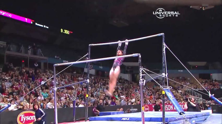
poral window of previous clips, our model estimates its pre-                                           Future                   n -D Poincaré ball
diction of zt+δ as:                                                                                   prediction

        ẑt+δ = φ(ct , δ) for         ct = g(z1 , z2 , . . . , zt )    (1)

where ct = g(·) contextually encodes features of the video
from the beginning up to and including frame t.                                                                                          Uncertain

   We will model f , g, and φ each with a neural network.
In order to learn the parameters of these models, we need
to define a distance metric between the unobserved future z                                                                             Confident
and the prediction ẑ. However, the future is often uncertain.                                 time

Instead of predicting the exact zt+δ in the future, our goal is
                                                                                  Figure 2: The future is non-deterministic. Given a specific past
to predict an abstraction that encompasses the variation of
                                                                                  (first three frames in the figure), different representations (repre-
the possible futures, and no more.                                                sented by squares in the Poincaré ball) can encode different fu-
                                                                                  tures, all of them possible. In case the model is uncertain, it will
3.2. Hierarchical Representation
                                                                                  predict an abstraction of all these possible futures, represented by
    The key contribution of this paper is to predict a hierar-                    ẑ (red square). The more confident it is, the more specific the pre-
chical representation of the future. When the future is cer-                      diction can get. Assuming the actual future is represented by z
tain, our model should predict zt+δ as specifically as pos-                       (blue square), the gray arrows represent the trajectory the predic-
sible. However, when the future is uncertain, our model                           tion will follow as more information is available. The pink circle
                                                                                  exemplifies the increase in generality when computing the mean
should “hedge the bet” and forecast a hierarchical parent of
                                                                                  of two specific representations (pink squares).
zt+δ . For example, in Fig. 1 the parent of a hand shake and
a high five is a greeting. In order to parameterize this hier-
                                                                                  that, in hyperbolic space, the mean between two leaf em-
archy, we will learn predictive models in hyperbolic space.
                                                                                  beddings is not another leaf embedding, but an embedding
    Informally, hyperbolic space can be viewed as the con-
                                                                                  that is a parent in the hierarchy. If the model cannot select
tinuous analog of a tree [54]. Unlike Euclidean space, hy-
                                                                                  between two leaf embeddings given the provided informa-
perbolic space has the unique property that circle areas and
                                                                                  tion, the expected squared distance will be minimized by
lengths grow exponentially with their radius. This den-
                                                                                  instead producing the more abstract one as the prediction.
sity allows hierarchies and trees to be compactly embedded
                                                                                      Fig. 2 visualizes this property on the Poincaré ball.
[19]. Since this space is naturally suited for hierarchies, hy-
                                                                                  Points near the center of the ball (having a smaller radius)
perbolic predictive models are able to smoothly interpolate
                                                                                  represent abstract embeddings, while points near the edge
between forecasting abstract representations (in the case of
                                                                                  (having a large radius) represent specific ones. In this ex-
low predictability) to concrete representations (in the case
                                                                                  ample, the mean of two points close to the edge of the ball—
of high predictability).
                                                                                  illustrated by the two pink squares in Fig. 2—is a node fur-
    The hyperbolic n-space, which we denote as Hn , is a
                                                                                  ther from the edge, represented with a pink circle. The line
Riemannian geometry that has constant negative curvature.2
                                                                                  connecting the two squares is the minimum distance path
While there are several models for hyperbolic space, we will
                                                                                  between them, or geodesic. The midpoint is the mean.
use the the Poincaré model, which is also the most com-
                                                                                      Unlike trees, hyperbolic space is continuous, and there
monly used in gradient-based learning. The Poincaré ball
                                                                                  is not a fixed number of hierarchy levels. Instead, there is
model is formally defined by the manifold Dn = {X ∈
                                                                                  a continuum from very specific (closer to the border of the
Rn : ||x|| < 1} and the Riemmanian metric g D : gxD = λ2x g E
                   2                E                                             Poincaré ball) to very abstract (closer to the center).
where λx := 1−kxk     2 such that g    = In is the Euclidean
metric tensor. For more details, see [41, 42].                                    3.3. Learning
    We use the Poincaré ball model to define the distance
                                                                                     To learn the parameters of the model, we want to mini-
metric between a prediction ẑ and the observation z:
                                                                                  mize the distance between the predictions ẑt and the obser-
                                      kz − ẑk2                                   vations zt . We use the contrastive learning objective func-

   dD (ẑ, z) = cosh−1 1 + 2                                (2)                   tion [21] with hyperbolic distance as the similarity measure:
                               (1 − kzk2 ) (1 − kẑk2 )
                                                                                                       "                             #
for points on the manifold Dn . Recall that the mean min-                                          X           exp −d2D (ẑ i , zi )
                                                                                            L=−         log P             2                 (3)
imizes the sum of squared residuals. The key property is                                                        j exp (−dD (ẑ i , zj ))
                                                                                                    i
    2 We assume the curvature to be −1. Hyperbolic is one of three

isotropic model spaces. The other two spaces are the Euclidean space Rn              where z is the feature representing a spatio-temporal lo-
(zero curvature), and the spherical space Sn (constant positive curvature).       cation in a video, and ẑ is the prediction of that feature. The

                                                                              3
clidean space. We therefore parameterize f , g, and φ with
                                                                        neural networks, which will be in Euclidean space. Our ap-
                                                                        proach only instantiates z and ẑ in hyperbolic space. Fig. 3
                                                                        illustrates this architecture.
    Euclidean layers                                                        In order to use this hybrid architecture, we need a pro-
    Hyperbolic layers
                                                                        jection between the two spaces. The transition from the Eu-
                        video clips                                     clidean space is based on the process mapping to Rieman-
Figure 3: Overview of architecture. Blue and red respectively in-       nian manifolds from their corresponding tangent spaces. A
dicate Euclidean and hyperbolic modules.
                                                                        Riemnnian manifold is a pair (M, g), where M is a smooth
                                                                        manifold and g is a Riemmanian metric. Broadly, smooth
contrastive objective pulls positive pairs z and ẑ together            manifolds are spaces that locally approximate Euclidean
while also pushing ẑ away from a large set of negatives,               space Rn , and on which one can differentiate [42], and this
which avoids the otherwise trivial solution. There are a va-            is precisely the connection between the two spaces. For
riety of strategies for selecting negatives [9, 64, 21]. We             x ∈ M, one can define the tangent space Tx M of M at x
create negatives from other videos in the mini batch, as well           as the first order linear approximation of M around x.
as using features that correspond to the same video but in                  The exponential map expx : Tx M → M at x is a map
different spatial or temporal locations.                                from the tangent spaces into the manifold. This projection
    The solution to the hyperbolic contrastive objective min-           is important for several operations, such as performing gra-
imizes the distance between the positive pair d2D (ẑ i , zi ).         dient updates [6]. The inverse of the exponential map is
When there is no uncertainty, the loss is minimized if ẑt =            called logarithmic map, denoted logx .
zt . However, in the face of uncertainty between two possi-
                                                                            We use an exponential map centered at 0 to project from
ble outcomes a and b, the loss is minimized by predicting
                                                                        the Euclidean space to the hyperbolic space [45]. Once the
the midpoint on the geodesic between a and b. Since hy-
                                                                        representations are in the hyperbolic space, the mathemati-
perbolic space has constant negative curvature, this solution
                                                                        cal operations and the optimization follow the rules derived
corresponds to the latent parent embedding of a and b.
                                                                        by the metric in that space. Essentially, a Riemannian met-
    Our approach treats the hierarchy as latent. Since hy-              ric defines an inner product gx that allows us to define a
perbolic space is continuous and differentiable, we are able            global distance function as the infimum of the lengths of all
to optimize Eq. 3 with stochastic gradient descent, which               curves between two points x and y [41]:
jointly learns the predictive models with the hierarchy. The
model will learn a hierarchy that is organized around the                                       d(x, y) = inf Lg (γ),                          (4)
predictability of the future.                                                                                   γ

3.4. Classification                                                     where γ : [0, 1] → M is a curve, and Lg (γ) is the length of
                                                                        the curve, defined as:
   After the representation z is trained, we are able to fit any
classifier on top of it. We use a linear classifier, and keep                         Z   1                 Z   1   q
the rest of the representation fixed (no fine-tuning). How-                Lg (γ) =           |γ̇(t)|dt =            gγ(t) (γ̇(t), γ̇(t))dt.   (5)
                                                                                      0                     0
ever, since the representation is hyperbolic, we cannot use a
standard Euclidean linear classifier. Instead, we use a hyper-              In the specific case of the Poincaré ball model, this dis-
bolic multiclass logistic regression [18] that assumes the in-          tance is the same as Eq. 2. Based on these concepts, several
put representations are in the Poincaré ball, and fits a hyper-        papers define extensions of the standard (Euclidean) neural
plane in the same space. For the Euclidean baseline we train            network layers to the hyperbolic geometry [18, 60, 8, 44,
a standard Euclidean multiclass logistic regression. In both            20]. We use the hyperbolic feed-forward layer defined in
models, we treat each node as an independent category—                  [18] to obtain the representation zD that we use in Eq. 3,
not requiring a ground truth hierarchy—when training the                from the Euclidean representation zR . Specifically, we ap-
classifier, and then compute accuracy values independently              ply this layer after the exponential map, as shown in Fig 3.
for each hierarchy level.                                               If the space is not specified, z is assumed to be zD .
                                                                            We implement f with a 3D-ResNet18, g as a one-layer
3.5. Network Architecture
                                                                        Convolutional Gated Recurrent Unit (ConvGRU) with ker-
   While we estimate our predictions and loss in hyperbolic             nel size (1, 1), and φ using a two-layer perceptron. The
space, the entire model does not need to be hyperbolic.                 dimensionality of the ResNet output is 256. When training
This flexibility enables us to take advantage of the exten-             with smaller dimensionality, we add an extra linear layer to
sive legacy of existing neural network architectures and op-            project the representations. For more implementation de-
timization algorithms that have been highly tuned for Eu-               tails, we refer the reader to the Appendix B.

                                                                    4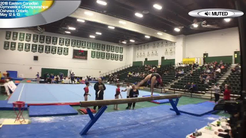
Input
videoclips
time
0.75
0.80
Poincaré 0.85
ball radius
0.90
0.95
1.00
Forecasted
category
and level
LEGEND: Uneven bars Circles Transition flight from low bar to high bar Giant circle backward Ground truth
Figure 4: We show an example of future action prediction, where the model has to determine both a hierarchy level and a class within that
level. At each time step, the model has to predict the class of the last action in the video. At the top of the figure we show the input video,
where each image represents a video clip. From the input video, the model computes a representation and a level in the hierarchy based
on the Euclidean norm of this representation. The thresholds shown in purple are the 33% percentile (dashed line) and the 66% percentile
(dotted line), ranked by the radius of predicted hyperbolic embeddings of all videos in FineGym test set. Once a level in the tree has been
determined, the model predicts the class within that level. We can see how the closer we get to the actual action to be predicted, the more
confident the model is. Also, we can see how being overly confident (by setting a low threshold and choosing a level that is too specific)
may lead the model to predict the wrong class. In this specific case, the fourth prediction (red dot) would have been more accurate had the
model predicted a class in the parent level (i.e. had it predicted the blue dot). Note that the y-axis is inverted in the graph. Also, the nodes
represented in the tree are not all the classes in the FineGym dataset, and each node has more children not shown.
time Forecasted time
category and level Forecasted
category and level
Floor exercise Leap, jump, hop Switch leap (leap forward with leg to cross split) Human interaction Handshake Hug Forecast
Balance Beam Flight salto Round-off Car interaction Driving Open door car
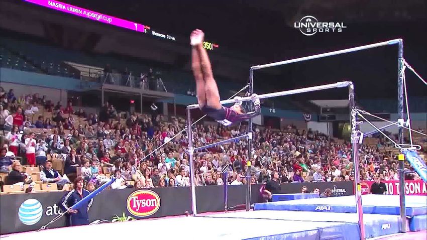
Figure 5: We show four more examples where the model correctly predicts the class at different hierarchical levels. The FineGym examples
(left) are evaluated on future action prediction, and the Hollywood2 ones (right) on early action prediction, where we show the model half
of the clips in the video. The shown trees are just partial representations of the complete hierarchies. Click here for video visualizations.
4. Experiments dataset. On the target domain, we fine-tune on the same ob-
jective before fitting a supervised linear classifier on ẑ using
The basic objective of our experiments is to analyze how a small number of labeled examples.
hyperbolic representations encode varying levels of uncer-
tainty in the future. We quantitatively evaluate on two dif- We evaluate on two different video datasets, which we
ferent tasks and two different datasets. We also show several selected for their realistic temporal structure:
visualizations and diagnostic analysis. Sports Videos: In this setting, we learn the self-
supervised representation on Kinetics-600 [28] and fine-
4.1. Datasets and Common Setup
tune and evaluate on FineGym [59]. Kinetics has 600 hu-
We use a common evaluation setup throughout our ex- man action classes and 500, 000 of videos which contain
periments. We first learn a self-supervised representation rich and diverse human actions. We discard its labels. Fin-
from a large collection of unlabeled videos by optimizing eGym is a dataset of gymnastic videos where clips are an-
Eq. 3. After learning the representation, we transfer these notated with three-level hierarchical action labels, ranging
representations to the target domain using a smaller, labeled from specific exercise names in the lowest level to generic
5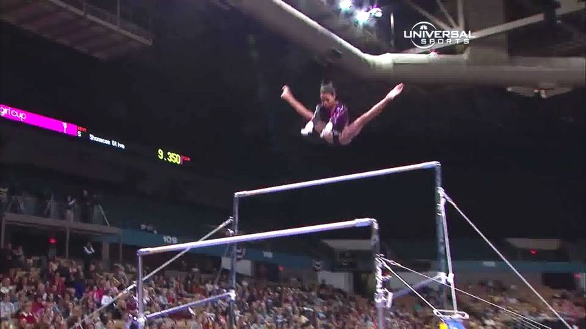
Representation    Dim. Accuracy (%)

                                             0.7
                                                                                      Hyperbolic (ours) 256     82.54
                                                                                      Euclidean [21]    256     68.16
                                                                                      Hyperbolic (ours) 64      73.35
                                                                                      Euclidean [21]     64     66.04
                                                                                      Most common               35.40

                                                0.8
                                                                                      Chance                    25.00
                                                                           Table 1: Early action prediction on FineGym. We do not report hi-
                                                                           erarchical accuracy because FineGym only annotates the hierarchy
                                                                           at the clip level, not video level. See Section 4.4 for discussion.

                                                   0.9
                                                                                                                    Top-down Bottom-up
                                                                            Representation      Dim. Accuracy
Figure 6: Trajectories showing the evolution with time of the pre-                                                  hier. acc. hier. acc.
dictions in Kinetics, where the task consists in predicting features        Hyperbolic (ours)    256      23.10       33.99      28.55
of the last video clip. We show the two dimensions with larger              Euclidean [21]       256      21.77       33.00      27.38
values across all the predictions. Each line represents a prediction        Hyperbolic (ours)     64      22.25       31.47      26.86
for a specific video.                                                       Euclidean [21]        64      15.47       24.09      19.78
                                                                            Most common                   17.08       25.19      21.13
                                                                            Chance                        8.33        16.11      12.22
gymnastic routines (e.g. balance-beam) in the highest one.
                                                                           Table 2: Early action prediction on Hollywood2. See Section 4.4.
The highest level of the hierarchy is consistent for all the
clips in a video, so we use it as a label for the whole video.
   Movies: In our second setting, we learn the self-                       cases, higher is better.
supervised representation on MovieNet [25], then fine-tune
and evaluate the Hollywood2 dataset [48]. MovieNet con-
                                                                           4.3. Baselines
tains 1, 100 movies and 758, 000 key frames. In order to                      The main goal of the paper is to compare hyperbolic rep-
obtain a hierarchy of actions from Hollywood2 at the video                 resentations to Euclidean ones [21]. We therefore present
level, we grouped action classes into more general ones to                 our experiments on comparisons between these two spaces,
form a 2-level hierarchy. The hierarchy is shown in the                    keeping the rest of the method the same. It is worth noting
Appendix A. Since Hollywood2 does not have fine-grained                    that [21] has state-of-the-art results for several video tasks
clip-level action labels like FineGym, we do not evaluate                  among self-supervised video approaches. Additionally, we
future action prediction on this dataset.                                  report chance accuracy, resulting from randomly selecting a
                                                                           class, and the most common strategy, which always selects
4.2. Evaluation metrics                                                    the most common class in the training set.
    In our quantitative evaluation, our goal is twofold. First,               Trees are compact in hyperbolic space. We show results
we want to evaluate that the obtained representations are                  for feature spaces with 256 dimensions, as in [21], as well
better at modeling scenarios with high uncertainty. Second,                as 64 dimensions.
we want to analyze the hierarchical structure of the learned
space. We use three different metrics:                                     4.4. Early Action Recognition
    Accuracy: Standard classification accuracy. Compares                       We first evaluate on the early action recognition task,
only classes at the lowest (most specific) hierarchical level.             which aims to classify actions that have started, but not
    Bottom-up hierarchical accuracy: A prediction is con-                  finished yet. In other words, the observed video is only
sidered partially correct if it predicts the wrong node at the             partially completed, producing uncertainty. We use video-
leaf level but the correct nodes at upper levels. We weigh                 level action labels to train the classification layer on ẑN (ct ),
each level with a reward that decays by 50% as we go up in                 for all time steps t. Tab. 1 and Tab. 2 show that, with ev-
the hierarchy tree.                                                        erything else fixed, hyperbolic models learn significantly
    Top-down hierarchical accuracy: In the hierarchical                    better representations than the Euclidean counterparts (up
metrics literature it is sometimes argued that predicting the              to 14% gain). The hyperbolic representation enjoys sub-
root node correctly is more important than predicting the                  stantial compression efficiency, indicated by the 64 dimen-
exact leaf node [78]. Therefore we also report the accuracy                sional hyperbolic embedding outperforming the larger 256
value that gives the root node a weight of 1, and decreases                dimensional Euclidean embedding (up to 5%). As indicated
it the closer we get to the leaf node, also by a factor of 1/2.            by both hierarchical accuracy metrics, when there is uncer-
    For clarity, in both hierarchical evaluations we normal-               tainty, the hyperbolic representation will predict a more ap-
ize the accuracy to be always within the [0, 1] range. In all              propriate parent than Euclidean representations.

                                                                       6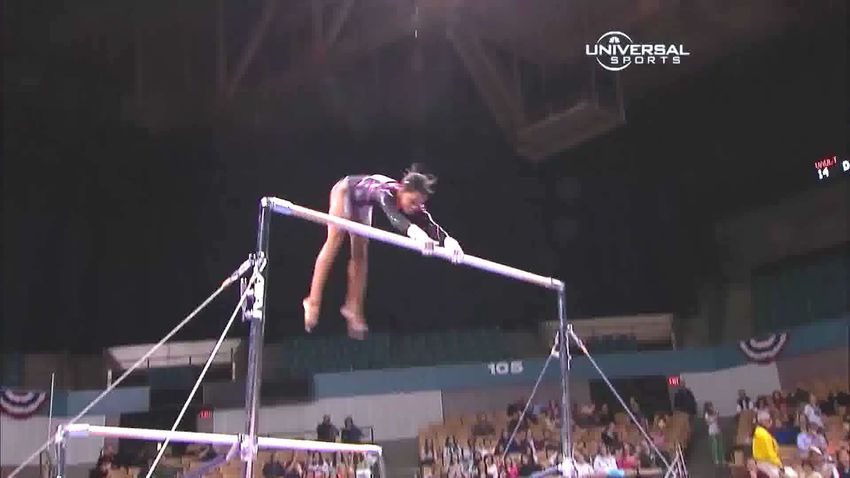
Top-down Bottom-up
Representation Dim. Accuracy
time hier. acc. hier. acc.
200 47 16 10 1
Hyperbolic (ours) 256 13.37 66.64 33.04
Euclidean [21] 256 10.08 52.00 24.75
...
... Hyperbolic (ours) 64 10.29 56.67 27.49
Table 1 Euclidean [21] 64 9.26 52.41 26.22
1 2 3
Most
4
common 5
3.646 27.90 12.75
Movies:
Chance 0.00 16.24 5.67
0.2248 0.2271 0.2375 0.2375 0.226 0.2399
Hyperbolic
... Table 3: Future action prediction on FineGym. See Section 4.5.
Movies: Euclidean 0.2063 0.2121 0.2202 0.2225 0.2178 0.2271
1.00
Figure 7: The area of the circle is proportional to the number of
0.98
videos retrieved within a certain threshold distance. The more spe-
Poincaré ball radius
0.96
cific the prediction gets, the further most of the clips are (only a
few ones get closer). The threshold is computed as the mean of all 0.94
the distances from predictions to clip features. Note that the last 0.92
circle does not necessarily have to contain exactly one video clip. 0.90
The total number of clips for this retrieval experiment was 300. 0.88 Kinetics
MovieNet
0.86 Hollywood2
Movies: Hyperbolic Sports: Hyperbolic 0.84 FineGym
Movies: Euclidean Sports: Euclidean
0.25 0.90 t-6 t-5 t-4 t-3 t-2 t-1 t
0.24 0.83
Accuracy
Accuracy
Prediction time step
0.23 0.75
0.21 0.68 Figure 9: We visualize how the radius of predicted features evolve
0.20 0.60
1 2 3 4 5 6 5 4 3 2 1 0 as more data is observed. The larger the radius, the more confident
Time Elapsed (Early) Time into Future (Forecasting) and more specific the prediction becomes.
Figure 8: Classification accuracy for early action prediction (left)
and future action prediction (right). Performance increases as the thresholds are set, we obtain both the predicted hierarchy
model receives more observations or predicts closer to the target. level as well as the predicted class within that level.
Table
For all horizons, the hyperbolic representation is more 2
accurate.
Table 3 compares our predictive models versus the base-
5 4 3 2 1 0
line in Euclidean space. We report values for t = N − 1.
4.5. Future Action Prediction
Sports: Hyperbolic 0.7847 0.8194 0.8299 0.842 0.8446 0.8456
For all three metrics, predicting a hierarchical representa-
Sports: Euclidean 0.6319 0.6727 0.6884 0.6936 0.6979 0.7049
We next evaluate the representation on future action pre- tion substantially outperforms baselines by up to 14 points.
diction, which aims to predict actions before they start given The gains in both top-down and bottom-up hierarchical ac-
the past context. There is uncertainty because the next ac- curacy show that our model selects a better level of abstrac-
tions are not deterministic. tion than the baselines in the presence of uncertainty. We
A key advantage of hyperbolic representations is that the visualize the hyperbolic representation and the resulting hi-
model will automatically decide to select the level of ab- erarchical predictions in Fig. 4. We show more examples of
straction based on its estimate of the uncertainty. If the pre- forecasted levels and classes in Fig 5.
diction is closer to the center of the Poincaré ball, the model The hyperbolic model also obtains better performance
lacks confidence and it predicts a parental node close to the than the Euclidean model at the standard classification ac-
root in the hierarchy. If the prediction is closer to the bor- curacy, which only evaluates the leaf node prediction. Since
der of the Poincaré ball, the model is more confident and classification accuracy does not account for the hierar-
consequently predicts a more specific outcome. chy, this gain suggests hyperbolic representations help even
We fine-tune our model to learn to predict the class of when the future is certain. We hypothesize this is because
the last clip of a video at each time step, for each of the the model is explicitly representing uncertainty, which sta-
three hierarchy levels in the FineGym dataset. We use clip- bilizes the training compared to the Euclidean baseline.
level labels to train the classification layer on the model’s Since our model represents its prediction of the uncer-
prediction ẑN (ct ). We select a threshold between hierarchy tainty, we are able to visualize which videos are predictable.
levels by giving each level the same probability of being se- Fig. 10 visualizes several examples.
lected: the predictions that have a radius in the smaller than
the 33% percentile will select the more general level, the 4.6. Analysis of the Representation
ones above the 66% percentile will select the more specific We next analyze the emergent properties of the learned
level, and the rest will select the middle level.3 Once the representations, and how they change as more information
1
3 These
thresholds can be modified according to the risk tolerance of is given to the model. We conduct our analysis on the self-
the application. supervised representation, before supervised fine-tuning.
7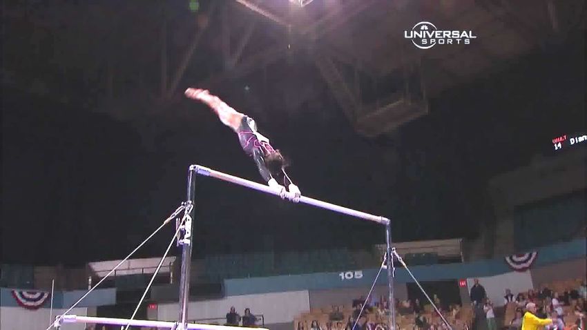
Predictable future                                                 Unpredictable future
Hollywood2
MovieNet
Kinetics

Figure 10: We show examples with high predictability (left), and low predictability (right). The first two frames represent the content the
model sees, and the frame in green represents the action the model has to predict. The high predictability examples are selected from above
the 99 percentile and the low predictability examples are selected from below the 1 percentile, measured by the radius of the prediction.
In both Hollywood2 and MovieNet, the model is more certain about static actions, where the future is close to the past. Specifically in
MovieNet we found that most of the highly predictable clips involved close-up conversations of people. The unpredictable ones correspond
mostly to action scenes where the future possibilities are very diverse. In the Kinetics dataset, we also noticed that most of the predictable
futures corresponded to videos with static people, and the unpredictable ones were associated generally to sports.

    Fig. 6 visualizes the trajectory that representations fol-                 video clips belonging to the same event and gymnastics in-
low as frames are continuously observed. We visualize the                      strument in FineGym, we compute features for each one of
representation from Kinetics. In order to plot a 2D graph,                     the clips in these videos, that we use as targets to retrieve.
we select the two dimensions with the highest mean value,                      For each video, we then predict the last representation at
and plot their trajectories with the time.4 The red dots show                  each time step (i.e., for every clip in the video), and use
the actual features that have to be predicted. As the ob-                      these as queries. We show the results for one such videos
servations get closer to its prediction target, predictions get                in Fig. 7. The retrieved number corresponds to the num-
closer to the edge of the Poincaré ball, indicating they are                  ber of clips that are in a distance within a threshold, that
becoming more specific in the hierarchy and increasingly                       we compute as the mean of all the distances from predic-
confident about the prediction.                                                tions to features. As the time horizon to the target action
    The distance to the center of the Poincaré ball gives us in-              shrinks, the more specific the representation becomes, and
tuition about the underlying geometry, and Fig. 9 quantifies                   thus fewer options are recalled. Fig. 8 quantifies perfor-
this behavior. We show the average radius of the predictions                   mance versus time horizon, showing the hyperbolic repre-
at each time step, together with the standard deviation. As                    sentation is more accurate than the Euclidean representation
more frames become available, the prediction gets consis-                      for all time periods.
tently more confident for all datasets.
                                                                               5. Conclusion
    Abstract predictions will encompass a large number of
specific features that can be predicted, while specific pre-                      While there is uncertainty in the future, parts of it are
dictions will restrict the options to just a few. We visualize                 predictable. We have introduced a hyperbolic model for
these predictions using nearest neighbors. Given a series of                   video prediction that represents uncertainty hierarchically.
                                                                               After learning from unlabeled video, experiments and visu-
    4 Projecting using TSNE [47] or uMAP [50] does not respect the local       alizations show that a hierarchy automatically emerges in
structure well enough to visualize the radius of the prediction.               the representation, encoding the predictability of the future.

                                                                           8
Acknowledgments: We thank Will Price, Mia Chiquier, Dave              [12] Carl Doersch, Abhinav Gupta, and Alexei A Efros. Unsuper-
Epstein, Sarah Gu, and Ishaan Chandratreya for helpful feed-                   vised visual representation learning by context prediction. In
back. This research is based on work partially supported by NSF                Proceedings of the IEEE international conference on com-
NRI Award #1925157, the DARPA MCS program under Federal                        puter vision, pages 1422–1430, 2015. 2
Agreement No. N660011924032, the DARPA KAIROS program                     [13] Debidatta Dwibedi, Yusuf Aytar, Jonathan Tompson, Pierre
under PTE Federal Award No. FA8750-19-2-1004, and an Ama-                      Sermanet, and Andrew Zisserman.             Temporal cycle-
                                                                               consistency learning. In Proceedings of the IEEE Conference
zon Research Gift. We thank NVidia for GPU donations. The
                                                                               on Computer Vision and Pattern Recognition, pages 1801–
views and conclusions contained herein are those of the authors
                                                                               1810, 2019. 1
and should not be interpreted as necessarily representing the offi-
                                                                          [14] Basura Fernando, Hakan Bilen, Efstratios Gavves, and
cial policies, either expressed or implied, of the U.S. Government.            Stephen Gould. Self-supervised video representation learn-
                                                                               ing with odd-one-out networks. In Proceedings of the
References                                                                     IEEE conference on computer vision and pattern recogni-
 [1] Yazan Abu Farha, Alexander Richard, and Juergen Gall.                     tion, pages 3636–3645, 2017. 1, 2
     When will you do what?-anticipating temporal occurrences             [15] Katerina Fragkiadaki, Pulkit Agrawal, Sergey Levine, and
     of activities. In Proceedings of the IEEE conference on                   Jitendra Malik. Learning visual predictive models of physics
     computer vision and pattern recognition, pages 5343–5352,                 for playing billiards. arXiv preprint arXiv:1511.07404,
     2018. 1, 2                                                                2015. 1
 [2] Charles Blundell Balaji Lakshminarayanan, Alexander                  [16] Harshala Gammulle, Simon Denman, Sridha Sridharan, and
     Pritzel. Simple and Scalable Predictive Uncertainty Estima-               Clinton Fookes. Predicting the future: A jointly learnt model
     tion using Deep Ensembles. NIPS, 2017. 2                                  for action anticipation. In Proceedings of the IEEE Inter-
 [3] Christopher Baldassano, Janice Chen, Asieh Zadbood,                       national Conference on Computer Vision, pages 5562–5571,
     Jonathan W Pillow, Uri Hasson, and Kenneth A Norman.                      2019. 2
     Discovering event structure in continuous narrative percep-          [17] Octavian-Eugen Ganea, Gary Bécigneul, and Thomas Hof-
     tion and memory. Neuron, 95(3):709–721, 2017. 1                           mann. Hyperbolic entailment cones for learning hierarchi-
 [4] Roger G Barker and Herbert F Wright. Midwest and its chil-                cal embeddings. 35th International Conference on Machine
     dren: The psychological ecology of an american town. 1955.                Learning, ICML 2018, 4:2661–2673, 2018. 2
     1                                                                    [18] Octavian-Eugen Ganea, Gary Bécigneul, and Thomas Hof-
 [5] Gary Becigneul and Octavian-Eugen Ganea. Riemannian                       mann. Hyperbolic neural networks. Advances in Neural In-
     adaptive optimization methods. In International Conference                formation Processing Systems, 2018-December:5345–5355,
     on Learning Representations, 2019. 2, 12                                  2018. 2, 4
 [6] Silvere Bonnabel. Stochastic gradient descent on rieman-             [19] Michael Gromov. Hyperbolic groups. In Essays in group
     nian manifolds. IEEE Transactions on Automatic Control,                   theory, 1987. 1, 3
     58(9):2217–2229, 2013. 2, 4                                          [20] Caglar Gulcehre, Misha Denil, Mateusz Malinowski, Ali
 [7] Lluis Castrejon, Nicolas Ballas, and Aaron Courville. Im-                 Razavi, Razvan Pascanu, Karl Moritz Hermann, Peter
     proved conditional vrnns for video prediction. In Proceed-                Battaglia, Victor Bapst, David Raposo, Adam Santoro, and
     ings of the IEEE International Conference on Computer Vi-                 Nando de Freitas. Hyperbolic attention networks. 7th In-
     sion, pages 7608–7617, 2019. 2                                            ternational Conference on Learning Representations, ICLR
 [8] Ines Chami, Zhitao Ying, Christopher Ré, and Jure                        2019, i:1–15, 2019. 4
     Leskovec. Hyperbolic graph convolutional neural networks.            [21] Tengda Han, Weidi Xie, and Andrew Zisserman. Video rep-
     In Advances in neural information processing systems, pages               resentation learning by dense predictive coding. In Proceed-
     4868–4879, 2019. 4                                                        ings of the IEEE International Conference on Computer Vi-
 [9] Ting Chen, Simon Kornblith, Mohammad Norouzi, and Ge-                     sion Workshops, pages 0–0, 2019. 1, 2, 3, 4, 6, 7, 12
     offrey Hinton. A simple framework for contrastive learning           [22] Tengda Han, Weidi Xie, and Andrew Zisserman. Memory-
     of visual representations. arXiv preprint arXiv:2002.05709,               augmented dense predictive coding for video representation
     2020. 4                                                                   learning. arXiv preprint arXiv:2008.01065, 2020. 2
[10] Junyoung Chung, Kyle Kastner, Laurent Dinh, Kratarth                 [23] Mikael Henaff, Yann LeCun, and Alfredo Canziani. Model-
     Goel, Aaron Courville, and Yoshua Bengio. A recurrent                     predictive policy learning with uncertainty regularization for
     latent variable model for sequential data. Advances in                    driving in dense traffic. 7th International Conference on
     Neural Information Processing Systems, 2015-Janua:2980–                   Learning Representations, ICLR 2019, pages 1–20, 2019. 2
     2988, 2015. 2                                                        [24] Minh Hoai and Fernando De la Torre. Max-margin early
[11] Ankit Dhall, Anastasia Makarova, Octavian Ganea, Dario                    event detectors. International Journal of Computer Vision,
     Pavllo, Michael Greeff, and Andreas Krause. Hierarchi-                    107(2):191–202, 2014. 2
     cal image classification using entailment cone embeddings.           [25] Qingqiu Huang, Yu Xiong, Anyi Rao, Jiaze Wang, and
     IEEE Computer Society Conference on Computer Vision                       Dahua Lin. Movienet: A holistic dataset for movie un-
     and Pattern Recognition Workshops, 2020-June:3649–3658,                   derstanding. In European Conference on Computer Vision
     2020. 2                                                                   (ECCV), 2020. 6

                                                                      9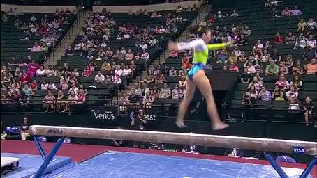
[26] Phillip Isola, Daniel Zoran, Dilip Krishnan, and Edward H                  Translation via Disentangled Representations. Lecture Notes
     Adelson. Learning visual groups from co-occurrences in                     in Computer Science (including subseries Lecture Notes in
     space and time. Workshop track - ICLR 2016, 2015. 2                        Artificial Intelligence and Lecture Notes in Bioinformatics),
[27] Dinesh Jayaraman, Frederik Ebert, Alexei A Efros, and                      11205 LNCS:36–52, 2018. 2
     Sergey Levine. Time-agnostic prediction: Predicting pre-            [41]   John M Lee. Riemannian manifolds: an introduction to cur-
     dictable video frames. arXiv preprint arXiv:1808.07784,                    vature, volume 176. Springer Science & Business Media,
     2018. 2                                                                    2006. 3, 4
[28] Will Kay, Joao Carreira, Karen Simonyan, Brian Zhang,               [42]   John M Lee. Smooth manifolds. In Introduction to Smooth
     Chloe Hillier, Sudheendra Vijayanarasimhan, Fabio Viola,                   Manifolds, pages 1–31. Springer, 2013. 3, 4
     Tim Green, Trevor Back, Paul Natsev, et al. The kinetics hu-        [43]   Chen Li, Zhen Zhang, Wee Sun Lee, and Gim Hee Lee. Con-
     man action video dataset. arXiv preprint arXiv:1705.06950,                 volutional sequence to sequence model for human dynamics.
     2017. 5                                                                    In Proceedings of the IEEE Conference on Computer Vision
[29] Valentin Khrulkov, Leyla Mirvakhabova, Evgeniya Usti-                      and Pattern Recognition, pages 5226–5234, 2018. 2
     nova, Ivan Oseledets, and Victor Lempitsky. Hyperbolic              [44]   Qi Liu, Maximilian Nickel, and Douwe Kiela. Hyperbolic
     image embeddings. In Proceedings of the IEEE/CVF Con-                      graph neural networks. In Advances in Neural Information
     ference on Computer Vision and Pattern Recognition, pages                  Processing Systems, pages 8230–8241, 2019. 4
     6418–6428, 2020. 2                                                  [45]   Shaoteng Liu, Jingjing Chen, Liangming Pan, Chong-Wah
[30] Diederik P. Kingma and Max Welling. Auto-encoding varia-                   Ngo, Tat-Seng Chua, and Yu-Gang Jiang. Hyperbolic Visual
     tional bayes. 2nd International Conference on Learning Rep-                Embedding Learning for Zero-Shot Recognition. In Com-
     resentations, ICLR 2014 - Conference Track Proceedings,                    puter Vision and Pattern Recognition, pages 9273—-9281,
     pages 1–14, 2014. 2                                                        2020. 2, 4
[31] Kris M Kitani, Brian D Ziebart, James Andrew Bagnell, and           [46]   Teng Long, Pascal Mettes, Heng Tao Shen, and Cees Snoek.
     Martial Hebert. Activity forecasting. In European Confer-                  Searching for Actions on the Hyperbole. Cvpr, pages 1138–
     ence on Computer Vision, pages 201–214. Springer, 2012. 1,                 1147, 2020. 2
     2                                                                   [47]   Laurens van der Maaten and Geoffrey Hinton. Visualiz-
                                                                                ing data using t-sne. Journal of machine learning research,
[32] Max Kochurov, Rasul Karimov, and Serge Kozlukov.
                                                                                9(Nov):2579–2605, 2008. 8
     Geoopt: Riemannian optimization in pytorch, 2020. 12
                                                                         [48]   Marcin Marszałek, Ivan Laptev, and Cordelia Schmid. Ac-
[33] Yu Kong, Dmitry Kit, and Yun Fu. A discriminative model
                                                                                tions in context. In IEEE Conference on Computer Vision &
     with multiple temporal scales for action prediction. In
                                                                                Pattern Recognition, 2009. 6
     European conference on computer vision, pages 596–611.
                                                                         [49]   Michael Mathieu, Camille Couprie, and Yann LeCun. Deep
     Springer, 2014. 2
                                                                                multi-scale video prediction beyond mean square error.
[34] Yu Kong, Zhiqiang Tao, and Yun Fu. Deep sequential con-
                                                                                arXiv preprint arXiv:1511.05440, 2015. 1, 2
     text networks for action prediction. In Proceedings of the
                                                                         [50]   Leland McInnes, John Healy, and James Melville. Umap:
     IEEE Conference on Computer Vision and Pattern Recogni-
                                                                                Uniform manifold approximation and projection for dimen-
     tion, pages 1473–1481, 2017. 2
                                                                                sion reduction. arXiv preprint arXiv:1802.03426, 2018. 8
[35] Hema S Koppula and Ashutosh Saxena. Anticipating hu-                [51]   Antoine Miech, Jean-Baptiste Alayrac, Lucas Smaira, Ivan
     man activities using object affordances for reactive robotic               Laptev, Josef Sivic, and Andrew Zisserman. End-to-End
     response. IEEE transactions on pattern analysis and ma-                    Learning of Visual Representations from Uncurated Instruc-
     chine intelligence, 38(1):14–29, 2015. 1                                   tional Videos. In CVPR, 2020. 1
[36] Zoe Kourtzi and Nancy Kanwisher. Activation in human                [52]   Ishan Misra, C Lawrence Zitnick, and Martial Hebert. Shuf-
     mt/mst by static images with implied motion. Journal of                    fle and learn: unsupervised learning using temporal order
     cognitive neuroscience, 12(1):48–55, 2000. 1                               verification. In European Conference on Computer Vision,
[37] Manoj Kumar, Mohammad Babaeizadeh, Dumitru Erhan,                          pages 527–544. Springer, 2016. 1, 2
     Chelsea Finn, Sergey Levine, Laurent Dinh, and Durk                 [53]   Yan Bin Ng and Basura Fernando. Forecasting future se-
     Kingma. Videoflow: A conditional flow-based model for                      quence of actions to complete an activity. arXiv preprint
     stochastic video generation. In International Conference on                arXiv:1912.04608, 2019. 2
     Learning Representations, 2019. 1                                   [54]   Maximillian Nickel and Douwe Kiela.            Poincaré em-
[38] Yong-Hoon Kwon and Min-Gyu Park. Predicting future                         beddings for learning hierarchical representations. Ad-
     frames using retrospective cycle gan. In Proceedings of the                vances in Neural Information Processing Systems, 2017-
     IEEE Conference on Computer Vision and Pattern Recogni-                    December(Nips):6339–6348, 2017. 1, 2, 3
     tion, pages 1811–1820, 2019. 1                                      [55]   Adam Paszke, Sam Gross, Francisco Massa, Adam Lerer,
[39] Hsin-Ying Lee, Jia-Bin Huang, Maneesh Singh, and Ming-                     James Bradbury, Gregory Chanan, Trevor Killeen, Zeming
     Hsuan Yang. Unsupervised representation learning by sort-                  Lin, Natalia Gimelshein, Luca Antiga, Alban Desmaison,
     ing sequences. In Proceedings of the IEEE International                    Andreas Kopf, Edward Yang, Zachary DeVito, Martin Rai-
     Conference on Computer Vision, pages 667–676, 2017. 1                      son, Alykhan Tejani, Sasank Chilamkurthy, Benoit Steiner,
[40] Hsin Ying Lee, Hung Yu Tseng, Jia Bin Huang, Maneesh                       Lu Fang, Junjie Bai, and Soumith Chintala. Pytorch: An im-
     Singh, and Ming Hsuan Yang. Diverse Image-to-Image                         perative style, high-performance deep learning library. In H.

                                                                    10
Wallach, H. Larochelle, A. Beygelzimer, F. d'Alché-Buc, E. using variational autoencoders. In European Conference on
Fox, and R. Garnett, editors, Advances in Neural Informa- Computer Vision, pages 835–851. Springer, 2016. 1, 2
tion Processing Systems 32, pages 8024–8035. Curran Asso- [71] Jacob Walker, Abhinav Gupta, and Martial Hebert. Patch
ciates, Inc., 2019. 12 to the future: Unsupervised visual prediction. In Proceed-
[56] MarcAurelio Ranzato, Arthur Szlam, Joan Bruna, Michael ings of the IEEE conference on Computer Vision and Pattern
Mathieu, Ronan Collobert, and Sumit Chopra. Video (lan- Recognition, pages 3302–3309, 2014. 1
guage) modeling: a baseline for generative models of natural [72] Jacob Walker, Kenneth Marino, Abhinav Gupta, and Martial
videos. arXiv preprint arXiv:1412.6604, 2014. 1 Hebert. The pose knows: Video forecasting by generating
[57] Michalis Raptis and Leonid Sigal. Poselet key-framing: A pose futures. In Proceedings of the IEEE international con-
model for human activity recognition. In Proceedings of the ference on computer vision, pages 3332–3341, 2017. 1
IEEE Conference on Computer Vision and Pattern Recogni- [73] Jiangliu Wang, Jianbo Jiao, Linchao Bao, Shengfeng He,
tion, pages 2650–2657, 2013. 2 Yunhui Liu, and Wei Liu. Self-supervised spatio-temporal
[58] Michael S Ryoo. Human activity prediction: Early recog- representation learning for videos by predicting motion and
nition of ongoing activities from streaming videos. In 2011 appearance statistics. In Proceedings of the IEEE Conference
International Conference on Computer Vision, pages 1036– on Computer Vision and Pattern Recognition, pages 4006–
1043. IEEE, 2011. 2 4015, 2019. 1
[59] Dian Shao, Yue Zhao, Bo Dai, and Dahua Lin. Finegym: A [74] Xiaolong Wang and Abhinav Gupta. Unsupervised learn-
hierarchical video dataset for fine-grained action understand- ing of visual representations using videos. In Proceedings of
ing. In IEEE Conference on Computer Vision and Pattern the IEEE international conference on computer vision, pages
Recognition (CVPR), 2020. 5 2794–2802, 2015. 1, 2
[60] Ryohei Shimizu, Yusuke Mukuta, and Tatsuya Harada. Hy- [75] Xionghui Wang, Jian-Fang Hu, Jian-Huang Lai, Jianguo
perbolic neural networks++, 2020. 4 Zhang, and Wei-Shi Zheng. Progressive teacher-student
[61] Nitish Srivastava, Elman Mansimov, and Ruslan Salakhudi- learning for early action prediction. In Proceedings of the
nov. Unsupervised learning of video representations using IEEE Conference on Computer Vision and Pattern Recogni-
lstms. In International conference on machine learning, tion, pages 3556–3565, 2019. 2
pages 843–852, 2015. 2 [76] Xiaolong Wang, Allan Jabri, and Alexei A Efros. Learning
[62] Kimberly L Stachenfeld, Matthew M Botvinick, and correspondence from the cycle-consistency of time. In Pro-
Samuel J Gershman. The hippocampus as a predictive map. ceedings of the IEEE Conference on Computer Vision and
Nature neuroscience, 20(11):1643, 2017. 1 Pattern Recognition, pages 2566–2576, 2019. 1
[63] Chen Sun, Fabien Baradel, Kevin Murphy, and Cordelia [77] Donglai Wei, Joseph J Lim, Andrew Zisserman, and
Schmid. Contrastive bidirectional transformer for temporal William T Freeman. Learning and using the arrow of time.
representation learning. In arXiv, June 2019. 1 In Proceedings of the IEEE Conference on Computer Vision
[64] Yonglong Tian, Dilip Krishnan, and Phillip Isola. Con- and Pattern Recognition, pages 8052–8060, 2018. 2
trastive multiview coding. arXiv preprint arXiv:1906.05849, [78] Cinna Wu, Mark Tygert, and Yann LeCun. A hierarchical
2019. 4 loss and its problems when classifying non-hierarchically.
[65] Alexandru Tifrea, Gary Bécigneul, and Octavian-Eugen Plos one, 14(12):e0226222, 2019. 6
Ganea. Poincaré Glove: Hyperbolic word embeddings. [79] SHI Xingjian, Zhourong Chen, Hao Wang, Dit-Yan Yeung,
7th International Conference on Learning Representations, Wai-Kin Wong, and Wang-chun Woo. Convolutional lstm
ICLR 2019, 2019. 2 network: A machine learning approach for precipitation
[66] Arash Vahdat, Bo Gao, Mani Ranjbar, and Greg Mori. A nowcasting. In Advances in neural information processing
discriminative key pose sequence model for recognizing hu- systems, pages 802–810, 2015. 2
man interactions. In 2011 IEEE International Conference [80] Dejing Xu, Jun Xiao, Zhou Zhao, Jian Shao, Di Xie, and
on Computer Vision Workshops (ICCV Workshops), pages Yueting Zhuang. Self-supervised spatiotemporal learning via
1729–1736. IEEE, 2011. 2 video clip order prediction. In Proceedings of the IEEE Con-
[67] Carl Vondrick, Hamed Pirsiavash, and Antonio Torralba. An- ference on Computer Vision and Pattern Recognition, pages
ticipating visual representations from unlabeled video. In 10334–10343, 2019. 1
Proceedings of the IEEE Conference on Computer Vision [81] Jenny Yuen and Antonio Torralba. A data-driven approach
and Pattern Recognition, pages 98–106, 2016. 1, 2 for event prediction. In European Conference on Computer
[68] Carl Vondrick, Hamed Pirsiavash, and Antonio Torralba. Vision, pages 707–720. Springer, 2010. 1
Generating videos with scene dynamics. In Advances in neu-
ral information processing systems, pages 613–621, 2016. 1
[69] Carl Vondrick, Abhinav Shrivastava, Alireza Fathi, Sergio
Guadarrama, and Kevin Murphy. Tracking emerges by col-
orizing videos. In Proceedings of the European conference
on computer vision (ECCV), pages 391–408, 2018. 1
[70] Jacob Walker, Carl Doersch, Abhinav Gupta, and Martial
Hebert. An uncertain future: Forecasting from static images
11Appendix are short, in which case we use the maximum size allowed
by the dataset. Following [21] we use H = W = 128.
A. Hollywood2 Hierarchy We optimize our objective using Riemannian Adam [5]
and the Geoopt library in Pytorch [32, 55]. We train our
Hollywood2 (Root) models with a batch size of 128 for 100 epochs. We tried
three learning rates (10−2 , 10−3 , 10−4 ). We select the
Car Interaction model with better accuracy on a held-out validation set.
We select positives and negatives using the same strategy
Drive Car
as [21], augmenting it with δ values larger than 1.
Get Out Car
Handle Tools
Answer Phone
Eat
Interact with Human
Hug Person
Kiss
Hand Shake
Fast Human Action
Fight Person
Run
Body Motion
Sit Down
Sit Up
Stand Up
B. Implementation Details
Code and models are publicly available on
github.com/cvlab-columbia/hyperfuture.
We implement f with a 3D-ResNet18, and g as a one-
layer Convolutional Gated Recurrent Unit (ConvGRU) with
kernel size (1, 1). We implement φ using a two-layer per-
ceptron. The dimensionality at the output of the ResNet
is 256. When training with representations with smaller
dimensionality, we add an extra linear layer to project the
representations.
Before inputting representations to the classification
layer, we mean pool them spatially, in the Euclidean space.
In order to select video clips, we subsample N non-
overlapping blocks from the original video, consisting of
T frames each. In cases where divisions into clips are given
by the dataset, we use those as inputs. By default, we use
T = 5 except for datasets where clips are shorter than 5
frames, in which case we use the size of the given clip.
Similarly, we set N = 8 except in datasets where videos
12You can also read