Activation of optimally and unfavourably oriented faults in a uniform local stress field during the 2011 Prague, Oklahoma, sequence
←
→
Page content transcription
If your browser does not render page correctly, please read the page content below
Geophys. J. Int. (2020) 222, 153–168                                                                                         doi: 10.1093/gji/ggaa153
Advance Access publication 2020 March 29
GJI Seismology

Activation of optimally and unfavourably oriented faults in a uniform
local stress field during the 2011 Prague, Oklahoma, sequence

Elizabeth S. Cochran ,1 Robert J. Skoumal,2 Devin McPhillips,1 Zachary E. Ross3 and
Katie M. Keranen4
1 Earthquake  Science Center, U.S. Geological Survey, Pasadena, CA, 91006 USA. E-mail: ecochran@usgs.gov
2 Earthquake  Science Center, U.S. Geological Survey, Moffett Field, CA, 94025 USA.
3 Caltech, Division of Geological and Planetary Science, Pasadena, CA 91125, USA.
4 Cornell University, Earth and Atmospheric Sciences, Ithaca, NY 14805, USA.

                                                                                                                                                        Downloaded from https://academic.oup.com/gji/article/222/1/153/5813439 by guest on 19 September 2020
Accepted 2020 March 17. Received 2020 February 19; in original form 2019 October 31

                                      SUMMARY
                                      The orientations of faults activated relative to the local principal stress directions can provide
                                      insights into the role of pore pressure changes in induced earthquake sequences. Here, we
                                      examine the 2011 M 5.7 Prague earthquake sequence that was induced by nearby wastewater
                                      disposal. We estimate the local principal compressive stress direction near the rupture as
                                      inferred from shear wave splitting measurements at spatial resolutions as small as 750 m.
                                      We find that the dominant azimuth observed is parallel to previous estimates of the regional
                                      compressive stress with some secondary azimuths oriented subparallel to the strike of the major
                                      fault structures. From an extended catalogue, we map ten distinct fault segments activated
                                      during the sequence that exhibit a wide array of orientations. We assess whether the five
                                      near-vertical fault planes are optimally oriented to fail in the determined stress field. We find
                                      that only two of the fault planes, including the M 5.7 main shock fault, are optimally oriented.
                                      Both the M 4.8 foreshock and M 4.8 aftershock occur on fault planes that deviate 20–29◦
                                      from the optimal orientation for slip. Our results confirm that induced event sequences can
                                      occur on faults not optimally oriented for failure in the local stress field. The results suggest
                                      elevated pore fluid pressures likely induced failure along several of the faults activated in the
                                      2011 Prague sequence.
                                      Key words: Induced seismicity; Rheology and friction of fault zones; Seismic anisotropy.

                                                                                Much of the increase in earthquake rates in Oklahoma has been
I N T RO D U C T I O N
                                                                             linked to deep disposal of saltwater resulting from oil or gas pro-
On 6 November 2011 at 3:53:10 UTC a M 5.7 earthquake occurred                duction (Keranen et al. 2014; Walsh & Zoback 2015; Weingarten
near the town of Prague, Oklahoma, and was subsequently linked               et al. 2015), with a smaller portion of earthquakes attributed to hy-
to nearby wastewater disposal (Keranen et al. 2013). The main                draulic fracturing (Holland 2011; Skoumal et al. 2018). Saltwater
shock was preceded ∼20 hr beforehand by a M 4.8 foreshock and                disposal primarily targets the Arbuckle Group, a highly permeable
the largest aftershock, a M 4.8, occurred ∼48 hr after the main              sedimentary unit that is directly upsection from the granitic base-
shock. The Prague sequence was the first in a series of moderate             ment (Ham 1973; Morgan & Murray 2015). At its peak in 2014, the
earthquakes that occurred in central to northern Oklahoma related to         annual volume of saltwater disposal into the Arbuckle reached more
wastewater disposal, including the M 5.0 Cushing, M 5.1 Fairview             than 1.05 billion barrels (Murray 2015). Pore pressure observations
and M 5.8 Pawnee earthquakes (e.g. McNamara et al. 2015; Yeck                of tidal response in the Arbuckle indicate vertical fluid flow and
et al. 2016; Chen et al. 2017; McGarr & Barbour 2017). More                  have been interpreted to suggest the Arbuckle is not fully confined
generally, an increase in the earthquake rates above background in           (Wang et al. 2018; Barbour et al. 2019). Faults and fractures that
Oklahoma and across the Central and Eastern United States was                extend from the basement into sedimentary sections likely provide
observed beginning in 2009 (Ellsworth 2013; Llenos & Michael                 hydraulic pathways for vertical migration of fluids into the base-
2013). Earthquake rates in Oklahoma peaked in 2014–2015 and                  ment (Schwab et al. 2017; Williams 2017). Overall, the observed
have since declined (Norbeck & Rubinstein 2018) as regulations               temporal changes in pore fluid pressures in the Arbuckle Group are
and economics have reduced disposal volumes.                                 complex and reflect both long-term pressure fluctuations resulting

Published by Oxford University Press on behalf of The Royal Astronomical Society 2020. This work is written by (a) US Government
employee(s) and is in the public domain in the US.
                                                                                                                                                 153
154 E.S. Cochran et al.
from disposal as well as short-term responses to nearby earthquakes relationship between the fault planes activated during the Prague
(Kroll et al. 2017; Barbour et al. 2019). sequence and the local stress field remains an open question. For
Saltwater disposal can induce nearby earthquakes by altering the hazard assessments, it is important to understand the interactions
stresses along faults primarily through increased pore fluid pres- between local stress-state and the increases in pore fluid pressure
sures (Ellsworth 2013; Norbeck & Rubinstein 2018), and to a lesser for faults that are unfavourably oriented relative to the local stress
degree poroelastic stress changes (Segall & Lu 2015; Goebel & field.
Brodsky 2018). An increase in the pore fluid pressure acts to reduce While regional principal stress orientations have been resolved
the effective normal stress along pre-existing faults and fractures near the Prague sequence (Sumy et al. 2014; Walsh & Zoback 2016;
in the Precambrian basement, so the Coulomb failure criterion may Alt & Zoback 2017), it is not known if stresses vary more locally.
be exceeded at lower shear stresses allowing fault slip to occur It has previously been observed that stresses may rotate close to
(Handin et al. 1963). Further, increased fluid pressures may allow active fault structures using mapped fracture orientations (Rawnsley
the failure envelope to be exceeded at lower differential stresses et al. 1992) and borehole measurements (Barton & Zoback 1994;
(Goertz-Allmann et al. 2011). Failure at lower differential stresses Hickman & Zoback 2004). Spatial or temporal rotations in stress
may be supported by observations of lower stress drops of small orientations have also been inferred local to faults from inversion
magnitude induced events (Boyd et al. 2017; Sumy et al. 2017; of focal mechanisms (Provost & Houston 2001; Bohnhoff et al.
Downloaded from https://academic.oup.com/gji/article/222/1/153/5813439 by guest on 19 September 2020
Trugman et al. 2017), although the cause of the lower stress drops 2006), although other focal mechanism inversion analyses show no
and even whether the stress drops are in fact different from tectonic such rotations even close to major faults (Provost & Houston 2003;
events is still an open question (Huang et al. 2017; Wu et al. 2018). Hardebeck & Michael 2004). In Oklahoma, Skoumal et al. (2019)
The probability that a fault will slip as pore fluid pressures re- identified a ∼20◦ rotation near the Nemaha fault.
duce the effective normal stress is higher if the fault is optimally An estimate of the spatial distribution of the horizontal stress
oriented relative to the current, local tectonic stress field, for ex- orientations around faults can also be obtained using observations
ample a vertical fault striking ∼30◦ from the maximum horizontal of velocity anisotropy. Crustal velocity anisotropy typically results
principal stress direction in a strike-slip faulting regime. Indeed, from preferential closure of microcracks normal to the maximum
multiple studies conclude that induced earthquakes occur preferen- compressive stress, but may also reflect shear fabric aligned with
tially on faults that are optimally oriented in the current stress field fractures and faults or intrinsic anisotropy caused by aligned min-
(Schoenball & Ellsworth 2017; Skoumal et al. 2019) and that stress erals (Aster et al. 1990; Kaneshima 1990; Zinke & Zoback 2000;
state may control rupture propagation (Jones 1988). The supposition Cochran et al. 2003; Peng & Ben-Zion 2004; Balfour et al. 2005;
that certain fault orientations are more likely to fail is sometimes Boness & Zoback 2006; Holt et al. 2013). Shear velocity anisotropy
used to define the hazard (or lack of hazard) of induced seismicity is commonly measured using a technique known as shear wave
near known faults depending on their orientations (Walsh & Zoback splitting (SWS, Crampin 1985; Silver & Chan 1991; Savage et al.
2016; Alt & Zoback 2017; Snee & Zoback 2018). However, failure 2010). Shear waves travelling through an anisotropic medium be-
along unfavourably oriented faults (faults oriented more than ±15◦ come polarized parallel and perpendicular to the aligned microc-
from optimal orientation) can occur as increased pore fluid pres- racks. The shear wave propagating parallel to the strike of the cracks
sures reduce the frictional strength of pre-existing faults or fractures is essentially insensitive to the presence of the cracks (both micro-
(Hubbert & Rubey 1959; Sibson 1985, 1990). For example, during and macrocracks), while the wave propagating perpendicular to the
the 1960s Denver sequence that was induced by local injection it strike of the cracks is slowed by their presence. In strike-slip faulting
was inferred that a range of pre-existing fracture orientations were regimes, such as the region around the Prague sequence, σ 1 is equiv-
activated as fluid pressures increased (Healy et al. 1968). Faults that alent to the maximum horizontal stress, SHmax . Thus, orientation of
are unfavourably oriented or misoriented may also be expected to the fast shear wave can provide an estimate of the orientation of σ 1 ,
slip aseismically when triggered by fluid pressure (Zoback et al. and the delay time between the fast and slow arriving shear wave
2012). provides a measure of the density of cracks along the propagation
The Prague earthquake sequence was observed to rupture along path. With sufficient ray coverage, it is possible to identify local
three primary fault planes, defined by a M 4.8 foreshock, M 5.7 spatial variability in the fast direction orientations that may reflect
main shock and M 4.8 aftershock (Keranen et al. 2013). The fo- local changes in stress orientations or the existence of a shear zone
cal mechanisms of the three largest events in the Prague sequence along a fault (Liu et al. 2008, 2015; Johnson et al. 2011; Cochran &
suggest variable fault strikes, which is also supported by published Kroll 2015). Here, we use SWS to measure and infer the likely cause
catalogues of the sequence (Keranen et al. 2013; Sumy et al. 2014; of the shear velocity anisotropy and to identify spatial variability of
McNamara et al. 2015; McMahon et al. 2017). The regional stress fast directions near the Prague sequence.
field from inversion of focal mechanisms near the Prague earth- The Prague sequence was one of the best-recorded aftershock se-
quake show the maximum principal stress ( σ 1 ) is near N84E quences of a moderate magnitude induced earthquake, so we refine
(Sumy et al. 2014; Walsh & Zoback 2016). Similarly, Alt & Zoback the imaging of the subfaults activated in the sequence by apply-
(2017) more recently estimated σ 1 as N84E ± 3 from focal mech- ing advanced event detection and fault fitting techniques. We apply
anism inversion and wellbore breakouts. The foreshock fault plane template matching methods (e.g. Shelly et al. 2016; Ross et al.
strikes subparallel to previously mapped faults in the regional field 2017; Skoumal et al. 2019) to extend the Prague catalogue beyond
(Keranen et al. 2013), and likely has low probability of slip (Walsh what has been previously published (Keranen et al. 2013; Sumy
& Zoback 2016). The focal mechanism of the M5.7 main shock et al. 2014; McNamara et al. 2015; McMahon et al. 2017; Savage
was found to be similar to the best fit regional focal mechanism et al. 2017). Catalogues complete to lower magnitudes illuminate
(Sumy et al. 2014), and Walsh & Zoback (2016) estimated a rel- detailed fault structures and track the evolution of earthquake se-
atively high probability of slip along this plane when consider- quences (Shelly et al. 2016; Ross et al. 2017a,b, 2019; Cochran
ing the regional stress field. The M 4.8 aftershock occurred on et al. 2018; Skoumal et al. 2019). Using the extended catalogue,
a nearly east–west oriented plane but has not been evaluated to we can better map the subfaults activated in the sequence and their
determine if it is well-oriented in the regional stress field. The orientations. Within the context of the identified fault structures,2011 Prague sequence faults and stress 155
we explore the spatiotemporal characteristics of the sequence evo- measurements if φ is outside of the range 20–70◦ from the initial
lution. Additionally, we examine whether the identified subfaults polarization direction (Peng & Ben-Zion 2004; Savage et al. 2010).
are optimally oriented within the local stress field determined from Here, we evaluate (φ, δt) evaluated to be of good quality (Quality A
SWS. or B) using the default thresholds. We further select measurements
with δt less than 0.20 s, although this condition only removes ∼1
per cent of the good quality measurements. Additional details on
D ATA A N D M E T H O D S the MFAST quality measures can be found in Savage et al. (2010).
The measured φ reflect the crustal velocity anisotropy along (at
A temporary seismic deployment around the 2011 Prague, Okla-
least a portion of) the path between the source and the receiver, and
homa, earthquake sequence was initiated following the M 4.8 fore-
it can be difficult to isolate the location of the anisotropy along the
shock, with a total of 31 seismometers installed in approximately
path. We examine the spatial distribution of fast directions first using
one week (Keranen et al. 2013). The deployment recorded contin-
station-based compilations of fast directions for the case where
uous seismic data for a period of 90 d (through 1 February 2012).
the near-station anisotropy dominates the measurement. We also
The deployment includes ∼18 stations (network code: LC) within
map the spatial variability of φ in two horizontal dimensions to
∼10–15 km of the fault planes activated in the sequence (a subset
represent the case where contributions of anisotropy may occur
Downloaded from https://academic.oup.com/gji/article/222/1/153/5813439 by guest on 19 September 2020
of the stations is shown in Fig. 1). The supplemental information
along the entire path. The Tomography Estimation and Shear-wave-
of Sumy et al. (2014) provides detailed information on the station
splitting Spatial Average (TESSA) method developed by Johnson
locations, dataloggers, sensors, and data sample rates. Here, we
et al. (2011) computes the spatial average of φ on a grid. We use
use a catalogue of 900 relocated events developed by Sumy et al.
the quadtree implementation that allows us to have variable grid
(2017) that includes events from 7 November 2011 through the end
sizes depending on the density of ray paths in a region. We allow
of 2011 (Fig. 1). Manually determined P and S wave phase picks
grid cells as small as 750 m using a gridding criterion that required
are available for each of the events, and absolute location errors are
between 100 and 400 ray paths in each grid cell.
estimated to be ∼750 m horizontally and 1.3 km vertically (Sumy
et al. 2017).
Decomposition of fast azimuth distributions
Shear wave splitting estimation
The TESSA method (Johnson et al. 2011) generates an ensemble
We measure SWS on all LC network stations to estimate shallow of rose diagrams that may contain tens of thousands of points and
crustal velocity anisotropy. We use the automated Multiple Fil- considerable scatter. To facilitate visual interpretation, TESSA also
ter Automatic Splitting Technique (MFAST) developed by Savage calculates a weighted-average azimuth in each grid cell. This ap-
et al. (2010) to determine the fast direction (φ) and the delay time proach may be adequate for many applications; however, experience
(δt) for each source–receiver pair. MFAST implements a grid search shows that data often exhibit multiple modes in a single grid cell
to determine the (φ, δt) that minimizes the eigenvalue of the hori- (Johnson et al. 2011). As we are interested in characterizing local
zontal waveforms (Silver & Chan 1991). The minimum eigenvalue deviations from the regional velocity anisotropy, we wish to high-
removes the effect of the anisotropy and restores the linearity of the light some of the higher-order modes in addition to the primary
shear wave. SWS parameters (φ, δt) can be dependent on both the azimuth. One approach would be to select the highest peaks from a
frequency of the filter(s) applied and the measurement time window. histogram, but adjacent peaks frequently obscure each other.
MFAST uses a set of bandpass filters that can be customized for the To characterize multiple modes, we modify the TESSA codes to
expected frequency content of the shear waves depending on, for decompose the entire azimuth distribution in each grid cell into a fi-
example, typical source–receiver distances in the data set as well as nite set of component distributions. Our approach follows the Gaus-
local site geology. The best filter is generally chosen to be the dom- sian peak-fitting method of Brandon (1992), adapted to directional
inant (highest signal to noise) frequency within the measurement data. We envision the observed azimuth distribution as a composite
window. Here, we implement MFAST version 2.2 with the provided probability density plot, which is the sum of the probability distribu-
bandpass filter set appropriate for very local data. The 14 bandpass tions that represent Nt individual azimuthal measurements and their
filters applied for very local data are listed in Table 1. We choose uncertainties (Hurford et al. 1984). Our data, for the purpose of the
this implementation of MFAST because we have broadband data decomposition, are the number of measurements per azimuthal bin.
recorded at source–receiver distances of less than 20 km. These values are given by the frequency function,
MFAST applies an extensive list of criteria used to automatically
−2
grade the quality of the measurements that is expanded from the Nt σ cos(x−μi )
e i
φo (x) = x , (1)
clustering analysis of Teanby et al. (2004). The quality criteria assess
i =1
2π I0 σi−2
the stability of the (φ, δt) parameters across multiple measurement
windows and frequencies. Quality assessments eliminate parame- where x is the bin width, μ is a measured azimuth, σ 2 is the
ters for ray paths of the local events with an angle of incidence variance of the azimuth measurement and I0 is the modified Bessel
greater than 35◦ to ensure the measurements are within the shear function of order zero. We assume that azimuth measurements are
wave window (Nuttli 1961; Booth & Crampin 1985). To determine described by the Von Mises distribution, where μ is the location
the angle of incidence, the source to station ray paths are estimated parameter and σ –2 is the concentration parameter (Mardia & Jupp
from the TauP toolkit (Crotwell et al. 1999) with the local velocity 2009). The Von Mises distribution provides a good approximation
model of Keranen et al. (2013). The angle between the measured to the wrapped normal distribution. We wish to fit the data with
fast direction and the initial source polarization is also considered; a model frequency function, p , that is constructed from the sum
the shear wave will not be split into fast and slow shear polariza- of Nf Von Mises distributions, where Nf156 E.S. Cochran et al.
35.6˚
Oklahoma
11
Study
Area 06
M4.8 Foreshock
(212, 82, 173)
35.55˚ 02
03
M4.8 Aftershock
(272, 83, −16) 01
Legend
05
04
Station 09
M5.7 Mainshock
Earthquakes (236, 85, −171)
Downloaded from https://academic.oup.com/gji/article/222/1/153/5813439 by guest on 19 September 2020
M1 M4 35.5˚
M2 08 07
M5 10
M3
Disposal Wells
(in millions of m3) 132011 Prague sequence faults and stress 157
Sumy et al. (2014) that was used in the shear wave splitting analysis We repeat the process of randomly selecting three points and deter-
described above. We used 2.0 s windows starting 0.5 s before the P mining inliers 1000 times for each cluster. The model that contains
or S phase as template waveforms. Note the P phase window was the largest number of inliers for each cluster is selected, and the other
shortened to the S-P time if the S phase arrived before the end of the models are discarded. Using the inliers in the preferred model, a
P phase window. Template waveforms were compared to daylong least-squares regression is then performed and is used to represent
continuous data and cross correlation functions were summed across the seismogenic fault plane. As this plane fitting step was performed
all phases and channels. We declared an event detection when at least following each of the three clustering steps, the plane fitting step
nine channels of data exceeded a threshold of nine times the median was also performed three times using plane distances (m) Dplane in
absolute deviation. If more than one detection occurred within a 2.0 s the set [300, 150, 100]. As a quality control step, fault planes rep-
window, the template with the largest average cross correlation was resented by fewer than [500, 100, 20] earthquakes were discarded.
chosen. The parameters used to declare detections are comparable Any earthquakes that have not been associated with a fault are re-
to previous studies that have similar station distributions (Ross et al. considered in the subsequent DBSCAN/RANSAC iterations. At the
2017; Cochran et al. 2018). end of this processing, the resulting planes are then considered to
Detections were relocated with the cluster-based relative reloca- represent the location and trend of seismogenic faults.
tion code GrowClust (Trugman & Shearer 2017). For the reloca-
Downloaded from https://academic.oup.com/gji/article/222/1/153/5813439 by guest on 19 September 2020
tions, we use the same velocity model that was used to develop the
original catalogue and relocate with HypoDD (Keranen et al. 2013;
R E S U LT S
Sumy et al. 2017). Relative relocations were estimated from dif-
ferential times calculated from waveform cross-correlation of pairs We used MFAST to measure splitting parameters for 900 events
of events. We used the default parameters for GrowClust (Trugman measured on the LC network stations. Note that a single waveform
& Shearer 2017), and include differential times for waveform pairs can yield multiple high-quality measurements because measure-
with a cross-correlation coefficient of 0.7 or larger. In the reloca- ments are made across a range of bandpass filters. For our analysis
tion scheme, the differential times are typically weighted by the we use only (φ, δt) parameters that are graded as A or B quality
cross-correlation value associated with each differential time. Here, with δt less than 0.2 s, totaling 8569 (φ, δt) measurements (see
we increased the weights of the template-template event pairs by Supplemental Information for SWS measurements). The majority
a factor of 100. This implementation relocates the better-resolved of high-quality measurements are made at stations within 10 km of
template event first, and makes the relocations less dependent on the fault (see Fig. 1) and at source–receiver distance of158 E.S. Cochran et al.
(A) (B)
80 80
60 60
40 40
Fast Direction (degrees)
Fast Direction (degrees)
20 20
0 0
-20 -20
-40 -40
-60 -60
-80
Downloaded from https://academic.oup.com/gji/article/222/1/153/5813439 by guest on 19 September 2020
-80
0 20 40 60 80 100 120 140 160 180 0 5 10 15 20 25
Source Polarization (degrees) Angle of Incidence (degrees)
(C) 0.15 (D) 0.15
Delay Time (seconds)
Delay Time (seconds)
0.1 0.1
0.05 0.05
0 0
0 5 10 15 0 2 4 6 8 10 12 14 16 18 20
Depth (km) Hypocentral distance (km)
Figure 2. (a) Initial source polarizations versus φ are shown as grey dots. Only fast directions that are 20◦ to 70◦ from the initial source polarization are
shown and used in subsequent analysis. (b) Angle of incidence versus φ; grey dots show individual measurements and larger black dots show 500 point moving
average with a 50 per cent overlap and vertical bars show the standard error. (c) δt versus event depth; grey dots show individual measurements and larger
black dots show 500 point moving average with a 50 per cent overlap and bars show the standard deviation. (d) δt versus hypocentral distance; grey dots show
individual measurements and larger black dots show 500 point moving average with a 50 per cent overlap and bars show the standard deviation.
the principal azimuths measured by Gaussian peak fitting for two oriented within one standard deviation of N84E (Fig. 6b). Some
grid cells. We observe that both methods produce a similar result for variation from ∼N84E is apparent between the southern portion of
cells where there is a single dominant φ (Fig. 5a). However, when the main shock rupture plane and the mapped Wilzetta structure.
the set of φ in a cell is more mixed, the principal azimuths deter- For the set of grid cells along the Wilzetta structure, we consistently
mined by the modified Gaussian-fitting method better captures the observe at least one principal azimuth that is subparallel to the pre-
variability. In fact, the average φ may do a poor job of representing viously mapped fault system (∼N45E, Fig. 6b). We do not observe
the measurements; for example, the average may lie between two a strong signature subparallel to the southern-most portion of the
peaks in the distribution that has few-to-no actual φ observations structure that ruptured during the M 5.7 main shock; a few grid cells
(Fig. 5b). Note that a limitation of the Gaussian peak fitting method show a secondary or tertiary component azimuth that is subparallel
is that it may be more likely to fit a principal component azimuth to to the strike of the seismicity, but with the primary azimuth oriented
noise, so care should be taken not to overinterpret the output. Here ∼N84E. Supplemental Fig. S2 provides results for different sizes
we attempt to avoid including spurious peaks by only plotting up to and distributions of grid cells to show the choice of grid does not
three principal peaks and require that the plotted peaks have at least significantly change the spatial distribution of principal azimuths.
20 measurements and standard deviations of less than 10◦ . The 900 earthquakes in the Sumy et al. (2017) catalogue provide
Fig. 6(a) shows the principal azimuths determined across the an image of the three major fault planes that ruptured during the
study region (see Supplemental Information for principal azimuths, Prague earthquake sequence. This catalogue also suggests there may
errors and weights). We observe that, to first order, the pattern is be more complex structure, particularly along a length of ∼5 km
the same as we observed when fast directions were plotted at the centred on the M 5.7 main shock and extending north to M 4.8 fore-
station locations (Fig. 3). In 74 per cent of grid cells where principal shock epicentre and south to the epicentre of the M 4.8 aftershock
azimuths are determined, we observe at least one principal azimuth2011 Prague sequence faults and stress 159
35.6˚
35.55˚
Downloaded from https://academic.oup.com/gji/article/222/1/153/5813439 by guest on 19 September 2020
35.5˚
35.45˚
km
0 5
−96.9˚ −96.85˚ −96.8˚ −96.75˚ −96.7˚
Figure 3. Polar histograms of φ plotted on the LC station locations. Inset shows the polar histogram of all φ measurements and the orange and magenta arrows
show the direction of the principal compressive stress direction from Sumy et al. (2014) and Alt & Zoback (2017), respectively. Other symbols are the same as
in Fig. 1.
(Fig. 1). We use template matching to identify additional events sim- events were identified in the first ∼10 days after the main shock with
ilar to those in the existing catalogue to better image the detailed the remainder of the events identified before the end of 2011 [see
fault structure of the Prague sequence. In total, the final catalogue Sumy et al. (2017) for details, Fig. S4B]. A majority of templates
contains 8811 events, including the 900 template events and 7911 have fewer than ten detections, while a handful (∼10) of templates
relocated detections (see Supplemental Information for catalogue). have over 100 detections each (Fig. S4c). Similar distributions of
Relocated detections have median relative uncertainties of 112 m number of detections per template have been previously observed in
horizontally and 133 m vertically. Fig. S3 shows an example of template matching studies (Cochran et al. 2018). Across the entire
one catalogue template (Event 1000836, a M1.71 earthquake on spatial extent of the sequence we see template events with a moder-
2011/11/10 05:08:26.02 UTC) and the set of 163 matching detec- ate number of detections, but the templates with large numbers of
tions (magnitudes range from –0.8 to 1.86) recorded on the east detections appear to be clustered within ∼5 km epicentral distance
channel at four LC network stations. from the main shock (Fig. S5).
The majority (∼94 per cent) of events occur between 1.5 and Fig. 7 shows the full, relocated catalogue of 8811 templates and
6 km depth (Fig. S4A). We observe a moderate (∼8 per cent) num- detections coloured by time after the main shock. As also noted in
ber of templates and detections whose absolute depths fall within Fig. S5, we observe large numbers of detected events within about
the sediments (Simpson and Arbuckle Groups) and locate above the 5 km of the main shock epicentre. Earthquakes span the full depth
Precambrian basement at 1.9 km depth (Keranen et al. 2013). This is range of the sequence between ∼1 and 10 km depth in this location,
a smaller percentage of events than have previously been identified with event depths shallower to the northeast and southwest along the
as within the sediments, with McMahon et al. (2017) reporting as main shock fault plane (Profile C-c in Fig. 7). Along cross-section
many as 40 per cent of the events above basement using a basement B-b located at the northeastern end of the rupture, we observe what
depth of 2.6 km. If we instead use a depth to basement of 2.6 km, appears to be two shallow fault branches that connect to a single
we still only have 16 per cent of our events above the basement. The structure below ∼4 km depth. This cross-section is in a region
absolute locations and depths are strongly dependent on the veloc- of complex faulting identified by Joseph (1987) and Way (1983)
ity model used to locate events; here we use the velocity model of and ∼2 km north of where the foreshock and main shock planes
Keranen et al. (2013) where shallow velocities are constrained by intersect. Cross-section A-a shows a single near-vertical fault plane
well log information while McMahon et al. use a more generic Ok- is present for much of the southern half of the main shock rupture
lahoma velocity model. Almost 95 per cent of the original template plane. The time evolution of the sequence suggests that the entire160 E.S. Cochran et al.
(A) 0
270 90
Downloaded from https://academic.oup.com/gji/article/222/1/153/5813439 by guest on 19 September 2020
180
(B) 0
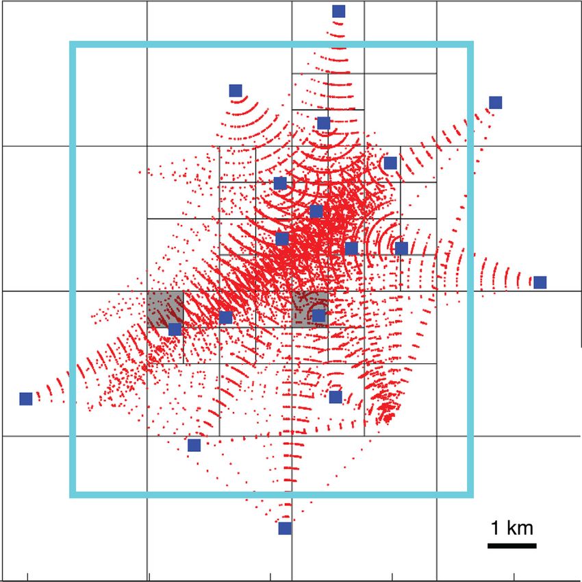
Figure 4. Quadtree grid (black boxes) used to determine the local fast
directions in local regions. Gridding criteria required between 100 and 400
ray paths in each box, with a minimum box size of 750 m. A total of 61 blocks
were used to cover the region encompassed by the LC stations (blue squares).
The red dots show regularly spaced nodes along the ray path between the
station and the source. Polar histograms for the two grey shaded grid cells
are shown in Fig. 5. The cyan box shows the approximate location of the
study area (see Fig. 1).
270 90
fault system was active immediately after the occurrence of the main
shock. We do not observe any apparent growth of the aftershock
zone through time either along strike or with depth.
To examine the temporal evolution of the sequence and density of
events in more detail we divide the main shock fault plane (Profile
C-c in Fig. 7) into grid cells that are 0.5 km by 0.5 km. Of the
grid cells that have at least one event, most of those cells include
an event within the first day after the main shock (Fig. 8a). Over
half (∼59 per cent) of grid cells with at least one earthquake are
180
active for less than 45 d of 3-month catalogue (Fig. 8b). The grid
cells that remain active over much of the study period tend to be Figure 5. (a) Polar histogram for a grid cell that has a single dominant φ
located between the M 4.8 foreshock epicentre to the northeast and apparent in the measurements. This histogram is for a cell located on the
the M 4.8 aftershock epicentre to the southwest, and including the west side of the study area (see west grey shaded box in Fig. 4). (b) Polar
M 5.7 main shock epicentre, remain active through the end of our histogram for a grid cell located near the centre of the study area that has a
catalogue. This same region has the highest density of events with more variable set of φ measurements (see east grey shaded box in Fig. 4).
as many as 538 events occurring in a single grid cell (Fig. 8c). The dashed black bar shows the original TESSA calculation of average φ
Overall, we observe the most prolific families, highest density of (Johnson et al. 2011) and the green bars show up to three principal azimuths
events, and longest active sequences are concentrated in a nest of from the Gaussian peak-fitting method, with length scaled by number of rays
seismicity close the main shock and between the foreshock and that were fit to determine the peak divided by the sum of the rays composing
all of the fitted peaks in the grid cell.
largest aftershock.
We use the expanded catalogue and the FaultID algorithm to de-
termine the set of faults activated in the Prague sequence. The fitted primary planes. The exception is a small fault striking almost per-
faults highlight the three primary rupture planes of the M 4.8 fore- pendicular to the foreshock fault plane towards the northern end
shock, M 5.7 main shock and M4.8 aftershock and 7 minor planes of the sequence that has a shallower dip (071◦ ) than the remaining
(Fig. 9, Supplementary Movie M1). Table 2 and Fig. 9 show the fault planes. The minor fault planes are all within the range of fo-
primary planes agree well with the moment tensor strikes and dips cal mechanisms previously reported (Sumy et al. 2014; McNamara
reported in the Advanced National Seismic System Comprehen- et al. 2015; Walsh & Zoback 2016).
sive catalogue (U.S. Geological Survey 2019) and Global Centroid Given the local stress orientations determined from shear wave
Moment Tensor catalogue (Dziewonski et al. 1981; Ekström et al. splitting, we can determine whether each of the determined fault
2012). The minor fault planes show a range of orientations, with planes is optimally oriented for slip. We assume the stress field re-
the majority having strikes that are subparallel to one of the three mains constant over the duration of the sequence, as suggested by2011 Prague sequence faults and stress 161
(A) (B)
35.6˚ 35.6˚
35.55˚ 35.55˚
35.5˚ 35.5˚
Downloaded from https://academic.oup.com/gji/article/222/1/153/5813439 by guest on 19 September 2020
35.45˚ 35.45˚
km km
0 5 φ regional-aligned 0 5
Primary φ φ regional-rotated
−96.9˚ −96.85˚ −96.8˚ −96.75˚ −96.7˚ −96.9˚ −96.85˚ −96.8˚ −96.75˚ −96.7˚
Figure 6. (a) Principal azimuths (green bars) determined from the Gaussian peak-fitting method plotted at the centre of a grid cell (grid shown in Fig. 4).
The length of each bar is scaled by the number of rays that were fit to determine the peak divided by the sum of the rays composing all of the fitted peaks in
the grid cell. Longer bars indicate a single peak fits most of the measurements. Peaks are only shown if at least 20 measurements contribute to the peak and the
standard deviation of the peak is less than 10◦ . The standard deviations of the azimuths are similar to, or just larger than, the width of the bars and are omitted
for clarity. (b) Unweighted, principal azimuths that most closely aligned with the regional maximum compressive stress direction, N84E from Alt & Zoback
( 2017). Blue bars show the azimuths that are aligned within one standard deviation with the regional stress and red bars shows those that are significantly
rotated. Other symbols are the same as in Fig. 1.
the consistency between the local fast directions and the regional (Casey et al. 2018). Thus, it is critical to understand the occurrence
stress direction (Fig. 6b). It is possible that smaller scale changes of moderate induced earthquake sequences with the hope of better
in the stress occurred that we are unable to resolve with shear wave forecasting future events. Several current forecasting methods use
splitting, however most of the faults we evaluate are similar or larger regional stress field information and orientations of mapped faults
in scale to the resolution of the shear wave splitting estimates. Since in order to predict which structures are more (or less) hazardous in
most of the faults are near-vertically oriented, we assume a 90◦ dip the presence of local fluid disposal (Alt & Zoback 2017; Snee &
and a coefficient of friction of 0.6 such that faults striking 30◦ from Zoback 2018). And, a number of studies show many of the active
the maximum (horizontal) principal stress are optimally orientated structures in Oklahoma are generally optimally oriented in the re-
to slip, similar to the method of Skoumal et al. (2019). Fig. 9 shows gional stress field (McNamara et al. 2015; Walsh & Zoback 2016;
the deviation of individual (100 m long) fault segments from the Schoenball & Ellsworth 2017; Skoumal et al. 2019). However, some
optimal orientation, considering the nearest estimated primary az- studies have suggested slip may sometimes occur on faults that are
imuth with orientation most similar to the regional stress direction unfavourably oriented, at least in the regional stress field (Sumy
(see Fig. 6). We only consider faults with dips within 10◦ from ver- et al. 2014; Skoumal et al. 2019). Here, we determine the local
tical. Faults that have deviations close to zero are optimally oriented stress field and detailed fault sequence of the 2011 M5.7 Prague
for slip, while those with larger deviations are expected to have a earthquake sequence to determine whether the set of activated fault
lower probability of failure. We find that the main shock plane is structures are well oriented for failure.
well oriented for failure across its entire length with deviations from We made 8569 high-quality shear wave splitting measurements
optimal orientation that range from 1◦ to 4◦ . In contrast, the M4.8 (φ, δt) on the temporary stations deployed around the Prague se-
foreshock and M4.8 aftershock fault planes are both unfavourably quence. We find that φ measurements are predominantly oriented
oriented in the local stress field. The M4.8 foreshock fault plane N84◦ E, parallel to the regional principal stress orientation esti-
deviates between 20◦ and 25◦ from the optimal orientation. And, mated from focal mechanism inversions (Sumy et al. 2014; Walsh &
the M4.8 aftershock is more significantly deviated from optimal Zoback 2016). Fracture orientations striking predominantly N75◦ E
orientation, with deviations between 26◦ and 29◦ . were mapped in the upper 60 m in northcentral Oklahoma (Queen
& Rizer 1990), which E. Liu et al. (1991) suggest are oriented close
to the maximum compressive stress direction and may result in
DISCUSSION anisotropic permeability. Thus, we infer that the majority of deter-
Disposal-induced earthquakes, including the 2011 Prague sequence mined φ are sensitive to, and aligned with, the maximum horizontal
in Oklahoma, have in some cases caused damage to structures in the stress. We are unable to constrain stress orientations to a specific
epicentral region (Keranen et al. 2013) as well as concerns about depth range and the variability in measured δt does not allow us
the safety of critical energy infrastructure (McNamara et al. 2015). to constrain the depth extent of the anisotropy. The consistency be-
Further, there may be less immediately visible impacts to local pop- tween φ and the principal stress orientation determined from focal
ulations, including decreased housing prices (Cheung et al. 2018) mechanism inversions, that reflect stresses at source depths, allows
as well as positive correlations of earthquake rates with vehicular us to infer that the stress orientations do not change significantly
collisions (Casey et al. 2019) and Google searches related to anxiety with depth in this region.162 E.S. Cochran et al.
0 Time (days)
0 20 40 60 80
4
0
8
4
C−c
−8 −4 0 4
Downloaded from https://academic.oup.com/gji/article/222/1/153/5813439 by guest on 19 September 2020
35.6˚ 8
B−b
B −2 0 2
c
35.55˚
0
A b
35.5˚
4
a
C
35.45˚
km 8
0 5 A−a
−96.9˚ −96.85˚ −96.8˚ −96.75˚ −96.7˚ −2 0 2
Figure 7. Full catalogue, showing both templates and detections coloured by time in days after the main shock on 6 November 2011 at 3:53:10 in map
and cross-section view. Green and yellow shading in cross-sections shows the approximate depth of the Hunton and Arbuckle Groups. Other symbols are as
described on Fig. 1 .
The dominant azimuths measured from the Gaussian peak fitting et al. 2006; Liu et al. 2008). Here, we do not have sufficient pre-
procedure in most of the grid cells are nearly uniformly, consistent event data to determine whether the orientations change due to the
with the regional stress direction (∼N84◦ E) across the entire study Prague earthquake sequence, but the observed consistency between
area. We observe no significant change in the principal horizontal local and regional stress orientations suggest no significant changes
stress direction for grid cells directly adjacent to the M5.7 main to the stress field occurred. We also see no obvious influence of
shock rupture. The existence or lack of rotations of the principal local injection on the stress orientations at the northeastern end
stress axes following moderate or large ruptures can tell us about of the sequence that has been implicated in triggering (Keranen
the strength of the crust relative to the stress drop of the earthquake et al. 2013). This is in contrast to a study in Kansas that suggested
(Hardebeck & Okada 2018). If the stress drop is of the same order as, temporal rotations in φ resulting from injection (Nolte et al. 2017),
or a large fraction of, the crustal strength then one would expect to although the study does not adequately control for differing source–
see a rotation in fast directions. However, if the stress drop represents receiver paths and their observations may instead reflect spatially
only a small fraction of the total strength of the crust, then no heterogeneous φ. Further, a high-resolution study of anisotropy
such rotation should occur. A few studies have suggested a rotation at a hydraulic fracturing site showed φ remained constant during
of the fast directions following moderate earthquakes measured and after the injection stages, but observed a variation in fracture
from focal mechanism inversions and shear wave splitting (Crampin densities (δt) (Farghal 2018).
et al. 1990; Hauksson 1994). However, as noted by Peng & Ben- In addition to the dominant φ oriented at N84◦ E, we observe a
Zion (2004), extreme care should be taken to ensure that changing subset of fast directions that are parallel to mapped faults or seis-
source–receiver paths are not the cause of an apparent temporal micity lineaments. There is a stronger fault-parallel signature for
change in φ for shear wave splitting studies. Further, several studies grid cells close to the previously mapped Wilzetta fault system (Way
have looked for, but failed to observe, evidence of local changes 1983; Joseph 1987). This may indicate that the Wilzetta fault has a
in fast directions close to recent moderate earthquakes (Cochran more well-developed shear fabric, and thus may be a more mature2011 Prague sequence faults and stress 163
(A) 0 90
80
2 70
First Event (Day)
60
Along Dip (km)
4 50
40
6
30
20
8
10
0
10
-12 -10 -8 -6 -4 -2 0 2 4 6
Downloaded from https://academic.oup.com/gji/article/222/1/153/5813439 by guest on 19 September 2020
Along Strike (km)
0 90
(B)
80
2 70
Last Event (Day)
60
Along Dip (km)
4 50
40
6
30
20
8
10
0
10
-12 -10 -8 -6 -4 -2 0 2 4 6
Along Strike (km)
(C) 0
2 10 2
Event Density (#/km )
2
Along Dip (km)
4
10 1
6
10 0
8
10 10 -1
-12 -10 -8 -6 -4 -2 0 2 4 6
Along Strike (km)
Figure 8. (a) Time in days since the main shock of the first event in each grid cell for cross-section C-c (Fig. 7) divided into 500 m by 500 m cells. (b) Same
as in (a), except showing the time of the last event in each grid cell. (c) Event density (measured in number of events per 500 m by 500 m grid cell) for cross
section C-c.
structure than the southwest portion of the main shock fault. Alter- the three primary rupture planes, so we assume here that the full
nately, the shear wave splitting may be more sensitive to structures in catalogue adequately captures events across these major features.
the sedimentary units, which may suggest the southwestern portion The greatest density of earthquakes is observed to occur where three
of main shock fault does not extend updip into sedimentary groups primary rupture planes of the M4.8 foreshock, M5.7 main shock and
as also suggested by a lack of mapped structures in the region. M4.8 aftershock intersect. In this same active region, the seismicity
The extended catalogue of events provides a high-resolution view extends across the full depth range of the sequence and includes both
of the seismicity over the 90 d following the main shock rupture. the shallowest (∼1 km, in the Arbuckle Group) and deepest (∼10 km
We note that the original catalogue of template events was biased, depth) earthquakes. The area of vigorous seismicity is located where
in that significant attention was given to identifying events in the the mapped Wilzetta system is comprised of a complex set of faults
first 10 d or so after the main shock (see Sumy et al. (2017) for that have been interpreted to act as boundaries to fluid flow (Keranen
details). This initial catalogue includes events distributed across et al. 2013). Way (1983) reports that the Wilzetta fault system is a164 E.S. Cochran et al.
35.6˚
Deviation from Optimal
Orientation (o)
0 15 30 Foreshock
M4.8 Foreshock
(212, 82, 173)
35.55˚
F6
M4.8 Aftershock
(272, 83, −16)
Aftershock
F5 M5.7 Mainshock
(236, 85, −171)
Downloaded from https://academic.oup.com/gji/article/222/1/153/5813439 by guest on 19 September 2020
35.5˚ F4
F2
F3
F1
Mainshock
F7
35.45˚
0 5
−96.9˚ −96.85˚ −96.8˚ −96.75˚ −96.7˚
Figure 9. Fault planes (thick coloured lines) determined by the FaultID algorithm using the full catalogue are coloured by their deviation from the optimal
orientation (◦ ). The optimal fault plane orientation is assumed to be a fault striking 30◦ from the orientation of the local maximum horizontal stress. Local
stress orientations are taken to be the azimuth closest to each 1 km segment of the fault that is most closely aligned with the regional stress direction (green bars
are the primary azimuth with their standard deviations shown by dotted black lines). Note that faults with dips more than ±10◦ from vertical are not assessed
(grey bars). Other symbols are as described in Fig. 1, except here seismicity is shown by open circles here.
Table 2. Fault orientations identified in this study compared with moment are considered unfavourably oriented (Sibson 1990). Keranen et al.
tensors for the M4.8 foreshock, M5.7 main shock and M4.8 aftershock. (2013) suggested the sequence was likely induced due to injection
USGS moment Global centroid into closed fault compartments that caused increased fluid pressures
Fitted plane tensor moment tensors on the foreshock fault. Our finding that the foreshock fault is poorly
oriented may further suggest that elevated fluid pressures may have
Foreshock N31◦ E, 091◦ N32◦ E, 098◦ N27◦ E, 107◦
Main shock N52◦ E, 083◦ N56◦ E, 095◦ N54◦ E, 088◦
induced failure of this structure. The foreshock is subparallel to,
Aftershock N84◦ E, 087◦ N88◦ E, 097◦ N91◦ E, 074◦ and thought to align with, faults along the mapped Wilzetta fault
Fault 1 N48◦ E, 103◦ – – that extends updip into the Arbuckle and Hunton Groups (Way
Fault 2 N84◦ E, 106◦ – – 1983). The observation of fault parallel-aligned fast shear wave
Fault 3 N38◦ E, 077◦ – – orientations is suggestive of shear fabric and may suggest a fault
Fault 4 N25◦ E, 089◦ – – damage zone exists along the Wilzetta fault. Fault damage zones
Fault 5 N44◦ E, 074◦ – – have been shown to have higher permeabilities and may act as
Fault 6 N126◦ E, 071◦ – – conduits for fluid flow parallel to faults (Zhang & Sanderson 1995;
Fault 7 N41◦ E, 096◦ – – Wibberley & Shimamoto 2003). Thus, we surmise that the Wilzetta
fault may have provided a conduit for fluids, leading to increasing
ridge structure comprised of a series of en echelon transverse faults fluid pressure in the Precambrian basement.
rather than a single fracture. Plane fitting to the seismicity also Our results also suggest that the aftershock fault plane is not
suggests a small fault segment subparallel to the main shock fault optimally oriented for slip in the local stress field. Additionally,
plane in this same region. And, to the north, the seismicity appears the static stress changes from the main shock imparted on M4.8
to become sparser past the location of a cross fault that bisects the aftershock epicentre discouraged failure (Sumy et al. 2014). Nor-
foreshock rupture plane. beck & Horne (2016) invoke transient fluid flow resulting in in-
While the M5.7 main shock fault plane is optimally oriented for creased pore fluid pressures to explain the occurrence of the largest
failure in the background stress field, we find that neither the M4.8 aftershock. The penetration of fluid along the eventual plane of
foreshock nor the M4.8 aftershock planes are optimally oriented to the M4.8 aftershock may be supported by observations of pre-
fail in the local stress field with deviations from optimal between 20◦ ceding activity within the damage zone of this structure (Savage
and 29◦ . Faults that deviate more than ±15◦ from optimal orientation et al. 2017).2011 Prague sequence faults and stress 165
The Prague sequence defines ten primary fault planes that have a REFERENCES
wide range of strikes and dips, showing that a heterogeneous set of Alt, R.C. & Zoback, M.D., 2017. In situ stress and active faulting in Okla-
structures were activated in the sequence. Of the five near-vertical homa, Bull. seism. Soc. Am., 107, 216–228.
structures that we evaluate within the context of the regional stress Aster, R.C., Shearer, P.M. & Berger, J., 1990. Quantitative measurements
of shear wave polarizations at the Anza seismic network, Southern Cal-
field, we find that only the main shock and an isolated fault segment
ifornia: implications for shear wave splitting and earthquake prediction,
located in the SE portion of the study area are well-oriented for
J. geophys. Res., 95, 12 449–12 473.
failure. The remaining three structures that host events as large as Balfour, N.J., Savage, M.K. & Townend, J., 2005. Stress and crustal
M4.8 are not optimally oriented to slip. Our results confirm that anisotropy in Marlborough, New Zealand: evidence for low fault
even structures that are not optimally oriented in the regional, or strength and structure-controlled anisotropy, Geophys. J. Int, 163,
local, stress field may host moderate-sized induced events (M∼5). 1073–1086.
Some recent studies have presented assessments of the likelihood Barbour, A.J., Xue, L., Roeloffs, E. & Rubinstein, J.L., 2019. Leakage and
of inducing events based on the orientation of previously identi- increasing fluid pressure detected in Oklahoma’s wastewater disposal
fied faults in the regional stress field, often described as the fault reservoir, J. geophys. Res., 124, 2896–2919.
slip potential (Walsh & Zoback 2016; Alt & Zoback 2017; Snee & Barton, C.A. & Zoback, M.D., 1994. Stress perturbations associated with
active faults penetrated by boreholes: possible evidence for near-complete
Zoback 2018). The activation of unfavourably oriented faults during
Downloaded from https://academic.oup.com/gji/article/222/1/153/5813439 by guest on 19 September 2020
stress drop and a new technique for stress magnitude measurement, J.
the Prague sequence suggests the hazard potential of a given struc-
geophys. Res., 99, 9373–9390.
ture may be difficult to quantify without additional information on Bohnhoff, M., Grosser, H. & Dresen, G., 2006. Strain partitioning and
pre-existing fault stress and hydromechanical considerations. stress rotation at the North Anatolian fault zone from aftershock focal
mechanisms of the 1999 Izmit Mw = 7.4 earthquake, Geophys. J. Int.,
166, 373–385.
Boness, N.L. & Zoback, M.D., 2006. Mapping stress and structurally con-
C O N C LU S I O N S trolled crustal shear velocity anisotropy in California, Geology, 34, 825–
828.
We investigate the 2011 Prague earthquake sequence to determine Booth, D.C. & Crampin, S., 1985. Shear-wave polarizations on a curved
the local principal stress directions, activated fault structures and wavefront at an isotropic free surface, Geophys. J. Int., 83, 31–45.
other characteristics of the sequence. We find that fast orientations Boyd, O.S., McNamara, D.E., Hartzell, S. & Choy, G., 2017. Influence of
measured via shear wave splitting primarily reflect the maximum lithostatic stress on earthquake stress drops in North America, Bull. seism.
horizontal stress direction, with secondary orientations suggesting Soc. Am., 107, 856–868.
the presence of shear fabric aligned subparallel to the Wilzetta Brandon, M.T., 1992. Decomposition of fission-track grain-age distribu-
fault. We find the principal horizontal stress directions are uniform tions, Am. J. Sci., 292, 535–564.
Casey, J.A., Elser, H., Goldman-Mellor, S. & Catalano, R., 2019. Increased
across spatial scales as small as 750 m and are consistent with
motor vehicle crashes following induced earthquakes in Oklahoma, USA,
regional estimates from focal mechanism inversions (Sumy et al. Sci. Total Environ., 650, 2974–2979.
2014; Walsh & Zoback 2016; Alt & Zoback 2017). Casey, J.A., Goldman-Mellor, S. & Catalano, R., 2018. Association be-
We find a majority of aftershocks occur within a 5-km-long por- tween Oklahoma earthquakes and anxiety-related Google search episodes,
tion of the sequence near the M5.7 main shock epicentre that is Environ. Epidemiol., 2, e016, doi:10.1097/EE9.0000000000000016.
bounded to the southwest by the epicentre of the largest aftershock Chen, X. et al., 2017. The Pawnee earthquake as a result of the in-
(M4.8) and to the northeast by the epicentre of a M4.8 foreshock. terplay among injection, faults and foreshocks, Sci. Rep., 7, 4945,
We identify ten distinct fault segments that are activated during the doi:10.1038/s41598-017-04992-z.
sequence. The faults have a wide array of orientations, suggesting Cheung, R., Wetherell, D. & Whitaker, S., 2018. Induced earthquakes and
the activation of a complex fault network. We find that the M5.7 housing markets: Evidence from Oklahoma, Reg. Sci. Urban. Econ., 69,
153–166.
main shock fault is optimally oriented, but both the M4.8 foreshock
Cochran, E.S. & Kroll, K.A., 2015. Stress- and structure-controlled
and M4.8 aftershock occur on fault planes that are deviated from anisotropy in a region of complex faulting—Yuha Desert, California,
the optimal orientation for slip. Our results suggest that elevated Geophys. J. Int., 202, 1109–1121.
pore fluid pressures were likely required for activation of these un- Cochran, E.S., Li, Y.-G. & Vidale, J.E., 2006. Anisotropy in the shal-
favourably oriented planes. This sequence shows that slip can occur low crust observed around the San Andreas Fault before and af-
on faults not well-oriented for failure in the local stress field, and ter the 2004 M 6.0 Parkfield earthquake, Bull. seism. Soc. Am., 96,
care should be taken when forecasting hazard from estimates of S364–S375.
fault slip potential. Cochran, E.S., Ross, Z.E., Harrington, R.M., Dougherty, S.L. & Rubinstein,
J.L., 2018. Induced earthquake families reveal distinctive evolutionary
patterns near disposal wells, J. geophys. Res., 123, 8045–8055.
Cochran, E.S., Vidale, J.E. & Li, Y.-G., 2003. Near-fault anisotropy
following the Hector Mine earthquake, J. geophys. Res., 108,
AC K N OW L E D G E M E N T S doi:10.1029/2002JB002352.
We thank Daniel Trugman for making the GrowClust codes avail- Crampin, S., 1985. Evaluation of anisotropy by shear-wave splitting,
able and providing advice on an appropriate weighting scheme for Geophysics, 50, 142–152.
Crampin, S., Booth, D.C., Evans, R., Peacock, S. & Fletcher, J.B., 1990.
relocation of the template and detected events. We acknowledge
Changes in shear wave splitting at Anza near the time of the North Palm
D. Sumy and C. Neighbors for useful discussions of early SWS
Springs Earthquake, J. geophys. Res., 95, 11 197–11 212.
findings. We thank two anonymous journal reviewers and USGS re- Crotwell, H.P., Owens, T.J. & Ritsema, J., 1999. The TauP Toolkit: flexible
viewers N. Farghal and J. Hardebeck for constructive reviews. The seismic travel-time and ray-path Utilities, Seismol. Res. Lett., 70, 154–
Generic Mapping Tools software was used to generate several of 160.
the figures in this paper (Wessel & Smith 1991; Wessel et al. 2013). Dziewonski, A.M., Chou, T.-A. & Woodhouse, J.H., 1981. Determination of
Any use of trade, firm or product names is for descriptive purposes earthquake source parameters from waveform data for studies of global
only and does not imply endorsement by the U.S. Government. and regional seismicity, J. geophys. Res., 86, 2825–2852.You can also read