Nest choice in arboreal ants is an emergent consequence of network creation under spatial constraints
←
→
Page content transcription
If your browser does not render page correctly, please read the page content below
Swarm Intelligence manuscript No.
(will be inserted by the editor)

Nest choice in arboreal ants is an emergent
consequence of network creation under spatial
constraints

Joanna Chang · Scott Powell · Elva J. H.
Robinson · Matina C. Donaldson-Matasci

Received: date / Accepted: date

Abstract Biological transportation networks must balance competing functional
priorities. The self-organizing mechanisms used to generate such networks have in-
spired scalable algorithms to construct and maintain low-cost and efficient human-
designed transport networks. The pheromone-based trail networks of ants have
been especially valuable in this regard. Here, we use turtle ants as our focal system:
in contrast to the ant species usually used as models for self-organized networks,
these ants live in a spatially constrained arboreal environment where both nesting
options and connecting pathways are limited. Thus, they must solve a distinct
set of challenges which resemble those faced by human transport engineers con-
strained by existing infrastructure. Here, we ask how turtle ant colonies’ choice of
which nests to include in a network may be influenced by their potential to create
connections to other nests. In laboratory experiments with Cephalotes varians and
Cephalotes texanus, we show that nest choice is influenced by spatial constraints,
but in unexpected ways. Under one spatial configuration, colonies preferentially

J. Chang
Department of Biology, Pomona College, Claremont, CA, USA
Tel.: +44 73 8854 6216
E-mail: joanna.chang19@imperial.ac.uk
Present address: Department of Bioengineering, Imperial College London, London, UK
S. Powell
Department of Biological Sciences, George Washington University, Washington, DC, USA
ORCID: 0000-0001-5970-8941
Tel.: +1 202-994-6970
E-mail: scottpowell@gwu.edu
E. J. H. Robinson
Department of Biology, University of York, York, UK
ORCID: 0000-0003-4914-9327
Tel.: +44 1904-328716
E-mail: elva.robinson@york.ac.uk
M. C. Donaldson-Matasci
Department of Biology, Harvey Mudd College, Claremont, CA, USA
ORCID: 0000-0002-9877-384X
Tel.: +1 909-607-1572
E-mail: mdonaldsonmatasci@hmc.edu
2                                                                       Chang et al.

occupied more connected nest sites; however, under another spatial configuration,
this preference disappeared. Comparing the results of these experiments to an
agent-based model, we demonstrate that this apparently idiosyncratic relationship
between nest connectivity and nest choice can emerge without nest preferences via
a combination of self-reinforcing diffusion along constrained pathways and density-
dependent aggregation at nests. While this mechanism does not consistently lead
to the de-novo construction of low-cost, efficient transport networks, it may be an
effective way to expand a network, when coupled with processes of pruning and
restructuring.
Keywords Collective behavior · Transportation network · Self-organization ·
Agent-based model · Arboreal ants · Nest choice

Declarations

Funding This work was funded by NSF award IOS 1755425 (J.C., M.C.D.-M. and
E.J.H.R) and NSF awards IOS 1755406 and DEB 1442256 (S.P.).

Conflicts of interest/Competing interests The authors declare no conflicts of in-
terest and no competing interests, financial or non-financial.

Ethics approval Not applicable

Consent to participate Not applicable

Consent for publication Not applicable

Availability of data and material The data and analyses for the laboratory experi-
ments will be available at https://doi.org/10.5061/dryad.bvq83bk6x upon pub-
lication, and are currently available for review at https://datadryad.org/stash/
share/2uRaUBxkYc_CVtB0kxTxRK-5gEbLA5cUEW-rOjPNxcU. Those for the compu-
tational simulations will be available at https://doi.org/10.5061/dryad.8gtht76n5
and are currently available for review at https://datadryad.org/stash/share/
w8fLUF2FLknioPfj8BJW1L1JVVHBKU90D_0meBd3qcE.

Code availability Code for the model is available at https://github.com/JoannaChang/
TurtleAntSim.

Authors’ contributions All authors contributed to the study conception and de-
sign. J.C. and M.C.D.-M. designed and carried out the laboratory experiments
with input and materials from S.P. The agent-based model was designed by J.C
and M.C.D.-M. with input from E.J.H.R. The agent-based simulations implement-
ing that model were written and run by J.C. Analysis of laboratory and simula-
tion experiments was performed by J.C. and M.C.D.-M. with input from S.P. and
E.J.H.R. The first draft of the manuscript was written by J.C. All authors con-
tributed to subsequent versions of the manuscript, and read and approved the final
manuscript.
Arboreal ant nest choice under spatial constraints                                  3

1 Introduction

Biological transport networks are constructed by many organisms to collect and
distribute vital nutrients. To perform well, a network must be able transport re-
sources efficiently, cost little to construct and maintain, and still remain robust
to disturbances. While biological networks are unable to perfectly optimize all
network features, different biological systems may balance the trade-offs in dis-
tinct ways based on their functional priorities and ecological context. For exam-
ple, leaf venation networks incorporate loops to prioritize dynamic efficiency and
robustness over cost of construction (Katifori et al. 2010), while reconfigurable
Physarum polycephalum slime mold networks prioritize low costs over robustness
(Tero et al. 2010; Reid and Beekman 2013). Polydomous (multi-nest) ant colonies
have become a model system for studying transportation networks because they
frequently move adult ants, brood, and food between multiple spatially separated
nests (Debout et al. 2007). Previous studies on the network structures of sev-
eral polydomous ant species have shown that they are able to construct low-cost
networks that nonetheless achieve relatively high efficiency (Cook et al. 2014; Ca-
banes et al. 2015). Because biological networks like these lack centralized control,
studying the mechanisms used to build such networks has inspired scalable al-
gorithms for constructing and improving human-designed networks that balance
cost, efficiency and robustness in specific ways (reviewed in Perna and Latty 2014;
Nakano 2011). However, these studies have focused on a small handful of biological
systems whose transport networks can expand in two-dimensional space without
spatial constraints.
    Spatial constraints can affect the functionality of both biological and human-
designed transport networks. By restricting where pathways can be built, spatial
constraints can limit the possible connections within a network and affect its ability
to efficiently transport resources and respond to disruptions. For example, leaf ve-
nation patterns are constrained by the 2D plane of a leaf so that veins cannot cross
without intersecting, thereby limiting the routes for nutrient transport through-
out the plant vascular system (Nelson and Dengler 1997). Ant foraging trails are
similarly constrained to the terrain of the ecosystem, limiting the ways food can
be transported back to a colony (Fewell 1988; Cook et al. 2014). Many human-
designed networks also operate under spatial constraints; for example, public tran-
sit networks and power grids need to be built around existing city infrastructure.
Currently, much of the design of human-designed transport networks rely on ap-
proaches based on heuristic algorithms to optimize and balance competing network
properties (Farahani et al. 2013). However, the heuristics need to be constantly
improved, especially in response to changing patterns of demand, and determining
the optimal heuristics proves to be an ongoing challenge (Kepaptsoglou and Kar-
laftis 2009). Studying biological networks which operate under varying degrees of
spatial constraint and translating their local rules into mathematical and compu-
tational models could thus provide useful heuristics to inform the construction of
human-designed networks without the need for centralized planning.
    Polydomous ant species are found in a wide range of ecological contexts, pro-
viding an opportunity to study inter-nest transport networks subject to varying
degrees of spatial constraint. While inter-nest transport networks have been stud-
ied in a variety of distantly related polydomous ant species—including Argentine
ants, Australian meat ants, and European wood ants—they all have large ground-
4 Chang et al.
nesting colonies (Cook et al. 2014; Cabanes et al. 2015). However, polydomy is
also prevalent among arboreal-nesting ants, which are diverse, abundant, and eco-
logically dominant in tropical canopies (Longino et al. 2002; Powell et al. 2011).
Compared to their terrestrial counterparts, polydomous arboreal ants face much
stronger spatial constraints. They are restricted by the topology of the trees they
inhabit, which limits the possible structures of the networks that they construct.
While terrestrial ants can potentially build new trails and nests almost anywhere,
arboreal ants must establish trails along existing tree branches and often only oc-
cupy existing cavities instead of constructing their own nest sites (Carroll 1979;
Powell et al. 2011; Powell 2008). Many arboreal ants never descend to the ground,
and must rely on connecting vegetation to travel beyond a single tree (Adams
et al. 2019). In arboreal networks, decay and strong winds may frequently cause
branches or connecting vines to break, destroying both pathways and nests—which
themselves are already a limited resource (Philpott and Foster 2005; Powell et al.
2011; Gordon 2012). The high risk of these disturbances thus requires arboreal
ants to respond to dynamic environments (Gordon 2017). Conversely, localized
disturbances in terrestrial networks are less disruptive because terrestrial ants are
not constrained to certain physical routes and can more easily re-route around the
disturbances (Oberhauser et al. 2019; Burns et al. 2020). These differences between
the ecological conditions for terrestrial and arboreal ants may lead them to con-
struct networks which balance trade-offs between cost, efficiency and robustness
in different ways. As such, studying arboreal ant networks can provide insight
into the design of transport systems which must continually adapt to changing
conditions, while subject to spatial constraints on both the location of nodes (e.g.
transit stations or nests) and the pathways between them.
In this study, we examined how spatial constraints affect the inter-nest net-
work formation of two arboreal-nesting turtle ant species: Cephalotes varians and
Cephalotes texanus. C. varians are found throughout the mangrove and Hammock
forests of Southern Florida, and especially the Florida Keys (Wilson 1976). C. tex-
anus are typically found in oak trees in southern Texas and northeastern Mexico
(Creighton and Gregg 1954). For Cephalotes, as for many other arboreal ants, vi-
able nest cavities are a limited resource. Cephalotes rely on pre-existing cavities
made by wood-boring beetles (Powell 2008), and differentiate between nests based
on cavity volume and entrance size (Powell 2009; Powell et al. 2017; Powell and
Dornhaus 2013). Cephalotes species that have a soldier caste with a specialized
disc head shape, including C. varians and C. texanus, also tend to occupy cav-
ities with entrance areas that are close to the size of the soldiers’ heads (Powell
2008; Powell et al. 2020). Moreover, Cephalotes colonies tend to occupy nests only
within one tree (Powell 2009), meaning that they are constrained to the nests and
pathways in a single tree. Given that limited nests and pathways impose spatial
constraints on turtle ant networks, this study aims to examine how turtle ants
choose which nests to occupy in constrained spaces where their movement and
options are limited.
Since turtle ant colonies can choose among nests based on intrinsic properties
of the nests themselves, we hypothesized that turtle ant colonies might choose
which nests to occupy based on how they contribute to properties of the network.
First, we conducted two sets of laboratory experiments to determine whether spa-
tial constraints on pathways between nests affect which nests a colony chooses
to occupy. In each set of experiments, we presented turtle ant colonies with anArboreal ant nest choice under spatial constraints 5
environment that had two sections with different spatial constraints: one section
was linearly connected with just a single path connecting the cavities in sequence,
and the other was fully connected with all possible paths between each pair of
cavities (Fig. 1). The ants were given the opportunity to explore both sections
and to move from their original nests into the new cavities in these sections. The
fully-connected section has the potential to form a network with greater efficiency,
greater robustness, and lower cost than the linearly-connected section, so we pre-
dicted that the ants would move into the cavities in the fully-connected section if
spatial constraints influenced nest choice.
Spatial constraints could also affect nest choice indirectly: not as a result of
preference for specific network properties, but as an emergent consequence of the
process of network creation within the spatial constraints of the environment. To
examine this hypothesis, we constructed an agent-based simulation as a null model
to demonstrate how a colony of ants might behave without basing nest preferences
on network properties or making comparisons between nests. Prior models of ant
movement have shown that random walks reinforced with unconditionally laid
trail pheromone allow ant colonies to coordinate movement along specific trails
and choose efficient pathways between existing nests and food sources in a self-
organizing, emergent fashion (Goss et al. 1989; Aron et al. 1990; Dussutour et al.
2004; Ma et al. 2013). However, to our knowledge, the impacts of such a process on
nest choice have not yet been modelled. To model nest choice emerging from spatial
properties alone, we also included a self-reinforcing aggregation rule depending
only on the number of individuals already present. Our model thus explores how
the process of random diffusion coupled with positive feedback loops along paths
and at nests could interact with the spatial constraints of the environment to affect
which nests are occupied.
2 Materials and Methods
2.1 Laboratory Experiments
2.1.1 Study species
Queenright colonies of Cephalotes varians were collected from state-managed Ham-
mock forest in Key Largo, Florida, and queenright colonies of Cephalotes texanus
were collected from live oaks on private property near the city of Gonzalez, Texas.
The first set of experiments, performed in June to July 2017, used three colonies
of C. varians (V1, V2, and V3) and three colonies of C. texanus (T1, T2, and T3).
The second set of experiments, performed in October to November 2017, used four
colonies of C. varians (V4, V5, V6, and V7). The colony sizes (comprising workers,
soldiers, and queens) at the start of each experiment for V1 to V7 and T1 to T3
were 190, 100, 140, 184, 64, 137, 56, 43, 55, and 82, respectively.
2.1.2 Experimental setup
To examine how spatial constraints affect turtle ant nest choice, we constructed
arenas that had two sections with different structural features and levels of con-
straint (Fig. 1). One section had cavities that were fully connected to one another6 Chang et al. a) b) c) Fig. 1 Arena setups for laboratory experiments. Arenas were made of boxes connected by arched bridges. Rectangles within the boxes represent nest cavities. Each arena had 2 sections: one with fully connected cavities (F, orange) and one with linearly connected cavities (L, blue). Original cavities were put in at (O), equidistant from the closest cavities in F and L. Circles represent food and water. a) Diagram of the limited-cavity setup; b) Diagram of the additional-cavity setup; c) Picture of the limited-cavity setup with outlines drawn in for the F and L sections. (F), while the other section had cavities that were linearly connected in sequence (L), with greater distances between the cavities. The F section had cavities that were closer to each other with more possible pathways between them, so it was less constrained than the L section. The arenas were made with boxes (dimensions: 11 x 11 x 3.75 cm high) in a grid arrangement as shown in Fig. 1. Boxes were con- nected with arched paper bridges which went from the floor of one box to the floor of another, over their adjacent walls. Fluon was applied to the sides of each box to prevent ants from escaping. The artificial nest cavities all had the same entrance size and volume and were made as outlined in Powell and Dornhaus (2013). In the first set of experiments (June to July 2017), there were three nest cavities in each section for a total of six cavities while in the second set of experiments (October to November 2017), there were four nest cavities in each section for a total of eight cavities (Fig. 1). Additional cavities were added in the second set of experiments to allow us to assess potential nest preferences in larger colonies that may be finding and occupying all of the cavities. For the rest of this paper, the two sets of experiments will be referred to as the limited-cavity and additional-cavity experiments, respectively. 2.1.3 Nest Choice Experiments At the beginning of each experiment, we placed original cavities containing a single turtle ant colony in the box labeled O, equidistant from the closest cavities in the F and L sections (Fig. 1). We then opened the original cavities to force the ants to move and occupy new cavities in the arena. Colony movement was filmed for the first 12 hours and cavity occupation was checked 4 times a day at 8:00, 12:00, 16:00, and 20:00. Cavity occupation was measured by lifting the outer cover of the cavities and counting the number of workers inside with minimal disturbance. Both workers and soldiers moved between cavities, but workers were counted for simplicity and because they were much more numerous. The presence of brood was also noted. Turtle ants rapidly allocate workers and brood to new cavities and differentiate between different cavity properties (Powell and Dornhaus 2013), so both the number of workers occupying a cavity and the presence of brood can be used as indications of their preference for the cavity. The limited-cavity experiments lasted 5 days and showed that colonies occupied new cavities within
Arboreal ant nest choice under spatial constraints                                  7

the first 12 hours, with the proportions of ants in each cavity remaining stable
after the second day. Thus, the additional-cavity experiments lasted only 3 days.

2.2 Simulation Modeling

2.2.1 Model Description

The model description follows the ODD (Overview, Design concepts, Details) pro-
tocol, a standardized structure for describing agent-based models (Grimm et al.
2006, 2010).

Purpose This agent-based model simulates the movement and cavity occupation
of an ant colony within a constrained space that can be designed by the user.
The space (or arena) may have different structural features based on the spatial
arrangement of the cavities and the bridges between them. This model is designed
to explore the effects of structural constraints on turtle ant cavity occupation
when the ant agents act under simple rules of movement driven by diffusion and
pheromone feedback loops on trails and at nests, excluding preference or memory.
Specifically, we used this model to examine the cavity occupation in simulated
arenas based upon the two arenas used in the laboratory experiments described
above. Within each arena, we compared the cavity occupation between two sections
with different spatial features. Between the two arenas, we examined how the
proportional occupation of these two sections differed.

Entities, State Variables, and Scales The agent-based model has two kinds of
entities: ant agents and square cells. The ant agents represent the individuals of
an ant colony that participate in exploration for new cavities, and there are 100
agents in each simulation. Each agent has a unique ID used to track its individual
movement and two state variables to track its orientation and location (described
as the cell that it is on). A 2D grid represents the floor of the arena and is divided
into square cells. Arched bridges exist outside of the grid and are also made up of
square cells. The length of a cell corresponds to the length of a worker ant, which is
about 4.5 mm for the turtle ant species we used (C. varians and C. texanus). Each
cell can represent either a wall, a cavity, a bridge, or an empty space (Fig. 2). The
type of each cell is determined by the user based on the design of the arena. Each
cell has two state variables that track the amount of pheromone and the number
of ant agents in the cell. Empty cells within the arena may also have access to
a bridge; such cells, called bridge accessor cells, represent the ends of the bridge
where agents can get onto the bridge. Each bridge is made of an array of bridge
cells and two bridge accessor cells at the ends of the array; this array is flanked
on both sides by arrays of wall cells (representing the boundaries of the bridge)
(Fig. 2c).

Initialization The structure of the arena, designated by the positions of each cell
type, is generated when the simulation starts. The structure depends on user
input: in this study, we ran simulations with two different structures modeled
after arenas from laboratory experiments (Fig. 2). All of the cells are initialized
without any pheromones. One hundred ant agents, each facing a random direction,
8                                                                                    Chang et al.

a)                        b)                          c)

                                                           Ant     Bridge accessor
                                                           Nest    Bridge
                                                           Empty   Wall

Fig. 2 Arena structures for the agent-based model. Cells in the arena can represent a
wall, a nest cavity, a bridge, or an empty space; they make up the 2D grid representing the
floor of the arena and the bridges that exist outside of the grid. Empty spaces that have access
to a bridge are bridge accessor cells. Ant agents are generated within a random area designated
by the starting location. a) Floor of the arena structure (excluding the bridges) modeled after
the limited-cavity setup; b) Floor of the arena structure (excluding the bridges) modeled after
the additional-cavity setup; c) A bridge of length 5 consisting of two bridge accessor cells and
5 bridge cells, flanked on both sides by wall cells.

are generated in random cells within a 10 x 10 grid of cells surrounding a starting
location.

Process Overview and Scheduling Each time step represents the amount of time
an ant takes to traverse the length of a cell (i.e. its own body length) and is
approximately equal to 1 second of real time. During each time step, each ant
agent has a probability of turning and a probability of moving into a new cell
(the details of movement are outlined under “Movement Submodel”). Agents that
move into a new cell or stay in a cavity deposit pheromone into the cell (details
under “Pheromone Submodel”). The movements for each agent are tracked by
recording each time it enters or exits a cavity or crosses a bridge. The order of
ant agent movement is randomized within each time step so that the effect of an
agent’s movement on subsequent agents is randomized. After all of the agents have
moved within the time step, the amount of pheromone in each cell is decreased.
Each simulation lasts for 50,000 time steps, which is approximately equal to 14
hours and encompasses the initial stages of exploration according to the empirical
experiments. At the end of each simulation, the number of agents in each cavity
is recorded.

Design Concepts The basic principle addressed by this model is the concept of
spatial constraints and how they may affect ant occupation in nest cavities by lim-
iting possible network structures. In particular, the model examines how apparent
nest preferences—examined as ant occupation in different cavities—can emerge
from the movement of ant agents through cells that make up a constrained space
(the arena). This behavior is modeled dynamically as the ant agents sense and re-
act to changes in the amount of pheromone in adjacent cells, and interact with the
cells by depositing pheromones. While this behavior is consistent with an adaptive
response—ants tend to follow pheromone trails that can increase their fitness by
leading to resources like food and nest cavities—ant agents in the simulation have
no defined goals and lay pheromones unconditionally; the model thus explores how
ants behave when they are solely driven by pheromones, and not by other factors
that may maximize fitness (Goss et al. 1989; Deneubourg et al. 1990).
Arboreal ant nest choice under spatial constraints 9
Stochasticity is used to represent variability in ant movement. Ant agents usu-
ally move in a forward direction and follow stronger pheromone trails, but they
also sometimes turn or explore new paths (Garnier et al. 2009; Chandrasekhar
et al. 2018). Ant agents aggregate in cavities according to a positive feedback
loop, where the chance of an ant agent leaving a cavity decreases exponentially
as the number of ants within the cavity increases (Deneubourg et al. 2002). In
this study, we used pheromones to model local positive feedback loops at nest
cavities, but such feedback loops could take different forms for real ant colonies
(Pratt 2005). Additional details about movement and pheromones are outlined in
“Movement Submodel” and “Pheromone Submodel”, respectively.
Throughout the simulations, agent movement is observed by recording entries
into and exits from cavities, as well as crossings over bridges. At the end of the
simulations, cavity occupation is observed as the total number of agents in each
cavity.
Movement Submodel The movement submodel defines how ant agents move within
the arena according to a diffusion process and pheromone-mediated positive feed-
back loops. Many species of real ants, including turtle ants, deposit chemical
pheromones which can be detected by other ants within a colony (Wilson 1976).
Ants following a trail of pheromones can also deposit their own pheromones, creat-
ing a positive feedback loop along the trail. Turtle ants usually move in a forward
direction and presumably follow stronger pheromone trails, but they also have
high rates of movement and exploration on new paths (Gordon 2017).
Ant agent movement is summarized in Fig. 3. If an agent is in a cavity at
the beginning of its move, it has a probability of leaving the cavity calculated
by qexit /2(pn +an )/py . The parameter pn is the amount of pheromone in the nest
cavity; an is the parameter nest cavity attractiveness, which is used to model
the greater likelihood that an ant will explore a cavity compared to an empty
space. The probability of leaving a cavity decreases with more pheromone in the
cavity; the parameter py (the staying factor ) refers to the amount of pheromone
that decreases this probability by half. The value of the parameter qexit is 0.5,
meaning that the agent has an equal probability of staying or leaving the cavity
in the absence of pheromone and when cavity attractiveness is zero. If the agent
leaves the cavity (or if it is not in a cavity to begin with), it has a probability of
turning determined by the parameter qturn . If it turns, it does so within a uniform,
symmetric range of degrees (e.g. -90 to 90 degrees) determined by the parameter
turning range. From the new direction it is facing, the agent can perceive any
adjacent non-wall cells within its field of vision, determined by the parameter
vision range. Agents on bridge accessor cells can also perceive the first empty cell
on a bridge, regardless of the direction they are facing. The agent then stays in its
current cell or moves to any of the cells it can perceive based on a weighted random
walk. The weight of any adjacent cavity cell, if present, is ac + an + pc , where ac
is the parameter cell attractiveness, an is the parameter nest cavity attractiveness,
and pc is the amount of pheromone in the cell. The weight of non-cavity adjacent
cells is ac + pc and the weight of the current cell is ac because an agent is not
following a pheromone trail by staying in place. Cell attractiveness refers to the
intrinsic attractiveness of each cell and allows neighboring cells with no pheromone
to be considered in the weighted random walk. If an agent moves onto a bridge10 Chang et al.
1 2b 3b 4b
?
?
2a 5b 6b 7b
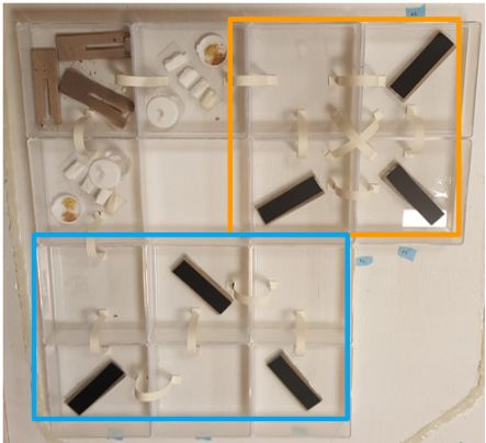
Fig. 3 Ant agent movement. 1) Ant agents in a cavity (blue) have a probability of leaving.
2a) If they stay, they deposit pheromones in the cavity. 2b) If they leave a cavity or if they were
originally not in a cavity, they have a probability of turning. 3b) If they turn, they randomly
turn within a turning range. 4b) After turning, they can perceive adjacent cells within a vision
range. They can move into any cell within their range of vision or remain in their current cell.
5b) They take their next step based on a weighted random walk, where each adjacent cell is
weighted by the amount of pheromone (pink ) it contains. Cavity, non-cavity, and current cells
are weighted differently. If they move into a new cell (6b), they deposit pheromone into it (7b).
cell, it traverses the cells of the bridge according to the same rules of movement
as those in the rest of the arena.
Pheromone Submodel The pheromone submodel defines how the amount of pheromone
is updated as a state variable for each cell. Each time an agent enters a new cell, it
increases the pheromone value by depositing an amount of pheromone determined
by the parameter pheromone strength (ps ). Agents that remain in cavities also de-
posit pheromone in each step. The amount of pheromone in each cell is saturated
at the parameter max pheromone (pm ). After each time step, the pheromone in
each cell is decreased exponentially by the rate qdecay to model the decay of real
pheromones over time.
Simulation Experiments and Data Collection The model was implemented in Java
8 and each experiment had 100 simulations (Table 1). Each simulation ran for
50,000 time steps, with each time step equal to 1 second. To examine how spatial
constraints might have affected turtle cavity occupation in our laboratory exper-
iments via limited diffusion and pheromone feedback loops, we ran experiments
with arena structures based on the limited-cavity and additional-cavity arenas
(Figs. 1 & 2). We performed preliminary analyses to determine and validate the
parameters that modeled ant movement (Online Resource 1). To further exam-
ine the effects of pheromones on ant movement, additional simulations were run
that 1) removed all pheromones from the model and 2) modeled pheromones only
within cavity cells (Fig. 7). Apart from varying the arena structure and pheromone
presence, all of the experiments used the parameters outlined in Table 1. During
each simulation, the time step and ant ID for each bridge crossing, cavity entrance,
and cavity exit were recorded. At the end of each simulation, the number of ant
agents in each cavity was recorded.Table 1 Model Parameters
Description Parameter Value Rationale/notes
Arena Structure: includes locations of each type of – varied (Fig. 2) based on laboratory experiments
cell, locations of bridges, and bridge lengths
Starting position – middle of original box agents are generated within 5 cells of this location
Number of ant agents – 100 approximate size of colonies in laboratory experiments
Number of time steps – 50,000 equal to 14 hours real time
Max pheromone in a cell pm 550 validated in Supplemental Materials
Pheromone strength: amount of pheromone deposited ps 4 validated in Supplemental Materials
by an agent
Staying factor: amount of pheromone that decreases py 50 validated in Supplemental Materials
the probability an ant agent will leave a cavity by half
Nest cavity attractiveness: additional attractiveness an 8 validated in Supplemental Materials, represents the
of a cavity compared to an empty cell greater likelihood an agent will explore a nest cavity
Arboreal ant nest choice under spatial constraints
over an empty space
Cell attractiveness: intrinsic attractiveness of a cell ac 12 allows all potential cells to be considered within a move
Probability of turning qturn 0.2 consistent with Chandrasekhar et al. (2018), validated
in Supplementary Materials
Baseline probability of exiting a cavity without ac- qexit 0.5 no bias for staying or leaving a cavity without
counting for pheromones or attractiveness pheromones or attractiveness
Pheromone decay per time step (%) qdecay 0.05 consistent with Chandrasekhar et al. (2018)
Turning range: maximum possible turn (degrees) – -90 to 90 prevents agents from going backwards in one step; con-
sistent with Sendova-Franks and Lent (2001) and Perna
et al (2012)
Vision range: field of vision (degrees) – -90 to 90 prevents agents from going backwards in one step, de-
termines where agents can move
1112 Chang et al.
2.3 Statistical analyses
We used generalized linear mixed models to examine turtle ant occupation across
the different cavities at the end of each laboratory experiment. We used a Poisson
distribution to model the number of worker ants in each cavity, and a binomial
distribution for the presence of brood in each cavity. Within each model, the
colony was included as a random effect to account for consistent differences be-
tween colonies. The observation identifier (a unique identifier assigned each time
occupation was counted for each cavity) was used as an additional observation-
level random effect to account for overdispersion caused by the possibility that
ants aggregate non-independently in cavities (Harrison 2014). The cavity connec-
tivity (whether a cavity was in section F or L) was included as a fixed effect since
we were interested in the effects of structural features on cavity choice. For the
model of number of worker ants per cavity, we also included species (C. varians
or C. texanus) as a fixed effect, to account for consistent differences in colony size
between species.
We also used randomization tests to examine whether the observed effects of
structural features on cavity occupation could have been due to chance. First,
we chose just to consider the observation in the afternoon of the third day as
being representative of the colony decision. The number of ants was averaged
across all cavities in each section (F and L) for each colony, and the test statistic
was calculated as the difference between the two sections, averaged across all
colonies in each experiment. In each randomization, the section label for each
cavity (F or L) was randomly shuffled within each colony, and the test statistic
was recalculated. For each experiment, 5000 randomizations were performed to
calculate the proportion of randomizations with test statistics more extreme than
the observed test statistic.
3 Results
3.1 How do spatial constraints affect turtle ant nest choice?
We examined turtle ant cavity occupation in the laboratory experiments by ob-
serving the numbers of workers and the presence of brood in each section (the
fully-connected section or the linearly-connected section) at the end of each ex-
periment (Fig. 4). In the limited-cavity experiments, there was significantly greater
occupation of the fully-connected section than the linearly-connected section based
on the total number of workers (Poisson GLMM, effect = 1.12 ± 0.44, p = 0.01)
and the presence of brood (Binomial GLMM, effect = 3.66 ± 1.49, p = 0.01) in
each cavity. On average, colonies had 11.27 more ants per occupied cavity in the
fully connected section than in the linearly connected section. Out of 5000 ran-
domizations, none yielded such a large difference between the sections. However,
there was no significant difference in cavity occupation between the two sections in
the additional-cavity experiments, neither based on the number of workers (Pois-
son GLMM, effect = 0.14 ± 0.55, p = 0.80) nor the presence of brood (Binomial
GLMM, effect = −6 × 10⁻⁷ ± 4.6, p = 1.0). The randomization test also showed
no significant effect: the experimental colonies had just 1.06 more ants per cavity
in the fully connected section on average, and over a third (1941 out of 5000) ofArboreal ant nest choice under spatial constraints 13
a) b)
Fig. 4 Final cavity occupation is affected by spatial constraints. The number of
workers per cavity was observed at the end of each empirical experiment for each colony in the
a) limited-cavity setup and b) additional-cavity setup. In the limited-cavity setup, there were
always more workers in the fully connected (F) cavities, while in the additional-cavity setup
only half the colonies had more workers in F cavities.
the randomizations yielded a difference between sections that was greater. While
colonies in the two sets of experiments had different patterns of cavity occupation,
they had similar levels of activity, with the same number of cavities found and
occupied within the first 8 hours (Fig. 5).
Each colony typically occupied most of the cavities; however, instead of dis-
tributing workers evenly across the cavities, all colonies except for T3 (the smallest
colony) either concentrated most of their workers into just one cavity, or split most
of their workers between two cavities within the first day of the experiments. These
cavities had at least 2.5 times as many ants as any other cavity at the end of the
experiments, and they typically had most, if not all, of the brood and soldiers.
We thus take these criteria as an indicator of cavity choice. In the limited-cavity
experiments, all of the colonies except for T3 (Fig. 5c) chose to aggregate in one
cavity, and it was always in the F section (e.g. Fig. 5a & 5b). In the additional-
cavity experiments, all of the colonies chose to aggregate in F1, L1, or both (e.g.
Fig. 5d, 5e and 5f). All of the chosen cavities were among the closest available
cavities to the original cavities (limited-cavity experiment: F1, F2, F3 and L1;
additional-cavity experiment: F1 and L1) (see Fig. 1).
3.2 Could spatial constraints indirectly affect nest choice?
While the empirical results for the limited-cavity setup seem to suggest a prefer-
ence for well-connected nests, the empirical results for the additional-cavity setup
do not. As an alternative, we hypothesized that nest choice could be indirectly
influenced by spatial constraints, emerging from movement patterns within those
constraints, even in the absence of preference. To test this hypothesis, we created
a model for ant movement through arena structures based on the experimental se-
tups. The model simulates ant movement based on simple diffusion, self-reinforcing
movement, and density-dependent aggregation at nests, without preferential re-
cruitment to specific nests. By varying the parameters controlling how many ant
agents are needed to induce others to stay at a nest, the model can generate a14 Chang et al.
a) b) c)
d) e) f)
Fig. 5 Ants were concentrated in one or two nest cavities. Within the first day of
the empirical experiments, all colonies had concentrated most of their workers and brood into
just one or two nest cavities and the trends in occupation remained the same after the first
day (except for T3). Colonies in the limited-cavity experiments typically chose to aggregate
in one cavity in F. Two examples are shown: a) Colony V2, b) Colony T1. An exception was
c) Colony T3. Colonies in the additional-cavity experiments chose to aggregate in F1, L1, or
both. Three examples are shown: d) Colony V5, e) Colony V6, f) Colony V7.
variety of results, ranging from consensus choice of one nest to dispersion across
all of them (see Online Resource 1). We chose parameter values to produce levels
of aggregation similar to those observed in the laboratory experiments: simulated
colonies typically occupied one or two cavities (i.e., they aggregated in one or two
nests, containing at least 2.5 times as many ants as any other nest). Under these
conditions, as observed empirically, the cavities closest to the starting positions
(L1 and F1-3 for the limited-cavity experiments and L1 and F1 for the additional
cavity experiments) were more likely to be occupied (Fig. 6). Thus, the majority
of simulations fell into one of three categories: (1) most ant agents aggregated in
one nest in F, (2) most ant agents aggregated in one nest in L, or (3) the group
split between two nests, one in each section (Fig. 6).
The simulations showed that patterns of cavity occupation similar to those
observed in the laboratory experiments could emerge without being driven by
preference. Like the laboratory results, the simulation results showed greater usage
of nests in the fully-connected section for the limited-cavity experiments, but not in
the additional-cavity experiments. In the limited-cavity experiments, simulations
were 5.9 times more likely to fall in the ‘Single nest in F’ category than in the
‘Single nest in L’ category, and there were few cases of splitting between F and L
(Single nest in F: 59, Single nest in L: 10, Split between F and L: 9, out of 100
simulations). In contrast, in the additional-cavity experiments, simulations were
1.5 times more likely to fall in the ‘Single nest in L’ category than in the ‘Single
nest in F’ category, and the majority of simulations had splitting between F and
L (Single nest in F: 16, Single nest in L: 25, Split between F and L: 52, out of 100Arboreal ant nest choice under spatial constraints 15
a) b)
Category Category
Single nest in F Single nest in F
Single nest in L Single nest in L
Split F & L Split F & L
Other Other
Cavity Cavity
L1 L1
L2 L2
L3 L3
F1 L4
F2 F1
F3 F2
F3
F4
Fig. 6 Cavity occupation patterns were different under different spatial con-
straints. Cavity occupation was recorded at the end of each simulation for the a) limited-cavity
arena structure and b) additional-cavity arena structure. Each simulation was assigned to one
of 4 categories according to where most ant agents aggregated at the end of the simulation:
(1) Single nest in F; (2) Single nest in L; (3) Split between F and L; and (4) Other if the
simulation did not fit into any of those categories.
simulations). These patterns remained robust across a range of suitable parameter
values (Online Resource 1).
3.3 How do spatial constraints mechanistically drive patterns in cavity
occupation?
To understand the mechanisms that drive patterns in cavity occupation, we ex-
amined the distribution and movement of the simulated ants within the spatial
structures. In both the additional-cavity and limited-cavity experiments, the pro-
portions of ant agents in the boxes of each section were about 50-50, but the
proportions of ant agents in the cavities of each section differed between the ex-
perimental setups (Fig. 7a). This difference suggested that the agents diffused
equally into the boxes of the linearly-connected and fully-connected sections, but
moved into the cavities in proportions which differed between the experiments.
To parse out the effects of diffusion and pheromone feedback loops on move-
ment, we ran two additional sets of experiments: one without any pheromones
to model the effects of diffusion alone, and one with pheromones deposited only
within nest cavity cells to model the effects of diffusion plus local pheromone feed-
back loops at cavity cells. In the set without any pheromones, the rate of ant
agents encountering each cavity reflected cavity occupation distribution patterns
observed in both the laboratory and simulation experiments. Encounter rate was
highest for the three F cavities in the limited-cavity experiments while it was
highest for the L1 cavity, then the F1 cavity, in the additional-cavity experiments
(Fig. 7b); these were the most populated nests in the respective laboratory experi-
ments (Fig. 5) and simulation experiments (Fig. 8c & 8f). Thus, diffusion alone can
explain the overall distribution of ants in the experiments. However, pheromones
are still necessary for ants to accumulate in cavities. In the set of simulations with
pheromones only within cavity cells, the limited-cavity and additional-cavity ex-
periments showed similar proportions of ant agents in the boxes of each section but
dissimilar proportions of agents in the cavities of each section, just as in the exper-
iments with pheromones in all cells (Fig. 7a). Therefore, the observed patterns in16 Chang et al.
a) b)
Fig. 7 Simulation results showing cavity occupation depends on cavity encounter
rates driven by diffusion and local pheromone feedback loops at cavity cells. a)
Between the additional-cavity and limited-cavity experiments, the proportions of ant agents
in the cavities of each section were similar, but the proportions of agents in the boxes of each
section were dissimilar. b) In diffusion-only (no pheromone) experiments, patterns in encounter
rates for each cavity reflect patterns of cavity occupation, with higher rates corresponding to
greater occupation.
cavity occupation can be achieved with diffusion driving ant movement outside of
cavity cells and with local pheromone feedback loops driving ant movement within
cavity cells.
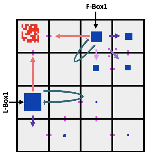
Proximity to the cavity cells is required for ant agents to be affected by local
pheromone feedback loops, so we examined how spatial features can lead agents
to encounter or bypass cavity cells through diffusion. Specifically, we examined
the behavior of the ant agents when they first enter the two structurally different
sections through the boxes closest to the original cavity: L-Box 1 and F-Box 1
(Fig. 8a & 8d). The paths leading to these two boxes from the original cavity are
exactly equivalent, but the paths leading onward are different, so this was a good
place to look for sources of asymmetry between the two sections. Also, the only
difference between the F sections in the limited-cavity and additional-cavity arena
structures was the addition of a cavity in F-Box 1, making that box of particular
interest. We thus inferred that the spatial structure surrounding F-Box 1 likely
contributed to the differences observed between the experiments, and we focused
on how ant agents moved at F-Box 1 and its equivalent in the other section, L-
Box 1. Specifically, we documented the movement of ant agents after they entered
F-Box 1 or L-Box 1 and categorized their next steps as ‘backward’ (moving back
towards the original nest), ‘forward’ (moving forwards into the section), or ‘nest’
(going into a nest cavity in the box) (Fig. 8).
In both the limited-cavity and the additional-cavity experiments, additional
forward paths in F-Box 1 compared to L-Box 1 caused greater forward move-
ment into the fully-connected section compared to the linearly-connected section.
In both setups, there were three forward paths from F-Box 1, compared to one
forward path in L-Box 1. As such, there was a greater or equal proportion of ant
agents moving forwards than backwards from F-Box 1, compared to a smaller
proportion of ants moving forwards than backwards from L-Box 1 (see Fig. 8b &
8e). While these patterns of movement are similar between the limited-cavity and
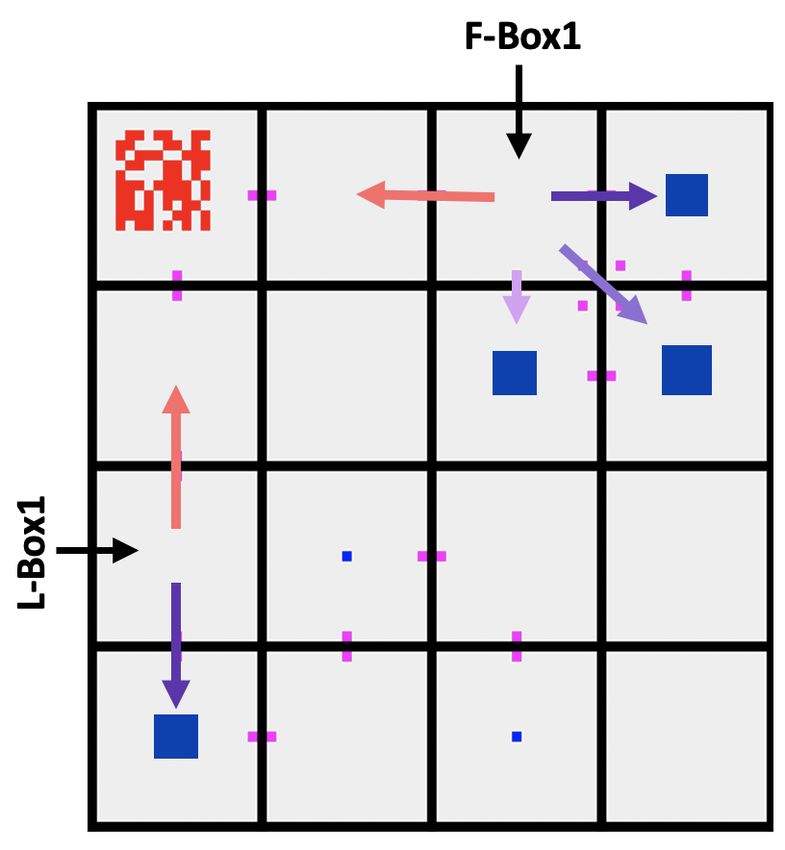
additional-cavity experiments, they have different effects on cavity occupation. InArboreal ant nest choice under spatial constraints 17 a) b) c) a) b) c) Fig. 8 Simulation results showing greater forward movement from F-Box 1 com- pared to L-Box 1. The movement of ant agents once they entered the first box of each fully-connected (F) or linearly-connected (L) section was examined and their next steps were categorized as ‘backward’ (moving back to the original cavity), ‘forward’ (moving forward into the section), or ‘nest’ (going into a nest cavity in the box). Proportion of agents that took each type of step for all simulations in the a) limited-cavity arena structure and d) additional-cavity arena structure. Average proportion of agents that took each step for the b) limited-cavity arena and e) additional-cavity arena. Summary diagram of movement in the c) limited-cavity arena and f) additional-cavity arena. Size of blue cavities is proportional to average number of agents in the cavity at the end of all simulations, and length of arrows indicates relative proportion of agents that take the step. the limited-cavity experiments, greater forward movement from F-Box 1 results in less backward movement, compared to L-Box 1 (Fig. 8b). This led to greater occu- pation in the fully-connected section, likely by allowing more agents to encounter the three F cavities that are equidistant from the original cavity (Fig. 8c). How- ever, in the additional-cavity experiments, greater forward movement from F-Box 1 causes agents to miss the closest F nest in F-Box 1 without affecting the rate of backward movement, compared to L-Box 1 (Fig. 8e). This led to less occupation in the fully-connected section, likely by reducing the rate of encounter at the closest F nest (Fig. 8f). 4 Discussion Our empirical results show that spatial constraints can affect turtle ant nest choice and thus shape the formation of their transport networks. In two sets of experi- ments designed to test whether colonies would preferentially occupy different phys- ically equivalent nests based on network characteristics, we observed apparently conflicting results. The experiment with fewer cavities suggested a preference for nests with close connections to other nests, but the experiment with additional cavities did not. Taken alone, these empirical results might suggest that turtle ant
18                                                                       Chang et al.

colonies preferentially target well-connected nests, but only under specific condi-
tions. One explanation for the observed differences could be changes in activity
level or motivation during the different seasons in which the two sets of exper-
iments were performed, which have been observed in other species (Heller and
Gordon 2006; Stroeymeyt et al. 2014). However, colonies in the two sets of exper-
iments showed similar patterns of exploration and occupation, both in terms of
numbers of active ants and nests occupied. More importantly, simulations of ant
movement based on the two sets of experiments show that the observed patterns
can in fact be explained as an emergent consequence of simple rules of diffusion and
pheromone feedback loops, interacting with subtle differences in the layouts of the
two experimental set-ups. Since the computational simulations do not model pref-
erence or memory, the results demonstrate that the empirically observed patterns
of nest choice could emerge from the imposed spatial constraints, even without
individual preference for nests that improve network characteristics of efficiency
and robustness.
    Our model of nest choice focuses on emergent effects of spatial constraints
by including only quality-independent feedback processes: continuous trail-laying
outside the nest, and density-dependent aggregation inside the nest. Classic mod-
els of nest choice in social insect colonies utilize quality-dependent recruitment
coupled with a quorum threshold rule to balance three objectives: speed, accuracy
and group cohesion (Sumpter and Pratt 2009). In the two best-studied examples,
rock ants and honey bees, individuals assess site quality directly, judging char-
acteristics like cavity volume and entrance size; quality-dependent recruitment
then amplifies traffic to the best site more quickly than to other sites, allowing
the group to integrate information collected by many individuals and make ac-
curate consensus decisions (reviewed in Franks et al. 2002). We know that turtle
ant colonies also choose to occupy cavities based on physical nest properties like
entrance size (Powell 2009; Powell et al. 2020) and cavity volume (Powell and
Dornhaus 2013). Besides quality-dependent recruitment, such preferences could
emerge from quality-dependent resting time at a nest, as in cockroaches aggregat-
ing at a shelter (Jeanson et al. 2007), or even a combination of the two, as observed
in the ant Messor barbarus (Jeanson et al. 2004). While our work does not rule out
the possibility that nest choice is influenced by individual ants assessing the spa-
tial characteristics of physically equivalent nests, it demonstrates that nest choice
can be influenced by spatial characteristics in an emergent fashion, even without
such assessment. How the interactions play out between the emergent spatial in-
fluences on nest choice and the demonstrated preferences for certain physical nest
properties remains to be explored.
    Of the two quality-independent feedback processes we included, trail-laying
outside the nest might seem a natural candidate to produce indirect spatial ef-
fects on nest choice. Argentine ants use continuous trail-laying to choose shorter
paths, leading to efficient and low-cost networks of trails linking multiple pre-
established nests (Goss et al. 1989; Aron et al. 1990; Latty et al. 2011). Although
nothing is known about pheromone use in C. varians or C. texanus specifically,
it has been suggested that Cephalotes goniodontus may also lay pheromone con-
tinuously, allowing colonies to improve efficiency of foraging trails (Gordon 2017;
Chandrasekhar et al. 2018). If so, we might expect this process to impact turtle
nest choice during colony expansion into new cavities, potentially leading to the
construction of efficient and low-cost networks. However, we found that simulated
Arboreal ant nest choice under spatial constraints 19
colonies, like real turtle ant colonies, did not always choose sets of nests leading to
an efficient, low-cost network. Furthermore, since qualitatively similar results were
observed with and without pheromones outside the nest, we can conclude that pos-
itive feedback along trails is not necessary to explain the qualitative patterns of
nest choice we observed.
Instead, the patterns of nest choice we observed in the simulations seem to
be driven primarily by the second positive-feedback loop—aggregation at the
nest—interacting with the diffusive flow of ant agents along constrained pathways.
To induce aggregation at the nest, we included a quality-independent positive feed-
back rule based only on the number of individuals already present, as has been
suggested for other gregarious invertebrates choosing a shelter without spatial
constraints (e.g. Ame et al. 2004; Broly et al. 2016). This induces a quorum-type
response, allowing us to represent a continuum of strategies—ranging from perfect
consensus to dispersion across all nests—by varying the parameters controlling
how many ant agents are needed to induce others to stay at a nest (Sumpter and
Pratt 2009). Turtle ants seem to lie somewhere in between: a strategy of broad
exploration coupled with consolidation of most workers along with soldiers and
brood into a subset of nests may allow colonies to monitor a larger set of cavities
without spreading their defenses too thin (Powell and Dornhaus 2013; Powell et al.
2017). It was under such conditions, where simulated colonies showed substantial
cohesion without requiring complete consensus, that we observed the strongest
emergent effects of spatial constraints.
While an apparent preference for closer nests could emerge naturally from
quality-independent recruitment, we show that the spatial constraints of an arbo-
real environment could also influence nest choice via diffusion and aggregation in
more complex ways. In both our laboratory experiments and simulations, we found
that the closest nests were those most likely to be occupied. Similarly, colonies of
ground-nesting rock ants consistently choose the closer of two equivalent nests,
likely because they are discovered more quickly and the recruitment process am-
plifies more quickly (Franks et al. 2008). The quality-independent recruitment
process we included in our model could lead to an apparent preference for closer
nests in just the same way. Even without recruitment, closer nests may be en-
countered at a higher rate due to diffusion, so that density-dependent aggregation
can proceed more quickly. However, distance is not the whole story: nests that
were equidistant in our simulation experiments were not always equally likely to
be chosen. This occurs because the encounter rate decreases when there are more
paths leading away from a cavity, since ants that miss encountering a cavity the
first time are more likely to move away from it and encounter other cavities further
away. Observations of the foraging networks of C. goniodontus suggest that for-
aging ants take longer to find new food sources that require travel through many
junctions, and that new foraging trails are made more efficient over time by reduc-
ing the number of junctions, not the total distance along the trail (Gordon 2017).
Our work further supports the idea that, within arboreal transport networks, the
efficiency of travel between two points is strongly influenced by the number of
junctions en route to and even beyond the destination. In turn, it also shows that
nest choice can be shaped by these spatial constraints.
While turtle ant colonies did not always choose new nests in a way that would
lead to low-cost and efficient transport networks, it could still be the case that
they utilize a process which usually leads to low-cost and efficient networks under20 Chang et al.
conditions that they are likely to encounter in nature. The process of diffusion
coupled with aggregation at cavities with high encounter rates would typically
lead ants to choose nests that are easily accessible from their starting point. Such a
strategy might often lead to low-cost and efficient transport networks, particularly
if the colony preferentially expands from nests that are strategically placed in the
network, as observed in European wood ants (Ellis et al. 2017). In the additional-
cavity experiments, however, this fundamentally myopic strategy may have caused
ants within a colony to split between two cavities that were easily accessible from
the original nest but less easily accessible from one another. Because the original
nest was destroyed and no longer a node in the network, this resulted in a network
that was less efficient and higher cost, compared to the choice of two cavities further
from the original nest but close to each other. However, this initial acceptance may
simply reflect the first stage in a longer-term process of network expansion, followed
by nest abandonment and network restructuring, as observed in wood ants (Ellis
and Robinson 2015). A related process of adding new connections, followed by
selective pruning of trails, has been shown to shape the construction of low-cost,
efficient trail networks between nests in Argentine ants (Latty et al. 2011) and has
also been proposed to explain the dynamic structure of foraging networks in C.
goniodontus (Gordon 2017; Chandrasekhar et al. 2018). Our model focuses just
on the initial choice of nests needed to start building a network of nests, not on
how the resulting network functions to transport goods. However, it could serve
as the initialization step for a dynamic model that explores how ants distribute or
transport resources between nests over time, and how they may change their nest
occupation in response to that flow of resources.
By focusing on nest choice in a network context, this study adds a new perspec-
tive to the problem of transport network design. Like their human-designed coun-
terparts, biological transport networks must balance competing priorities of cost,
efficiency and robustness (Bebber et al. 2007; Tero et al. 2010; Latty et al. 2011;
Cook et al. 2014; Lecheval et al. 2020). Studying biological transport networks
and translating their local rules into mathematical and computational models has
already begun to provide heuristics to inform the construction of human-designed
transport networks without the need for centralized planning (reviewed in Teodor-
ović 2008; Nakano 2011). In particular, ant pheromone models demonstrate how
collective path selection can allow the emergent construction of low-cost, efficient
networks (Goss et al. 1989; Aron et al. 1990; Latty et al. 2011; Reid and Beek-
man 2013), leading to popular ant-inspired algorithms for routing and scheduling,
among other optimization problems (reviewed in Dorigo et al. 2006). Yet trans-
portation networks consist not just of paths but also nodes: sources and sinks for
the goods and individuals being transported. In situations where potential nodes
are limited and the potential pathways between them are highly constrained, a
network’s cost and efficiency may be strongly shaped by the choice of which nodes
to include in the network. In contrast to path selection, the study of collective re-
source selection—for example, making a choice between alternative nests or food
sources—typically focuses on the integration of quality information collected by
many individuals (Seeley et al. 1991; Sumpter and Pratt 2009; Jeanson et al. 2007).
In this study, we show how resource selection can shape network characteristics
even without individual preferences, as a byproduct of spatial constraints shaping
diffusive flow and aggregation. Recent work on resource selection in robot swarms
has shown that quality-dependent positive feedback can be used to optimize theYou can also read