Soft-Microrobotics: The Manipulation of Alginate Artificial Cells - Semantic Scholar
←
→
Page content transcription
If your browser does not render page correctly, please read the page content below
Southern Methodist University
SMU Scholar
Mechanical Engineering Research Theses and
                                                                                                                       Mechanical Engineering
Dissertations

Spring 5-19-2019

Soft-Microrobotics: The Manipulation of Alginate
Artificial Cells
Samuel Sheckman
sheckel22@gmail.com

Follow this and additional works at: https://scholar.smu.edu/engineering_mechanical_etds
   Part of the Acoustics, Dynamics, and Controls Commons, Applied Mechanics Commons,
Biology and Biomimetic Materials Commons, Biomaterials Commons, Biomechanical Engineering
Commons, Biomechanics and Biotransport Commons, Molecular, Cellular, and Tissue Engineering
Commons, and the Nanoscience and Nanotechnology Commons

Recommended Citation
Sheckman, Samuel, "Soft-Microrobotics: The Manipulation of Alginate Artificial Cells" (2019). Mechanical Engineering Research Theses
and Dissertations. 6.
https://scholar.smu.edu/engineering_mechanical_etds/6

This Thesis is brought to you for free and open access by the Mechanical Engineering at SMU Scholar. It has been accepted for inclusion in Mechanical
Engineering Research Theses and Dissertations by an authorized administrator of SMU Scholar. For more information, please visit
http://digitalrepository.smu.edu.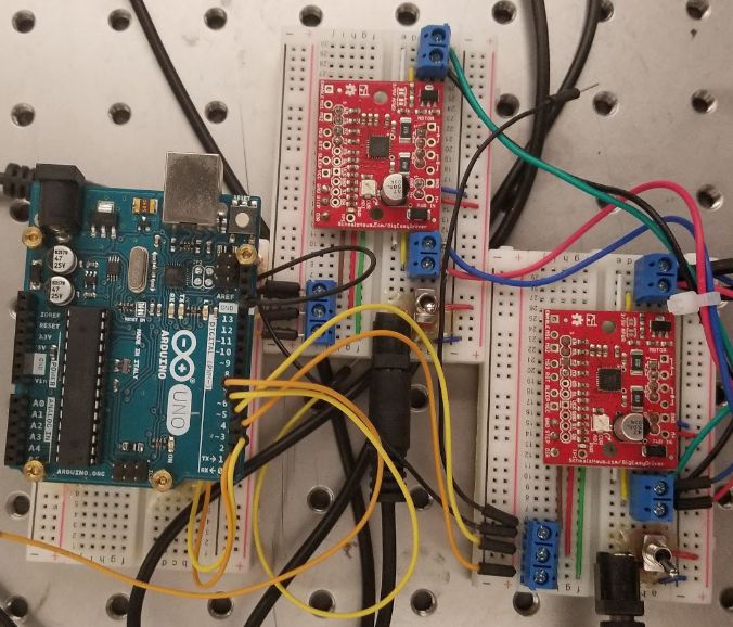
SOFT-MICROROBOTICS:
THE MANIPULATION OF ALGINATE ARTIFICIAL CELLS

                                                   Approved by:

                        Dr. Min Jun Kim, Ph.D.
                        Professor of Mechanical Engineering

                        Dr. Ali Beskok, Ph.D.
                        Professor, Department Chair of
                        Mechanical Engineering

                        Dr. Yildirim Hurmuzlu, Ph.D.
                        Professor of Mechanical Engineering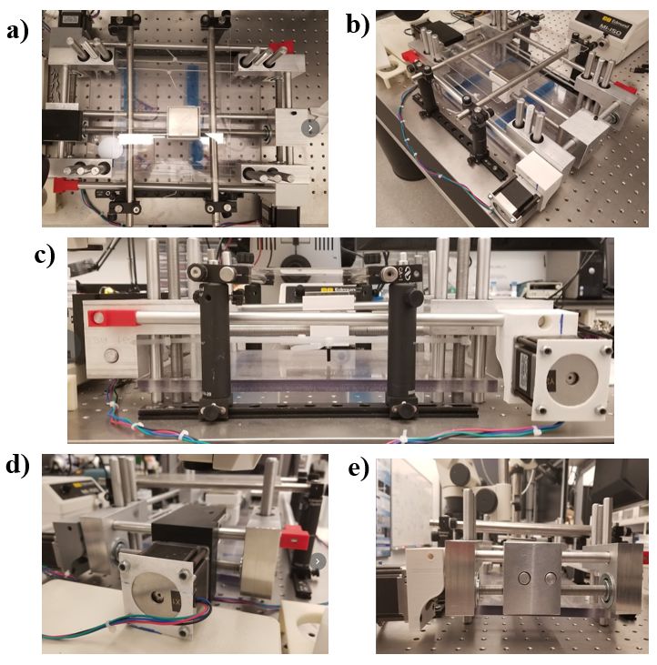
SOFT-MICROROBOTICS:

THE MANIPULATION OF ALGINATE ARTIFICIAL CELLS

  A Dissertation Presented to the Graduate Faculty of the

           Bobby B. Lyle School of Engineering

              Southern Methodist University

                            in

          Partial Fulfillment of the Requirements

                     for the degree of

        Master of Science, Mechanical Engineering

                          with a

             Major in Mechanical Engineering

                            by

                  Samuel Ian Sheckman

      B.S., Mechanical Engineering, Drexel University

                      May 19, 2018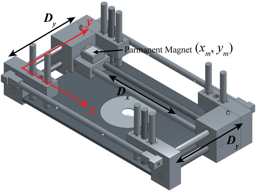
Copyright (2018)

Samuel Ian Sheckman

All Rights Reserved

         iii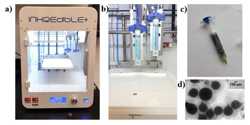
ACKNOWLEDGMENTS

   This work was supported by the National Science Foundation (IIS 1734732, IIS 1712088,
IIS 1619278), National Research Foundation of Korea and National Science Foundation
Collaboration (OISE 1713803), Korea Evaluation Institute of Industrial Technology (KEIT)
funded by the Ministry of Trade, Industry, and Energy (MOTIE)(NO. 10052980) and Open
Innovation Program of NNFC (COI1710M001). Firstly, I want to thank my advisor Dr. Min
Jun Kim for his guidance and tutelage over the course of my Undergraduate and Masters
research at Drexel University and SMU, respectively. I would like to thank my BAST LAB
colleagues Dr. Hoyeon Kim, Dr. Jamel Ali, Dr. U Kei Cheang, Louis W. Rogowski and Xiao
Zhang for lending their knowledge and encouragement to complete this work. For supporting
me for the NSF-NRF East Asia and Pacific Summer Institutes (EAPSI) Research Fellowship
(OISE 1713803), I would like to thank Dr. Chi Won Ahn and the NNFC in Daejeon, South
Korea. Additionally, I want to thank my collaborators at The University of Houston, Dr.
Aaron Becker and Sheryl Manzoor for working with me over the course of time in the BAST
Lab. To my Masters Committee, Dr. Ali Beskok and Dr. Yildirim Hurmuzlu, I want to
thank you for taking the time to assess my work.

                                           iii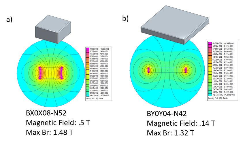
Sheckman, Samuel Ian                         B.S., Mechanical Engineering, Drexel University

Soft-Microrobotics:
The Manipulation of Alginate Artificial Cells

    Advisor: Dr. Min Jun Kim, Ph.D.
Master of Science, Mechanical Engineering degree conferred May 19, 2018
Dissertation completed April 13, 2018

    In this work, the approach to the manipulation of alginate artificial cell soft-microrobots,
both individually and in swarms is shown. Fabrication of these artificial cells were completed
through centrifugation, producing large volumes of artificial cells, encapsulated with super-
paramagnetic iron oxide nanoparticles; these artificial cells can be then externally stimulated
by an applied magnetic field. The construction of a Permeant Magnet Stage (PMS) was
produced to manipulate the artificial cells individually and in swarms. The stage function-
alizes the permanent magnet in the 2D xy-plane. Once the PMS was completed, Parallel
self-assembly (Object Particle Computation) using swarms of artificial cells in complex envi-
ronments, controlled not by individual navigation, but by a global, external magnetic force
with the same effect on each artificial cell to produce miroassemblies. A 2D grid world fac-
tory, in which all obstacles and particles are unit squares, and for each actuation, artificial
cells move maximally until they collide with an obstacle or another artificial cell. Based on
the design of an arbitrary 2D structure, this 2D grid world layout, will produce continuous
microassemblies.

                                              iv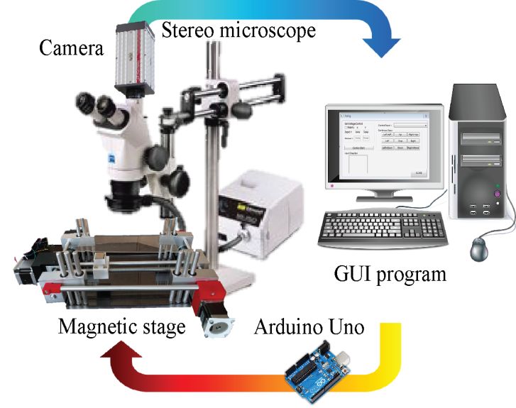
TABLE OF CONTENTS

 LIST OF FIGURES . . . . . . . . . . . . . . . . . . . . . . . . . . . . . . . . . . . . . . . . . . . . . . . . . . . . . . . . . . . . . . . .     vi

CHAPTER

  1.     INTRODUCTION . . . . . . . . . . . . . . . . . . . . . . . . . . . . . . . . . . . . . . . . . . . . . . . . . . . . . . . . . . . .          1

  2.     MATERIALS AND METHODS . . . . . . . . . . . . . . . . . . . . . . . . . . . . . . . . . . . . . . . . . . . . . . .                           6

         2.1. Alginate Artifical Cell Preparation . . . . . . . . . . . . . . . . . . . . . . . . . . . . . . . . . . . . . . . .                      6

         2.2. Pressure Driven Fabrication Method . . . . . . . . . . . . . . . . . . . . . . . . . . . . . . . . . . . . . .                           6

         2.3. Centrifugal Fabrication Method. . . . . . . . . . . . . . . . . . . . . . . . . . . . . . . . . . . . . . . . . . .                      8

         2.4. Permanent Magnet Stage (PMS) Design . . . . . . . . . . . . . . . . . . . . . . . . . . . . . . . . . . 10

         2.5. Permanent Magnet Stage (PMS) Governing Forces . . . . . . . . . . . . . . . . . . . . . . . . 13

         2.6. Object Particle Computation . . . . . . . . . . . . . . . . . . . . . . . . . . . . . . . . . . . . . . . . . . . . . 16

         2.7. Experimental setup . . . . . . . . . . . . . . . . . . . . . . . . . . . . . . . . . . . . . . . . . . . . . . . . . . . . . . 26

  3.     RESULTS AND DISCUSSION . . . . . . . . . . . . . . . . . . . . . . . . . . . . . . . . . . . . . . . . . . . . . . . . 29

         3.1. Single Motion Manipulation . . . . . . . . . . . . . . . . . . . . . . . . . . . . . . . . . . . . . . . . . . . . . . 29

         3.2. Swarm Motion Manipulation . . . . . . . . . . . . . . . . . . . . . . . . . . . . . . . . . . . . . . . . . . . . . 30

         3.3. Object Particle Computation . . . . . . . . . . . . . . . . . . . . . . . . . . . . . . . . . . . . . . . . . . . . . 33

  4.     DISCUSSION AND FUTURE WORK . . . . . . . . . . . . . . . . . . . . . . . . . . . . . . . . . . . . . . . . . 36

         4.1. Discussion . . . . . . . . . . . . . . . . . . . . . . . . . . . . . . . . . . . . . . . . . . . . . . . . . . . . . . . . . . . . . . . 36

         4.2. Future Work . . . . . . . . . . . . . . . . . . . . . . . . . . . . . . . . . . . . . . . . . . . . . . . . . . . . . . . . . . . . . 36

APPENDIX

  A. Published Works . . . . . . . . . . . . . . . . . . . . . . . . . . . . . . . . . . . . . . . . . . . . . . . . . . . . . . . . . . . . . . 38

BIBLIOGRAPHY . . . . . . . . . . . . . . . . . . . . . . . . . . . . . . . . . . . . . . . . . . . . . . . . . . . . . . . . . . . . . . . . . . . 40

                                                                          v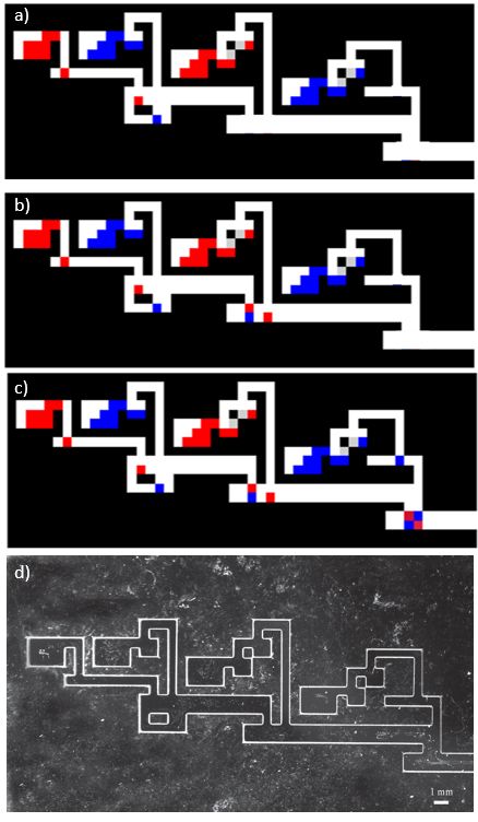
LIST OF FIGURES

Figure                                                                                                                                           Page

2.1      Pipette Pressue Driven Alginate Fabrication Method . . . . . . . . . . . . . . . . . . . . . . . . . .                                         7

2.2      Cellink Inkcredible 3D-BioPrinter . . . . . . . . . . . . . . . . . . . . . . . . . . . . . . . . . . . . . . . . . . . .                      8

2.3      Alginate Artifical Cell . . . . . . . . . . . . . . . . . . . . . . . . . . . . . . . . . . . . . . . . . . . . . . . . . . . . . . . .        9

2.4      CAD Model of PMS . . . . . . . . . . . . . . . . . . . . . . . . . . . . . . . . . . . . . . . . . . . . . . . . . . . . . . . . . 11

2.5      Final Assembly of the PMS . . . . . . . . . . . . . . . . . . . . . . . . . . . . . . . . . . . . . . . . . . . . . . . . . . 12

2.6      Ardunio Controller . . . . . . . . . . . . . . . . . . . . . . . . . . . . . . . . . . . . . . . . . . . . . . . . . . . . . . . . . . . 13

2.7      FEMM analysis of Permanent Magnets . . . . . . . . . . . . . . . . . . . . . . . . . . . . . . . . . . . . . . . 15

2.8      Polyomino Parts . . . . . . . . . . . . . . . . . . . . . . . . . . . . . . . . . . . . . . . . . . . . . . . . . . . . . . . . . . . . . 18

2.9      Algorithm 1. . . . . . . . . . . . . . . . . . . . . . . . . . . . . . . . . . . . . . . . . . . . . . . . . . . . . . . . . . . . . . . . . . 19

2.10     Algorithm 2. . . . . . . . . . . . . . . . . . . . . . . . . . . . . . . . . . . . . . . . . . . . . . . . . . . . . . . . . . . . . . . . . . 20

2.11     Algorithm 3. . . . . . . . . . . . . . . . . . . . . . . . . . . . . . . . . . . . . . . . . . . . . . . . . . . . . . . . . . . . . . . . . . 21

2.12     Deconstruction order matters if loops are present, and Hopper with five
            delays figures. . . . . . . . . . . . . . . . . . . . . . . . . . . . . . . . . . . . . . . . . . . . . . . . . . . . . . . . . . . . . 22

2.13     Algorithm 4. . . . . . . . . . . . . . . . . . . . . . . . . . . . . . . . . . . . . . . . . . . . . . . . . . . . . . . . . . . . . . . . . . 23

2.14     Algorithm 5. . . . . . . . . . . . . . . . . . . . . . . . . . . . . . . . . . . . . . . . . . . . . . . . . . . . . . . . . . . . . . . . . . 24

2.15     Worst-case cycle distance plotted as a function of polyomino size n, and
            factory size grows quadratically with the number of tiles plots. . . . . . . . . . . . . . 26

2.16     4 Polyomino Square Algorithm . . . . . . . . . . . . . . . . . . . . . . . . . . . . . . . . . . . . . . . . . . . . . . . 27

2.17     Experimental Setup . . . . . . . . . . . . . . . . . . . . . . . . . . . . . . . . . . . . . . . . . . . . . . . . . . . . . . . . . . 28

3.1      Single Artifical Cell SMU Manipulation. . . . . . . . . . . . . . . . . . . . . . . . . . . . . . . . . . . . . . . 30

3.2      Aggregation of Artifical Cell Swarm . . . . . . . . . . . . . . . . . . . . . . . . . . . . . . . . . . . . . . . . . . 31

3.3      Translational Manipulation of Artifical Cell Swarm Motion . . . . . . . . . . . . . . . . . . . . 32

                                                                         vi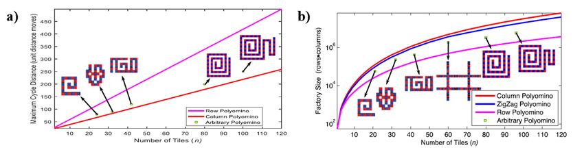
3.4   Transportation Task of Artifical Cell Swarm Motion . . . . . . . . . . . . . . . . . . . . . . . . . . 33

3.5   Object Particle Computation ALG.4. . . . . . . . . . . . . . . . . . . . . . . . . . . . . . . . . . . . . . . . . . 35

                                                          vii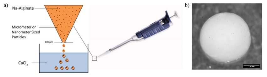
This is dedicated to my family.
Chapter 1

                                      INTRODUCTION

   Microrobotics is a growing and advancing concentration in the field of robotics and en-
gineering. As the interdisciplinary nature of the research allows an interaction between
mechanical, electrical and materials engineering with medicine and outward research fields,
the concentration is on the vanguard of science. Within the robotics research field, there is
the discipline of soft-robotics, naturally derived materials are used to mimic natural design
and create a robot to be used in situations where rigid mechanical structures would not be
capable [25, 54].

   Microrobotics has also been introduced to this new soft-material mechanism to perform
specific tasks. As such, microrobotics can be characterized as three forms of robots with
rigid-particles, soft-particles, and biological hybrids. Work over the past few decades have
shown that these particle microrobots can be manufactured with large populations (103 -1014 )
of small scale (10−9 -10−6 m) robots using diverse array of materials and techniques [14,32,38].
Since these microrobots are so small, they are ideal for several invasive medical procedures;
such as, but not limited to: minimally invasive surgery, targeted therapy, disease diagnosis,
single-cell manipulation and tissue engineering [1, 7, 48, 57, 58]. These microrobots are wire-
less controlled through external stimulis [12, 15, 17, 18, 21, 32, 55], and have been shown to
complete specific tasks [28]. Since microrobots are on the micro-scale this provides a unique
challenge to control; as limits in fabrication do not allow for or have little-to-no onboard
computing or communication ability [12, 14, 18]. These limitations make controlling swarms
of these robots individually impractical. Thus, these robotic systems are often controlled by
a global external signal (e.g. chemical gradients, electric and magnetic fields), which makes
motion planning for large robotic populations in tortuous environments difficult. Having

                                               1
only one global signal that simultaneously affects all robots at once limits the swarms ability
to perform complex operations. Independent control is possible by designing heterogeneous
particles that respond differently to the global input, but this approach requires precise
differences in each robot and is best suited for small populations. Alternatively, control
symmetry can be broken using interactions between the robot swarm and obstacles in the
environment [4, 5].
Naturally derived polysaccharide based hydrogels have presented themselves as the ideal
soft-microrobot. Their biocompatibility, hydrophilicity, as well as the ability to reversibly
encapsulate organic and inorganic materials has shown the capability of the material. Once
material is encapsulated into a hydrogel, the droplets mimic the basic structure of living
cells (membrane, cytoplasm, organelles, etc.), and as such is also referred to as an artificial
cell [8, 9, 34]. Fabricated through the process of crosslinking alginate sodium when in the
presence of divalent cations, most effectively with barium and calcium. As an over exposure
to former is toxic to nearly all living cells, calcium is the preferred method of crosslink-
ing [29]. Over time the outer polymer bilayer of the artificial cell begins to become more
porous, the internal payload is naturally released and the artificial cell reaches the end of
its usefulness. As a result, coating of the outer surface can result in the polymer layer to
become more stable, prolonging the viability of the particle. These coated particles result in
higher viability in both ex vivo and in vivo environments. These outer polymer layer is also
reactive the pH of the surrounding medium, release of encapsulated materials and change in
size occurs more rapidly. Coating agents strengthen the ionic strength of the outer polymer
layer allowing the extension of the artificial cells life [30, 41–43]. Without a coated layer,
there is still great effect temperature and pH has on the shape and rigidity of artificial cells.
Under atmosphere conditions, room temperature and neutral pH, particles remain similar
size throughout experimentation [50]. Additionally, hydrogels capibilies of encapulation en-
ables the facilitation to fabricate biosensing soft-microrobots for biomedical purposes [53].
2Single bead particles on the microscale are typically reserved for boundary surface motion
applications. The motions are characterized into two subsets, rolling motion and transla-
tional (dragging) motion, depending on the external stimulation that is experienced by the
particle. Purcells Scallop Theorem states that a reciprocating motion, such as a scallop
opening and closing its simple hinged shell, would not be sufficient to create migration at
low Reynolds number [35]. As such, a single symmetric magnetic bead, far from boundaries,
under a rotating externally applied magnetic field, will stay in the same location. A multi-
bead structure, of at least three particles, breaks the symmetry and due to its achirality
can move with a swimming motion through the media under a rotating magnetic field [10].
Thus, a single symmetric particle structure is typically manipulated using either a statically
applied magnetic field or magnetic gradient in Newtonian conditions [37]. Alginate hydrogels
has been shown to both encapsulate and ionically bond flagellar bodies. The flagella bonded
to the surface, produce a nonreciprocating motion while swimming through a medium at low
Reynolds number, are then manipulated for the purpose of locomotion of the microrobot [33].
To control the manipulation of these artificial cells, the design and fabrication of an alter-
native magnetic stimulation was sought to increase working area with decrease cost factors.
As mentioned prior, typical actuation of single particles are broken in two subsets, these
motions require external magnetic stimuli for these moving motions can be controlled using
an external rotating magnetic field from a Helmholtz coil system or a magnetic gradient by
a Maxwell coil system [2,11,32]. These coil systems are expensive and cumbersome to set up
as the power supplies can cost tens of thousands of dollars. These systems are limited by the
current the power supplies can generate and the heating effect of the working area that is
caused due by the heating of the copper wires. Producing a system that can produce an ex-
ternally applied magnetic field and have an enlarged working area introduced the concept of
a Permanent Magnet Stage. Instead of a high-power system, a permanent magnetic would be
used to drag the microrobots and alginate artificial cells to their desired destinations. This
system is designed to have interchangeable magnetics as to allow different magnetic field
3types and strengths to be used for specific applications. Research groups have conducted
similar research into permanent magnetic manipulation to maneuver particles [24,39]. These
systems are much more elaborate and would require more setup and cost. With this system,
a single global input can control the microrobotic artificial cells. The ability to manipulate
a single particle and a swarm of particles is therefore possible under these conditions.
To further the application of microrobotics, a long-sought foundation towards the cre-
ation of complex microassemblies has been needed. With the introduction of object particle
computation, multiple microrobots can be manipulated in unison by a single external input
and directed to different locations [4, 5]. Typical fabrication of multiple microassemblies
requires the use of continual microfabrication techniques which increases the initial costs
of fabrication. To decrease this effect, object particle computation allows for a single de-
sign to be constructed using traditional and nontraditional microfabrication techniques to
manufacture a specific design to fabricate parallel microassemblies continuously. To produce
constructions with microgels, groups have traditionally turned to non-robotic microfluidic
systems that utilize a variety of actuation methods, including mechanical, optical, dielec-
trophoretic, acoustophoretic, and thermophoretic [3, 13, 16, 47, 56]. While each of these
methods has proven to be capable of manipulating biological cells, each method has sig-
nificant drawbacks that limit their widespread application. For example, microscale me-
chanical, acoustophoretic, and thermophoretic manipulation methods use stimuli that can
be potentially lethal to live cells [23]. Furthermore, most, if not all, of these techniques re-
quire expensive equipment and lack control schemes necessary to precisely manipulate large
numbers of cells autonomously [45,51,52]. Obstacles present in the workspace can determin-
istically break the symmetry of approximately identical robotic swarms, enabling positional
configuration of robots [6], while using biologically compatible magnetic stimulus. Given
sufficient free space, a single obstacle is sufficient for positional control over N particles.
This method can be used to form complex assemblies out of large swarms of mobile micro-
robotic building blocks, using only a single global input signal. This algorithm uses path
4planning techniques described in [36, 49]. Using these techniques this methodology can be
used towards the development of drug delivery and tissue engineering applications.
This manuscript follows the following outline: 1) Introduction, 2) Methods, background
in artificial cell fabrication, design and fabrication of the Permanent Magnet Stage (PMS)
Controller, theory of the object particle computation, and experimental setup, 3) Experi-
mental Results, and 4) Discussion and Future work.
5Chapter 2
MATERIALS AND METHODS
2.1. Alginate Artifical Cell Preparation
The primary microrobot during experimentation is the artifical cells produced from algi-
nate hydrogels. The formation of the hydrogel is caused by a crosslinking process between
Alginate-Na and Calcium Chloride [29]; other crosslinking agents are available, but calcium is
the only one that is not harmful to the body. The encapsulated the payload can be released
using chelating agents, most prominently ethylenediaminetetraacetic acid (EDTA). Using
solutions of Sodium Alginate interacting with Calcium Chloride, the artificial cells predomi-
nately in most experiments with the encapulsation of iron oxide paramagnetic nanoparticles.
Paramagnetic nanoparticles are encapsulated to allow for steerable propulsion.
2.2. Pressure Driven Fabrication Method
To fabricate alginate artificial cells on the macro-scale, a purely pressure driven method
of manufacturing is deployed. Typically, the use of a pipette is typical for this type of fabri-
cation, due to the ease of use and wide availability. Pipettes follow the capillary principles
of fluid mechanics and as such, the size of the particle is expressed by the Young-Laplace
equation [40]. The Young-Laplace equation is as follows:
1 1
∆P = 2σp [ − ] (2.1)
Rd Rp
6where ∆P , σp , Rd , and Rp , are the change in pressure, surface tension of the alginate so-
lution, radius of the alginate particle, and the radius of the pipette, respectively. Depending
on the change in pressure, the size of the particle will alter. Thus, the use of pipettes will
produce alginate artifical cells, but results are be scattered due to human error and input
of pressure into the pipette tip. This method can produce large scale millimeter alginate
artificial cells, when large scale as shown in figure 2.1 below. Figure 2.1 shows the pipette
process as well as a millimeter-scale alginate microrobot.
Figure 2.1. a) Pressue Driven Pipette Process. A concentration of Alginate-Na is mixed
with superparagmanetic iron oxide nanoparticles and in side of the pipette tip. Pressure
is then place on the pipette to produce droplets of the particles of the desired size into a
Calcium Cloride bath. Crosslinking process is instantaneous. (Image Courtesy of Dr. Jamel
Ali) b) A millimeter scale artifical cell, produced via Pressure Driven Method. Scale bar is
1mm.
Additionally, this pressure driven method can produce droplets using a Bio 3D-printer.
Due to recent advances in 3D printing and the expiring of patents in late 2000’s, the 3D
printing industry has exploded. Most recently, the biggest advancements have been in the
field of biological 3D-printers. Typically, these systems use sryinges to change resolution,
extrusion based bioprinting produced from a pnumatic valve system allows for consistant
particle droplets to be formed [44]. These however are more tear shaped to surface tension
7from the nozzle. A typical cylindrical needle gage will require approximatley 180-190 kPa
to produce a single droplet, where as use of a conical needle gage will drastically reduce the
applied pressure to approximately 10-15 kPa. Our lab currently possess a Cellink Inkredi-
ble+ 3D-BioPrinter, this system can be seen in figure 2.2.
Figure 2.2. 3D-BioPrinter Process. a) The Cellink Incredible+ with current pressue appli-
cation in the lower left corner, pressue is read in kPa. b) Duel syringe set-up displayed, the
current needle gage 20. c) A Cellink Sryinge with Alginate-Na filled and a 100µm diameter
conical needle before placed inside the Inkredible+ for droplet manufacturing. d) Alginate
Artifical Cells after fabricated through 3D-Biprinter process, scale bar is 100µm
2.3. Centrifugal Fabrication Method
The use of the centrifugal method produces Alginate artifical cells on the scale of 500µm
to 80µm, as shown through experiemental results in figure 2.3(a). To determine the size of
the final particle the following governing equation used [2], and thus explained as:
8s
3 6dn σp
dp = (2.2)
ρp g
where dn , σp , ρp , and g, are the diameter of the nozzle, surface tension of the alginate
solution, density of alginate solution, and the applied gravitational force, respectively. The
surface tension of alginate is 65.46 mN/m [20], and a density of 1.1 g/cm3 .
Figure 2.3. Alginate Artifical Cell Fabrication results. a) Average particle size after changing
concentration. b) 150µm Alginate Artifical Cell under 1500 rcf and a 27g needle [46]
To conduct the fabrication of artificial cells with this method, a microcentrifuge is used.
The change in relative centrifugal force (rcf) is the acceleration in a centrifuge normalized to
Earths gravity. This rcf value is correlated to the size of the needle diameter producing the
artificial cells. The higher the rcf being applied, the smaller the artificial cell, this is however
limited by the gage size of the needle. Large needle gages such as 25g will produce larger
particles at 1000 rcf compared to a 30g needle under the same conditions. Particle size can
be drastically decreased, this can also be seen in the change in concentration of Alginate-Na
being used in crosslinking. The higher the concentration, the smaller the overall size of the
particle under similar conditions. The consistency of the centrifugal method is its advantage
9over the pressure driven method, using equation 2.2 an alginate artificial cell of reasonable
diameter can be fabricated.
The process to produce these artificial cells is as follows: 1) Using a 1.5ml microcentrifuge
tube, punch a hole approximately the size of the diameter of the needle gage required for
fabrication in the center of the tube cap. 2) After thoroughly cleaning the microcentrifuge
tube of debris, place the desired concentration of Calcium Chloride approximately 0.1-0.2ml
below the tip of the needle. The needle must not touch the as the crosslinking of Alginate-Na
and Calcium Chloride is nearly instantaneous reaction once there is contact. 3) Enter the
desired concentration of Alginate-Na in the cap of the needle. Finally, 4) Place the micro-
centrifuge tube into a microcentrifuge with counter weight and enter the desired rcf. These
steps result in the mass fabrication of alginate artificial cells, with the encapsulation of a
stimulating material such as iron oxide, controllability is achievable when placed under an
externally applied magnetic field.
The average particle size during experimentation is approximately 300 µm, and were com-
posed of a concentration of 5 percent (w/v) Alginate-Na and 5 percent (w/v) concentration
of CaCl2 , and then encapsulated with 10 percent (w/v) superparamagnetic nanoparticles
(Iron oxide, Sigma-Aldrich). Using a 27g needle and 300 rcf.
2.4. Permanent Magnet Stage (PMS) Design
The proposed permanent magnet stage controller would allow for interchangeable perma-
nent magnets. This parameter of design became of utmost importance, as different applica-
tion would require a different magnetic field. Depending on the size of the magnet field, the
Field of play needs to be large enough so when the magnet is not being used, it would not
interfere with any microrobot shown in the field of view. Field of play, as we have termed it,
describes the total accolated space the magnet can move in the xy-plane. The total space
10in the field of play, is 12 x 24 cm2 . The field of view, displayed through a microscope allows
for movement to viewed and physically analyzed. Typically, the field of view is in the center
of the field of play, which allows for the magnet to safely exit any time the magnetic field is
needed on the environment.
An additional parameter of the design was that the stage must work on an inverted mi-
croscope and a stereoscopic microscope. This would allow for a smaller and smaller field
of view and smaller microrobots to be investigated; as inverted microscopes allow for in-
terchangeable optics to be used, generating greater magnification than that of traditional
stereoscopic microscopes. As such, there were some imitations to the size of the stage. Using
a Olympus IX50 inverted microscope as the basis for the stage dimensions, the overall length
of the stage comes to be 22.86 x 35.56 cm2 . The height of the stage is 15.24 cm, from the
base of to the top of the z -axis. The figure below shows the CAD model of the stage, as it
would be used under a stereoscopic microscope.
Figure 2.4. CAD Model of PMS [46]
Raw material for the stage was 6061 T-6 Aluminum (McMaster-Carr, Atlanta Ga, USA).
The base is a 1.27 cm thick polycarbonate sheet. Stepper motor holders were designed in
11CAD and printed by using 3D printer. A seperate adjustable stage, from Edmund Optics,
is used to reduce vibration from the movement of the permanent magnet.
Figure 2.5. Final Assembly of the PMS. a) Top View. b) Isometric View. c) Front View.
d) Left View. e) Right View.
Using an Ardunio R3, two BigEasy Stepper Motor Drivers, and three stepper motors
(Sparkfun.com); the stage was controlled through a designed graphic user interface (GUI)
by way of a C++ program. Using programmed C++, it allows giving the control input
signal to the Ardunio R3 by USB communication during the sampling time of 0.5 s. Then,
the Ardunio R3 generates the digital signal to BigEay Stepper Motor Drivers in terms of
the direction and the turn of steps. Stepper Motor Drivers controls the stepper Motors to
12follow the desired input rotation with a maximum acceleration.
Figure 2.6. Ardunio Controller. Two BigEasy Stepper Motor Drivers are used and connected
through breadboards to the stepper motors.
Each input was manually entered into the C++ based GUI, then, the magnetic would
move as a continuous function, or in single steps. The time step of the movement was
shortened to very small value to allow the magnetic particles to move across the field of
view. If the magnet moved to quickly, the particles would not react to magnetic field. A bal-
ance between speed and strength of the magnet needed to be found in this open-loop system.
2.5. Permanent Magnet Stage (PMS) Governing Forces
Governing the controlling system is the permanent magnet, distributing the magnetic
field upon which the microrobots are being manipulated. As described in [19, 31], using the
equation for magnetic flux density of a permanent magnet can be found as:
13B = µ0 (H + M) (2.3)
where, µ0 , H and M are the permeability of free space, the magnetic field and the magnetiza-
tion produced by the permanent magnet, respectively. The value for µ0 is 1.256x10⁻⁶ H/m.
Further analysis can be performed to find the magnetic force being exerted by the permanent
magnet and displayed on the magnetic dipole moment m.
Fm = ∇(U ) = ∇(m · B) = (∇m) · B + m · B = (m · ∇)B (2.4)
where U represents the gradient of the magnetic dipole energy. Since the alginate micro-
robots encapsulate paramagnetic nanoparticles and the microrobots are in a non-magnetic
fluid, therefore m = V M = V H. From equations (2.3) and (2.4), as well knowing the rela-
tionship of (1+χ) as the relative permeability of the media, represented by µr ; the force can
be rewritten as:
Vχ
Fm = (B · ∇)B (2.5)
µ0 µr
where V and χ is the volume of an alginate microrobot and the effective magnetic suscep-
tibility, respectively. The fluid medium in experiments is a solution of Deionized water and
tween 20, this solution is shows no magnetic properties. Thus, the effective susceptibility of
the medium is assumed to be 1.
The magnet used in the experiments was a NdFeB, Grade N42/N52 (KJ Magnetics,
Pipersville PA, USA). For the N42 magnet, the size was 5.08 x 5.08 cm2 , with a thickness of
0.635 cm. The N52 magnet size was 2.54 x 2.54 cm2 , with a thickness of 1.27 cm. For design
14a large magnet was used to determine space, the N52 was used more in experimentation.
The FEMM analysis of both magnets are shown below in figure 2.7.
Figure 2.7. FEMM analysis of Permanent Magnets. a) N52 NdFeB magnet b) N42 NdFeB
magent.
These are not the only forces governing the microrobots, drag forces to be considered.
At the small scale, forces such as gravity can be neglected and forces viscous forces become
more of an obstacle to overcome. For this reason, the drag the microrobots are experiencing
needs to be calculated in the total force equation. The drag force of a microrobot at low
Reynolds Number [22], can be written as:
Fd = 6πµvR (2.6)
15where V , R, and µ are defined as the velocity, radius of the microrobot, and the viscosity
of the fluid, respectively. Since the fluid is remaining still in our case, the velocity is that
experience by the microrobot. When combining Eq. (2.5) and Eq. (2.6), the equation for
the total force experienced by a microrobot to be:
Vχ
Fm = (B · ∇)B − 6πµvR (2.7)
µ0 µr
2.6. Object Particle Computation
Through the use of obstacle laden environment, where artificial cells or microrobots, move
through a maze like structure to reach a final destination. In this algorithmic procedure,
alginate artifical cells are hereby termed polyominoes, to describe the arbitary 2D geometric
figure by the joining one or more equal ’squares’ edge to edge [27]. The maze is designed to
interact with the particles to create pre-determined complexes at the end result. A swarm
of microrobots are controlled using a global input and move until an obstacle stopped them
from moving any further. Particle computation uses logic gates and wiring gates to move
and connect the microrobots from stage one to final assembly [5]. From rules of object par-
ticle computation, an obstacle laden environment can be determined and a Model can be
expressed as [4, 5]:
1. A 2D workspace is filled with a number of unit-square particle and some fixed unit-
square blocks. Each unit square in the works space is either free, which a robot can occupy
or obstacle which a particle may not occupy.
2. All particles are commanded in unison: the valid commands are Go Up (u), Go Right
(r), Go Down (d), Go Left (l).
163. The particles all move in the commanded direction until the hit an obstacle or a
stationary robot.
The polyominoes will continue to move in the commands given, until the final assembly
is created. Further development of these laws to produce individual factories to manufacture
parallel microassemblies of nearly any shape desired is expressed in Manzoor et al. [27], and
shown here in this section. These algorithms described in this section were developed at
The University of Houston in collaboration with Dr. Aaron Becker and Sheryl Manzoor, the
matlab code of these algorithms can be found at [26].
Arbitary 2D Shapes Require Two Particle Species
Polyominoes have four-point connectivity: a 4-connected square is a neighbor to every
square that shares an edge with it.
Lemma 1: Any polyomino can be constructed using just two species
Proof: Label a gridwith an alternating pattern like a checkerboard. Any desired poly-
omino can be constructed on this checkerboard, and all joints are between dissimilar species.
An example shape is shown in Fig. 2.8. Red and blue colors are used to indicate particles
of different species.
The sufficiency of two species to construct any shape gives many options for implementa-
tion. The two species could correspond to any gendered connection, including ionic charge,
magnetic polarity, or hook-and-loop type fasteners. Large populations of these two species
can then be stored in separate hoppers and, like two-part epoxy, only assemble when dis-
similar particles come in contact.
17Figure 2.8. Polyomino Parts. Assembly difficulty increases from left to right [27].
Complexity Handled in This Paper
2D part geometries vary in difficulty. Fig. 2.8 shows parts with increasing complexity.
Label the first particle in the assembly process the seed particle. Part 1 is shaped as a
# symbol. Though it has an interior hole, any of the 16 particles could serve as the seed
particle, and the shape could be constructed around it. The second shape is a spiral, and
must be constructed from the inside-out. If the outer spiral was completed first, there would
be no path to add particles to finish the interior because added particles would have to slide
past compatible particles. Increasing the number of species would not solve this problem,
because there is a narrow passage through the spiral that forces incoming parts to slide past
the edges of all the bonded particles. The third shape contains a loop, and the interior must
be finished before the loop is closed. Shape 4 is the combination of a left-handed and a
right-handed spiral. Adding one particle at a time in 2D cannot assemble this part, because
each spiral must be constructed from the inside-out. Instead, this part must be divided into
subassemblies that are each constructed, and then combined. Shape 5 contains compound
overhangs, and may be impossible to construct with additive 2D manufacturing using only
two species. The algorithms in this letter detect if the desired shape can be constructed one
particle at a time. If so, a build order is provided, and a factory layout is designed.
Discovering a Build Path
18Given a polyomino, Alg. 1 determines if the polyomino can be built by adding one com-
ponent at a time. The problem of determining a build order is difficult because there are O(
n!) possible build orders, and many of them may violate the constraints shown in the rules
established previously. Each new tile must have a straight-line path to its goal position in
the polyomino that does not collide with any other tile, does not slide past an opposite specie
tile, and terminates in a mating configuration with an opposite specie tile. However, as in
many robotics problems, the inverse problem of deconstruction is easier than the forward
problem of construction.
Figure 2.9. Algorithm 1: Finding the Build Path [27].
Alg. 1 first assigns each tile in the polyomino a color, then calls the recursive function
DECOMPOSE, which returns either a build order of polyomino coordinates and the direc-
tions to build, or an empty list if the part cannot be constructed. DECOMPOSE starts
by calling the function ERODE. ERODE first counts the number of components in the 8-
connected freespace. An 8-connected square is a neighbor to every square that shares an
edge or vertex with it. If there is more than one connected component, the polyomino con-
tains loops. ERODE maintains an array of the remaining tiles in the polyomino R. In the
inner for loop at line 2, a temporary array T is generated that contains all but the j th tile
in R sorted by the number of neighbors so a tile with one neighbor is checked before tiles
with two or three. This for loop simply checks (1) if the j th tile can be removed along a
straight-line path without colliding with any other particle or sliding past an opposite specie
19tile in line 2, (2) that its removal does not fragment the remaining polyomino into more
than one piece in line 2, and (3) that its removal does not break a loop in line 2. If no
loops are present, this algorithm requires at most n/2(1 + n) iterations, because there are n
particles to remove, and each iteration considers one less particle than the previous iteration.
Figure 2.10. Algorithm 2: ERODE [27].
Polyominoes with loops require care, because decomposing them in the wrong order can
make disassembly impossible, as shown in 2.12a. If loops exist then ERODE may return
only a partial decomposition, so DECOMPOSE must then try every possible break point
and recursively call DECOMPOSE until either a solution is found, or all possible decomposi-
tion orders have been tested. The worst-case number of function calls of DECOMPOSE are
proportional to the factorial of the number of loops, O (|8-CONNCOMP(¬ P)|!). Though
20large, this is much less than O( n!).
Figure 2.11. Algorithm 3: DECOMPOSE [27].
Hopper Construction
Two-part adhesives react when components mix. Placing components in separate con-
tainers prevents mixing. Similarly, storing many particles of a single species in separate
containers allows controlled mixing. We can design part hoppers, containers that store simi-
larly labelled particles. These particles will not bond with each other. The hopper shown in
2.12b releases one particle every cycle. Delay blocks are used to ensure the nth part hopper
does not start releasing particles until cycle n. For ease of exposition, this letter has a unique
hopper for each tile position. This enables precise positioning of different materials, but a
particle logic system could use just two hoppers, similar to our particle logic systems in [5].
Part Assembly Jigs
21Figure 2.12. a) Deconstruction order matters if loops are present. Loops occur when the
8-connected freespace has more than one connected component. In the top row the green
tile is removed first, resulting in a polyomino that cannot be decomposed. However, if the
bottom right tile is removed first, deconstruction is possible. b) Hopper with five delays.
The hopper is filled with similarly-labelled robots that will not combine. Every clockwise
command cycle releases one robot from the hopper. [27]
22Assembly is an iterative procedure. A factory layout is generated by BUILDFAC-
TORY(P,nc ), described in Alg. 4. This function takes a 2D polyomino P and, if P has
a valid build path, designs an obstacle layout to generate nc copies of the polyomino. A
polyomino is composed of |P| = n tiles. For each tile, the function FACTORYADDTILE (nc
, b,m,C,c,w) described in Alg. 5 is called to generate an obstacle configuration A. A forms
a hopper that releases a particle each iteration and a chamber that temporarily holds the
partially assembled polyomino b and guides the new particle C to the correct mating position.
Figure 2.13. Algorithm 4: Finding the Build Path [27].
Analysis
Once the algorithms have been processes for specific polyomino buildfactory, these al-
gorithms need to be analyzed to give approximate simulations. These are processed by
calculating the Maximum Distance Travelled and the Space Required, the end result is a
simulation of a buildfactory.
Maximum Distance Travelled
23Figure 2.14. Algorithm 5: Factory Add Tile [27].
Running a factory simulation has three phases: ramp up, production, and wind down.
During the n−1 ramp up cycles, the first polyomino is being constructed one tile at a time
and no polyominoes are produced. Clever design of delays in the part hoppers ensures no
unconnected tiles are released. During production cycles, one polyomino is finished each cy-
cle. Once the first part hopper empties, the n−1 wind down cycles each produce a complete
polyomino as each successive hopper empties. This section analyzes maximum distance,
defined as the maximum distance any tile must move. There are two results, construction
distance, the maximum distance required to assemble a single polyomino from scratch, and
cycle distance, the maximum distance required during production cycles to advance all par-
tial assemblies one cycle. Since a polyomino contains n tiles, the construction distance during
production cycles is n· (cycle distance).
Cycle distance is the sum of the maximum distances moved in each direction. As shown
in figure 2.15a, polyominoes shaped as a n x 1 row require the longest distance of 4n + 16.
Polyominoes shaped as a 1 x n column requires the least distance of 2n + 16. Construction
distance therefore requires O( n2 ) distance.
24Space Required
The space required by a factory is a function of the widths of individual sub-factories
and height of the last sub-factory. The first sub-factory is constructed separately and it does
not have any delay. Beginning from the second sub-factory, height can be computed as a
function of the number of copies nc of the polyomino, width of the hopper w, position of
the sub-factory i, and rows of the sub-assembled polyomino by as in (2.8). If a tile is added
before the top row of b, then an additional row is added to the height. The width of the
sub-factory can be calculated similarly as in (2.9) and (2.10). In a case where twice of bx
is greater than widthhopper+delays then additional columns are added to the left of the sub-
factory. When a tile is added to b using a down move, width also depends on the location
of the column, columnloc , to which the tile is added.
nc i
height(i) = d e + 2(d e + by ) + {4, f or m = l or d, i ≥ 2; 7, f or m = u or r, i ≥ 2 (2.8)
w 2
i
widthhopper+delays = w + 2d e + 8, i ≥ 2 (2.9)
2
width(i) = widthhopper+delays + {bx − columnloc , f or m = d; 0, f or m 6= d (2.10)
Because a factory requires O(n) rows and O(n) columns, the total required space is
O(n2 ). As shown in figure 2.15b, the required size is upper bounded by column-shaped
25polyominoes and lower bounded by row-shaped polyominoes, and is O(n2 ).
Figure 2.15. a) Worst-case cycle distance plotted as a function of polyomino size n.The
cycle distance is the sum of distances to move during the r, d, l, u moves each cycle. Cycle
distance increases linearly with polyomino size and is upper bounded by row parts and lower
bounded by column parts. Total construction distance for a particle is n·cycle distance. b)
Factory size grows quadratically with the number of tiles. [27]
From these Algorithms, a square shape from 4 polyominoes was simulated. From this
simulation a microchannel system was then fabricated to test the validity of the algorithms
of object particle computation under parallel global inputs. The simulated system is shown
in figure 2.16(a-c), below.
On a 2in silicon wafer, this 4 Polyomino Algorithm was produced. After bringing the
design into AutoCAD, the algorithm was then fabricated into a film mask (CAD/Art Ser-
vices, Brandon OR, USA) for microfabrication purposes. The thickness of the microfludic
channels were approximately 300µm and individual channels were approximately 300µm in
width. The channel was fabricated using SU-8 2150 and used contact exposure to produce
the pattern, after development, the channel was cleaned and ready for experimentation. The
final product is shown in figure 2.16(d).
26Figure 2.16. 4 Polyomino Square Algorithm. a) Algorithm after 6 inputs have been made
into the system. b) Continued input leads to the fabrication of sub-polyomino microassembly.
c) Final polyomino microassembly is shown in the bottom right corner. (Image Courtesy of
Dr. Aaron Becker and Sheryl Manzoor). d) The microfludic channel device of a 4-polyomino
square after microfabrication thickness of channels is approximately 300µm.
272.7. Experimental setup
When completing experiments with the Permanent Magnet Stage (PMS), the experi-
mental setup described here was used. Experiments were conducted under a Zeiss Stemi
2000-C Stereoscopic Microscope. The experimental images were observed through a Motion
Pro X3 camera. All images were captured at a frame rate of 30 fps. Figure 2.17 shows the
experimental setup. From the initial inputs from the C++ program, the Arduino R3 relays
the information to the stepper motor drivers. The control inputs passed through the drivers
every 0.5 seconds. Thus, the permanent magnet moved with a velocity of 150 µm/s. The
experimental chamber was made of Polydimethylsiloxane (PDMS), a 35mm petri dish, or a
microfluidic device. The chamber was filled with a solution of Tween 20 and Deionized Water.
Figure 2.17. Experimental Setup [46]
28Chapter 3
RESULTS AND DISCUSSION
3.1. Single Motion Manipulation
Actuation of the stage controller can show that the manufactured microrobots can be
fully controllable. Initial commands began with a sequence of , the
alginate microrobots began to move as the magnet moved underneath. The initial position of
the alginate microrobot was manipulated to create a box. In this experiment, the interaction
of one singular alginate microrobot was demonstrated to show the ability to overcome the
drag force using the magnetic field of a permanent magnet. Still, overcoming the drag of the
alginate microrobot proved to be an individual challenge and required play with the control
scheme of the permanent magnet location.
The permanent magnet was initially placed in the center of the field of view. At this
point the alginate microrobot would not move. As the initial command was given the per-
manent magnet would move , as the magnet moved over the alginate microrobot,
the microrobot would not move until the trailing dipole of the magnet moved underneath.
Following the magnets trailing dipole, the alginate microrobot moves to its destination. To
allow the alginate microrobot to stop, the permanent magnet moves, in this case, to the center of the microrobot. Through manipulation, where the magnet moves through
the field of play with a velocity of 150 µm/s, a distance is created between the magnet and
alginate microrobot, as such the alginate microrobot followed the permanent magnet with
a varied mobility. In Fig. 3.1(a)-(c), a single alginate microrobot of 300 µm in diameter
was manipulated to spell SMU. Due to the limited input direction, the heading angle for the
29motion of aglginate microrobot is not varied.
Figure 3.1. Resultant trajectories of a single alginate microrobot using manual control. (a)
S trajectory during s, (b) M trajectory during 109 s, (c) U trajectory during 61 s. The scale
bar represents 1 mm [46].
3.2. Swarm Motion Manipulation
Using the suggested magnetic stage controller, it is available to move multiple alginate mi-
crorobots and they swarm as a group. In order to swarm, the randomly distributed alginate
microrobots need to be gathered as a group. The alginate microrobots in this experiment are
approximately 300 µm in diameter. In the experiment, the separately located microrobots
were illustrated in Fig. 3.2(a). Then, we located the permanent magnet at the A position
and the separately located individual microrobot were gathered around the A position as
shown in Fig. 3.2(b). The alginate microrobots were attracted by the magnetic field from
the permanent magnet.
However, the alginate microrobot had less attracted force because of the long distance from
the permanent magnet. Thus, the permanent magnet was moved to the B position in order
to put those alginate microrobots close to the magnet. As a result, the most alginate mi-
crorobots were gathered around the B position as indicated in Fig. 3.2(d). As the magnet
moved around the boundary of field, it will help gather all microrobot since the magnet can
be of a strong magnetic field area.
30Figure 3.2. Aggregation motion for swarming group of alginate microrobots. (a) Initial
distribution of each alginate microrobot at 0 s, (b) The instant motion when the permanent
magnet was located at A position during 34 s, (c) The resultant location of alginate micro-
robots when the magnet was relocated the B position after 45 s passed from (b), (d) The
final location of all microrobots after 28 s. The scale bar represents 1 mm [46].
Once the microrobots were gathered at the certain location, we made a swarm motion by
moving the magnet. In Fig. 3.3(a), the more than 100 alginate microrobots were positioned
at the left side. After the magnet moved toward the right side, they followed the magnet
movement as shown in Fig. 3.3(b). As seen in Fig. 3.3, the drag forces of the alginate
microrobots can be an issue at times. The trailing alginate microrobots of the swarm can
be seen to have moved very little from the initial location of 0 s.
Following the experiments with alginate microrobot swarms, an additional task of moving
a singular object was perused. In this experiment, the diameter size of the alginate micro-
robots are 300 µm. Using a 2.6 2.7 mm piece of PDMS, the alginate microrobots were then
manipulated to move from their initial position seen in Fig. 3.4(a), as the magnet was moved
from this position to is final position, the microrobots moved underneath of the PDMS piece.
The some microrobots were in contact with the piece as the flow moved it across the field of
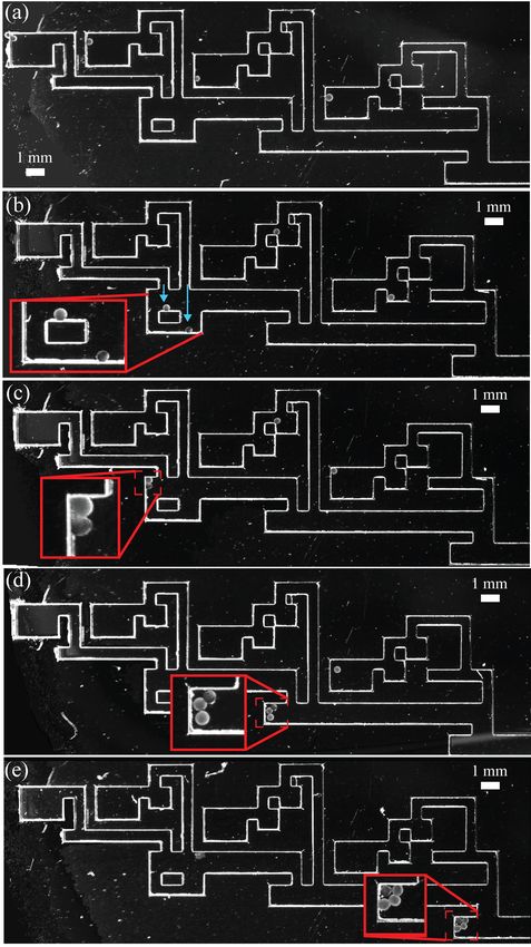
31Figure 3.3. Translational swarming motion of alginate microrobots. (a) Initial positions of
a swarming group at 0 s, The permanent magnet headed toward the right side forward the
front of alginate microrobots and the motion was shown at (b), (c), (d), and (e). The scale
bar represents 1mm [46].
32view. Figure 3.4(d) shows the final position of the piece. The total distance the PDMS piece
moved was 7.6 mm, over a 34 s span. This experiment result indicates that the swarming
alginate microrobot are available to do microscale transportation task in the low Reynolds
number.
Figure 3.4. Transport task using swarming alginate microrobots. (a) Initial positions of a
swarming group and a PDMS chunk(0 s), (b) Transport task motion at 16 s, (c) Transport
task motion at 25 s, (d) Transport task motion at 34 s. The scale bar represents 1mm [46].
333.3. Object Particle Computation
With the microfludic factory network described in previously, undetermed, alginate mi-
crorobots were transported at each hopper, by way of a pipette. To show the process, one
alginate particle was loaded in each hopper. The experimental channel was placed at the
center of the stage. The magnet centered beneath the microfluidic factory layout. This po-
sition was saved as the home position for the permanent magnet. Stepper motors controlled
the stage position. An Arduino UNO programmed in C++ commanded these step-per mo-
tors using a 2 Hz control loop. After a command was initiated, such as each direction in
the sequence, the permanent magnet was returned to the home position to
better control the distribution of the magnetic gradient. The layout was observed through
a stereomicroscope and the installed camera (Motion Pro X3) captured the procedure at 30
fps. Using 0.65x magnification in the stereomicroscope, the observed field of view is 23.6 x
18.9 mm2 .
Using a factory layout generated by a 4-polyomino square, we demonstrated micro-scale
assembly using multiple alginate microrobots, the average microrobot diameter was 300 µm.
4-polyonimo square algorithm is shown in figure 3.5(a), the system shows the completion of
square polyominoes. The initial scene in the microscale is shown in Fig. 3.5(a). The first
assembly operation was then orchestrated by moving the magnet in a clockwise direction,
following the sequence as indicated in Fig. 3.5(b-d). Each input was applied
sufficiently long to ensure all alginate microrobots touched a wall. Completion of the poly-
omino is shown in Fig. 3.5(e).
34Figure 3.5. Showing the experimental results of ALG 4. (a) shows the individual alginate in
its initial position. (b) After initial movements of the , the alginate microrobots
move to the position shown. (c) After inputs are put into the system to produce the
first multi-microrobot polyomino. (d) Shows the next three microrobot polyomino after ap-
plying multiple sequences. (e) After the alginate microrobots have moved through
the microfluidic factory layout, final product of the 4 polyomino algorithm is shown [27].
35Chapter 4
DISCUSSION AND FUTURE WORK
4.1. Discussion
This work has shown the successful manipulation of single and swarms of alginate arti-
ficial cell soft-microrobots while using the permanent magnet stage. Individual and swarm
manipulation showed the capacities to conduct specific tasks. Single microrobots were made
to spell out SMU, disperesed particles were shown to aggregate and move sufficiently in
swarms. The swarms were then made to move left to right and remained in a grouping
throughout actuation with some breaking away from the cluster. Additionally, the task to
move a single piece was PDMS was completed successfully. The successful 4 square poly-
omino microassembly was completed using the permanent magnet stage, this was done by
moving the the permanent magnet in a clockwise direction and moving in the motion as described in the rules of object particle computation for parallel assemblies.
4.2. Future Work
Further development is needed in the robustness of the microfluidic environment for the
object particle computation. Investigation into this process has begun and a new microflu-
idic system has been fabricated with a rail system, as to reduce surface friction direction on
the one contact point and help assist the particle as it moves through the system. Work
in improving the PMS for autonomous control is also being investigated, as well as adding
an additional motor specifically to rotate the permanent magnet. Rotation of the perma-
nent magnet will allow the PMS to have rolling motion manipulation as well as dragging
36manipulation. Additionally, development of artificial cell biosensing capabilities, such as
the encapsulation of gold nanorods to sense the change in temperature and cause controlled
deformations in the particle.
37Appendix A
Published Works
Journal Papers
Manzoor, S., Sheckman, S., Lonsford, J., Kim, H., Kim, M.J., Becker, A.
Parallel Self-Assembly of Polyominoes under Uniform Control Inputs
IEEE Robotics and Automation Letters, 2017.
Ali, J., Cheang, U., Liu, Y., Kim, H., Rogowski, L., Sheckman, S., Patel, P., Sun, W., Kim,
M.J.
Fabrication and Magnetic Control of Alginate-based Soft-microrobots
APL, 2016.
Conference Papers
Zhang, X., Kim, H., Rogowski, L., Sheckman, S., Kim, M.J.
Development and Implementation of 3D hexapole magnetic tweezer system for
micromanipulations
The IEEE International Conference on Robotics and Automation (ICRA), 2018
Manzoor, S., Sheckman, S., Lonsford, J., Kim, H., Kim, M.J., Becker, A.
Parallel Self-Assembly of Polyominoes under Uniform Control Inputs
IEEE/RSJ International Conference on Intelligent Robots and Systems (IROS), 2017.
Sheckman, S., Kim, H. Manzoor, S., Rogowski, L., Huang, L., Zhang, X., Becker, A., Kim,
M.J.
Manipulation and Control of Microrobots Using A Novel Permanent Magnet Stage
KROS Conference of Ubiquitous Robots and Ambient Intelligence (URAI), 2017
Sheckman, S., Kim, H. Manzoor, S., Rogowski, L., Huang, L., Zhang, X., Leclerc, J.,
Becker, A., Kim, M.J.
38Manipulation of Alginate Microrobots by Permanent Magnet Stage
IEEE Manipulation, Automation and Robotics at Small Scales (MARSS), 2017.
Zhang, X., Kim, H., Rogowski, L., Sheckman, S., Kim, M.J.
Novel 3D Magnetic Tweezer System for Microswimmer Manipulations
KROS Conference of Ubiquitous Robots and Ambient Intelligence (URAI), 2017
Rogowski, L., Zhang, X., Kim, H., Sheckman, S., Kim, D., Kim, M.J.
Swimming in Synthetic Muscin
KROS Conference of Ubiquitous Robots and Ambient Intelligence (URAI), 2017
39You can also read