MinoanER: Schema-Agnostic, Non-Iterative, Massively Parallel Resolution of Web Entities
←
→
Page content transcription
If your browser does not render page correctly, please read the page content below
MinoanER: Schema-Agnostic, Non-Iterative, Massively
                Parallel Resolution of Web Entities
                              Vasilis Efthymiou*                                                               George Papadakis
                                 IBM Research                                                                   University of Athens
                         vasilis.efthymiou@ibm.com                                                              gpapadis@di.uoa.gr

                               Kostas Stefanidis                                                            Vassilis Christophides
                           Univeristy of Tampere                                                         INRIA-Paris and Univ. of Crete
                       konstantinos.stefanidis@tuni.fi                                                    vassilis.christophides@inria.fr
 ABSTRACT
 Entity Resolution (ER) aims to identify different descriptions in
 various Knowledge Bases (KBs) that refer to the same entity. ER
 is challenged by the Variety, Volume and Veracity of entity de-
 scriptions published in the Web of Data. To address them, we
 propose the MinoanER framework that simultaneously fulfills full
 automation, support of highly heterogeneous entities, and massive
 parallelization of the ER process. MinoanER leverages a token-
 based similarity of entities to define a new metric that derives the
 similarity of neighboring entities from the most important rela-
 tions, as they are indicated only by statistics. A composite blocking
 method is employed to capture different sources of matching ev-
 idence from the content, neighbors, or names of entities. The
 search space of candidate pairs for comparison is compactly ab-
 stracted by a novel disjunctive blocking graph and processed by a                          Figure 1: Parts of entity graphs, representing the Wikidata
 non-iterative, massively parallel matching algorithm that consists                         (left) and DBpedia (right) KBs.
 of four generic, schema-agnostic matching rules that are quite
 robust with respect to their internal configuration. We demonstrate                        how diverse properties are used to describe even substantially
 that the effectiveness of MinoanER is comparable to existing ER                            similar entities (e.g., only 109 out of ∼2,600 LOD vocabularies are
 tools over real KBs exhibiting low Variety, but it outperforms them                        shared by more than one KB). Finally, KBs are of widely differing
 significantly when matching KBs with high Variety.                                         quality, with significant differences in the coverage, accuracy and
                                                                                            timeliness of data provided [9]. Even in the same domain, various
 1    INTRODUCTION                                                                          inconsistencies and errors in entity descriptions may arise, due
 Even when data integrated from multiple sources refer to the same                          to the limitations of the automatic extraction tools [34], or of the
 real-world entities (e.g., persons, places), they usually exhibit                          crowd-sourced contributions.
 several quality issues such as incompleteness (i.e., partial data),                           The Web of Data essentially calls for novel ER solutions that
 redundancy (i.e., overlapping data), inconsistency (i.e., conflicting                      relax a number of assumptions underlying state-of-the-art methods.
 data) or simply incorrectness (i.e., data errors). A typical task for                      The most important one is related to the notion of similarity that
 improving various data quality aspects is Entity Resolution (ER).                          better characterizes entity descriptions in the Web of Data - we
 In the Web of Data, ER aims to facilitate interlinking of data that                        define an entity description to be a URI-identifiable set of attribute-
 describe the same real-world entity, when unique entity identifiers                        value pairs, where values can be literals, or the URIs of other
 are not shared across different Knowledge Bases (KBs) describing                           descriptions, this way forming an entity graph. Clearly, Variety
 them [8]. To resolve entity descriptions we need (a) to compute                            results in extreme schema heterogeneity, with an unprecedented
 effectively the similarity of entities, and (b) to pair-wise compare                       number of attribute names that cannot be unified under a global
 entity descriptions. Both problems are challenged by the three Vs                          schema [15]. This situation renders all schema-based similarity
 of the Web of Data, namely Variety, Volume and Veracity [10].                              measures that compare specific attribute values inapplicable [15].
 Not only does the number of entity descriptions published by                               We thus argue that similarity evidence of entities within and across
 each KB never cease to increase, but also the number of KBs                                KBs can be obtained by looking at the bag of strings contained
 even for a single domain, has grown to thousands (e.g., there                              in descriptions, regardless of the corresponding attributes. As
 is a x100 growth of the LOD cloud size since its first edition1 ).                         this value-based similarity of entity pairs may still be weak,
 Even in the same domain, KBs are extremely heterogeneous both                              due to a highly heterogeneous description content, we need to
 regarding how they semantically structure their data, as well as                           consider additional sources of matching evidence; for instance,
                                                                                            the similarity of neighboring entities, which are interlinked via
 * Work conducted during   the Ph.D research of the author at ICS-FORTH.
 1 https://lod-cloud.net
                                                                                            various semantic relations.
                                                                                               Figure 1 presents parts of the Wikidata and DBpedia KBs,
 © 2019 Copyright held by the owner/author(s). Published in Proceedings of the 22nd         showing the entity graph that captures connections inside them.
 International Conference on Extending Database Technology (EDBT), March 26-29,             For example, Restaurant2 and Jonny Lake are neighbor entities in
 2019, ISBN 978-3-89318-081-3 on OpenProceedings.org.
 Distribution of this paper is permitted under the terms of the Creative Commons
                                                                                            this graph, connected via a “headChef” relation. If we compare
 license CC-by-nc-nd 4.0.                                                                   John Lake A to Jonny Lake based on their values only, it is easy

Series ISSN: 2367-2005                                                                373                                     10.5441/002/edbt.2019.33
Data (e.g., LINDA [4], SiGMa [21] and RiMOM [31]) simultane-
ously fulfills all these requirements. In this work, we present the
MinoanER framework for a Web-scale ER2 . More precisely, we
make the following contributions:
• We leverage a token-based similarity of entity descriptions,
introduced in [27], to define a new metric for the similarity of a set
of neighboring entity pairs that are linked via important relations
to the entities of a candidate pair. Rather than requiring an a priori
knowledge of the entity types or of their correspondences, we rely
on simple statistics over two KBs to recognize the most important
entity relations involved in their neighborhood, as well as, the most
distinctive attributes that could serve as names of entities beyond
the rdfs:label, which is not always available in descriptions.
• We exploit several indexing functions to place entity descrip-
tions in the same block either because they share a common token
in their values, or they share a common name. Then, we intro-
duce a novel abstraction of multiple sources of matching evidence
regarding a pair of entities (from the content, neighbors, or the
names of their descriptions) under the form of a disjunctive block-
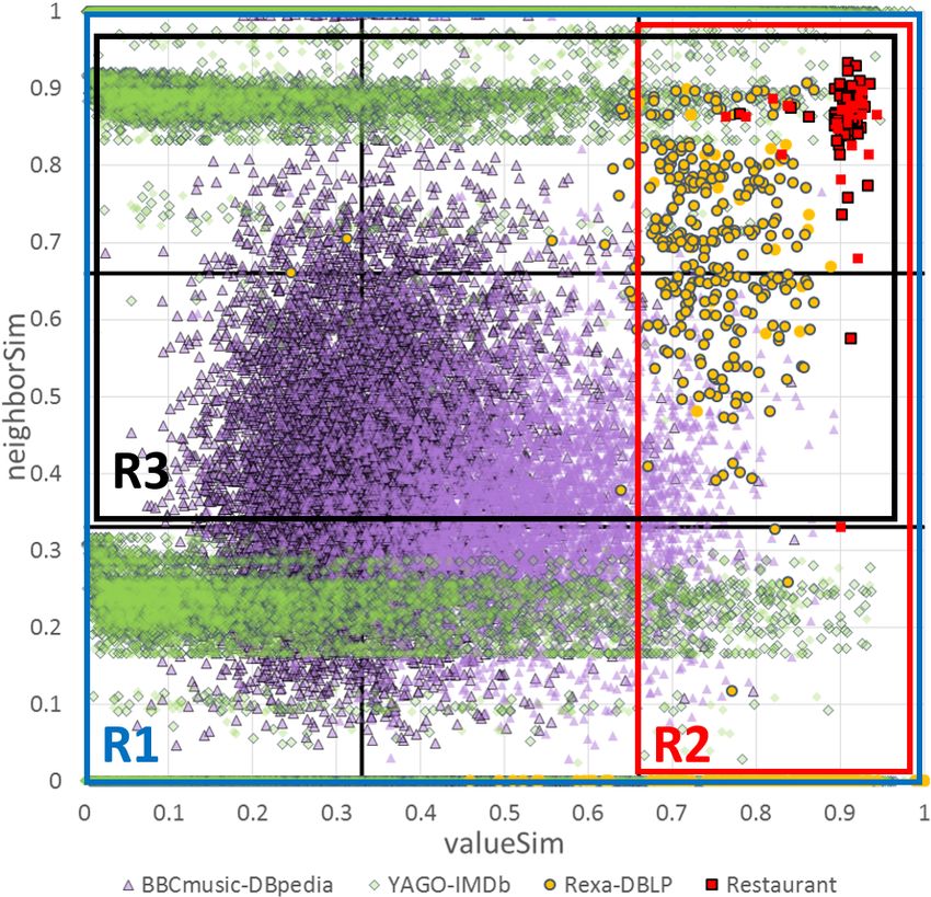
Figure 2: Value and neighbor similarity distribution of ing graph. We present an efficient algorithm for weighting and
matches in 4 datasets (see Table 1 for more details). then pruning the edges with low weights, which are unlikely to
correspond to matches. As opposed to existing disjunctive block-
ing schemes [3, 18], our disjunctive blocking is schema-agnostic
to infer that those descriptions are matching; they are strongly and requires no (semi-)supervised learning.
similar. However, we cannot be that sure about Restaurant1 and • We propose a non-iterative matching process that is imple-
Restaurant2, if we only look at their values. Those descriptions mented in Spark [36]. Unlike the data-driven convergence of ex-
are nearly similar and we have to look further at the similarity of isting systems (e.g., LINDA [4], SiGMa [21], RiMOM [31]), the
their neighbors (e.g, John Lake A and Jonny Lake) to verify that matching process of MinoanER involves a specific number of
they match. predefined generic, schema-agnostic matching rules (R1-R4) that
Figure 2 depicts both sources of similarity evidence (valueSim, traverse the blocking graph. First, we identify matches based on
neighborSim) for entities known to match (i.e., ground truth) in their name (R1). This is a very effective method that can be ap-
four benchmark datasets that are frequently used in the literature plied to all descriptions, regardless of their values or neighbor
(details in Table 1). Every dot corresponds to a matching pair similarity. Unlike the schema-based blocking keys of relational
of entities, and its shape denotes its origin KBs. The horizontal descriptions usually provided by domain experts, MinoanER auto-
axis reports the normalized value similarity (weighted Jaccard matically specifies distinctive names of entities from data statistics.
coefficient [21]) based on the tokens (i.e., single words in attribute Then, the value similarity is exploited to find matches with many
values) shared by a pair of descriptions, while the vertical one common and infrequent tokens, i.e., strongly similar matches
reports the maximum value similarity of their neighbors. The (R2). When value similarity is not high, nearly similar matches
value similarity of matching entities significantly varies across are identified based on both value and neighbors’ similarity using
different KBs. For strongly similar entities, e.g., with a value a threshold-free rank aggregation function (R3), as opposed to
similarity > 0.5, existing duplicate detection techniques work existing works that combine different matching evidence into an
well. However, a large part of the matching pairs of entities is aggregated score. Finally, reciprocal evidence of matching is ex-
covered by nearly similar entities, e.g., with a value similarity ploited as a verification of the returned results: only entities that
< 0.5. To resolve them, we need to additionally exploit evidence are mutually ranked in the top positions of their unified ranking
regarding the similarity of neighboring entities. lists are considered matches (R4). Figure 2 abstractly illustrates
This also requires revisiting the blocking (aka indexing) tech- the type of matching pairs that are covered by each matching rule.
niques used to reduce the number of candidate pairs [7]. To avoid • We experimentally compare the effectiveness of MinoanER
restricting candidate matches (i.e., descriptions placed on the against state-of-the-art methods using established benchmark data
same block) to strongly similar entities, we need to assess both that involve real KBs. The main conclusion drawn from our exper-
value and neighbor similarity of candidate matches. In essence, iments is that MinoanER achieves at least equivalent performance
rather than a unique indexing function, we need to consider a com- over KBs exhibiting a low Variety (e.g., those originating from
posite blocking that provides matching evidence from different a common data source like Wikipedia) even though the latter
sources, such as the content, the neighbors or even the names (e.g., make more assumptions about the input KBs (e.g., alignment of
rdfs:label) of entities. Creating massively parallelizable tech- relations); yet, MinoanER significantly outperforms state-of-the-
niques for processing the search space of candidate pairs formed art ER tools when matching KBs with high Variety. The source
by such composite blocking is an open research challenge. code and datasets used in our experimental study are publicly
Overall, the main requirements for Web-scale ER are: (i) iden- available3 .
tify both strongly and nearly similar matches, (ii) do not rely on a The rest of the paper is structured as follows: we introduce our
given schema, (iii) do not rely on domain experts for aligning re- value and neighbor similarities in Section 2, and we delve into the
lations and matching rules, (iv) develop non-iterative solutions to
avoid late convergence, and (v) scale to massive volumes of data. 2A preliminary, abridged version of this paper appeared in [13].
None of the existing ER frameworks proposed for the Web of 3 http://csd.uoc.gr/~vefthym/minoanER
374blocking schemes and the blocking graph that lie at the core of P ROOF. Please refer to the extended version of this paper5 . □
our approach in Section 3. Section 4 describes the matching rules
of our approach along with their implementation in Spark, while Note that valueSim has the following properties: (i) it is not a
Section 5 overviews the main differences with the state-of-the-art normalized metric, since it can take any value in [0, +∞), with 0
ER methods. We present our thorough experimental analysis in denoting the existence of no common tokens in the values of the
Section 6 and we conclude the paper in Section 7. compared descriptions. (ii) The maximum contribution of a single
common token between two descriptions is 1, in case this common
2 BASIC DEFINITIONS token does not appear in the values of any other entity description,
i.e., when EF E1 (t) · EF E2 (t) = 1. (iii) It is a schema-agnostic
Given a KB E, an entity description with a URI identifier i, de-
noted by ei ∈ E, is a set of attribute-value pairs about a real- similarity metric, as it disregards any schematic information6 .
world entity. When the identifier of an entity description e j ap-
pears in the values of another entity description ei , the corre- 2.2 Entity similarity based on neighbors
sponding attribute is called a relation and the corresponding In addition to value similarity, we exploit the relations between
value (e j ) a neighbor of ei . More formally, the relations of ei descriptions to find the matching entities of the compared KBs.
are defined as relations(ei ) = {p|(p, j) ∈ ei ∧ e j ∈ E}, while This can be done by aggregating the value similarity of all pairs
its neighbors as neiдhbors(ei ) = {e j |(p, j) ∈ ei ∧ e j ∈ E}. For of descriptions that are neighbors of the target descriptions.
example, for the Wikidata KB in the left side of Figure 1 we Given the potentially high number of neighbors that a descrip-
have: relations(Restaurant1) = {hasChef, territorial, inCountry}, tion might have, we propose considering only the most valuable
and neiдhbors(Restaurant1) = {John Lake A, Bray, United King- neighbors for computing the neighbor similarity between two
dom}. target descriptions. These are neighbors that are connected with
In the following, we exclusively consider clean-clean ER, i.e., the target descriptions via important relations, i.e., relations that
the sub-problem of ER that seeks matches among two duplicate- exhibit high support and discriminability. Intuitively, high support
free (clean) KBs. Thus, we simplify the presentation of our ap- for a particular relation p indicates that p appears in many entity
proach, but the proposed techniques can be easily generalized to descriptions, while high discriminability for p indicates that it has
more than two clean KBs or a single dirty KB, i.e., a KB that many distinct values. More formally:
contains duplicates.
Definition 2.2. The support of a relation p ∈ P in a KB E
|inst ances(p)|
2.1 Entity similarity based on values is defined as: support(p) = | E |2
, where instances(p) =
{(i, j)|ei , e j ∈ E ∧ (p, j) ∈ ei }.
Traditionally, similarity between entities is computed based on
their values. In our work, we apply a similarity measure based Definition 2.3. The discriminability of a relation p ∈ P in a
on the number and the frequency of common words between two |ob ject s(p)|
KB E is defined as: discriminability(p) = |inst ances(p)| , where
values4 .
objects(p) = {j |(i, j) ∈ instances(p)}.
Definition 2.1. Given two KBs, E1 and E2 , the value simi-
Overall, we combine support and discriminability via their
larity of two entity descriptions ei ∈ E1 , e j ∈ E2 is defined as:
harmonic mean in order to locate the most important relations.
valueSim(ei , e j )= t ∈t okens(ei )∩t okens(e j ) loд (E F (t1)·E F (t )+1) ,
Í
2 E1 E2
where EF E (t) = |{el |el ∈ E ∧ t ∈ tokens(el )}| stands for “En- Definition 2.4. The importance of a relation p ∈ P in a KB E
suppor t (p)·discr iminability(p)
tity Frequency”, which is the number of entity descriptions in E is defined as: importance(p) = 2· suppor t (p)+discr iminability(p) .
having token t in their values.
On this basis, we identify the most valuable relations and neigh-
This value similarity shares the same intuition as TF-IDF in bors for every single entity description (i.e., locally). We use
information retrieval. If two entities share many, infrequent to- topN relations(ei ) to denote the N relations in relations(ei ) with
kens, then they have high value similarity. On the contrary, very the maximum importance scores. Then, the best neighbors for
frequent words (resembling stopwords in information retrieval) ei are defined as: topNneiдhbors(ei ) = {nei |(p, nei ) ∈ ei ∧ p ∈
are not considered an important matching evidence, when they topN relations(ei )}.
are shared by two descriptions, and therefore, they only contribute Intuitively, strong matching evidence (high value similarity) for
insignificantly to the valueSim score. The number of common the important neighbors leads to strong matching evidence for the
words is accounted by the number of terms that are considered in target pair of descriptions. Hence, we formally define neighbor
the sum and the frequency of those words is given by the inverse similarity as follows:
Entity Frequency (EF), similar to the inverse Document Frequency
(DF) in information retrieval. Definition 2.5. Given two KBs, E1 and E2 , the neighbor simi-
larity of two entity descriptions ei ∈ E1 , e j ∈ E2 is:
Proposition 1. valueSim is a similarity metric, since it satisfies Õ
the following properties [5]: neiдhbor N Sim(ei , e j )= valueSim(nei , ne j ).
• valueSim(ei , ei ) ≥ 0, ne i ∈top N neiдhbor s(e i )
ne j ∈top N neiдhbor s(e j )
• valueSim(ei , e j ) = valueSim(e j , ei ),
• valueSim(ei , ei ) ≥ valueSim(ei , e j ), Proposition 2. neiдhbor N Sim is a similarity metric.
• valueSim(ei , ei ) = valueSim(e j , e j ) = valueSim(ei , e j ) ⇔ei =e j ,
5 http://csd.uoc.gr/~vefthym/DissertationEfthymiou.pdf
• valueSim(ei , e j ) + valueSim(e j , ez ) ≤ valueSim(ei , ez ) + 6 Note that our value similarity metric is crafted for the token-level noise in literal
valueSim(e j , e j ). values, rather than the character-level one. Yet, our overall approach is tolerant to
character-level noise, as verified by our extensive experimental analysis with real
4 We handle numbers and dates in the same way as strings, assuming string-dominated datasets that include it. The reason is that it is highly unlikely for matching entities
entities. to have character-level noise in all their common tokens.
375P ROOF. Given that neiдhbor N Sim is the sum of similarity met- distinct union of the block elements is the input entity collection
rics (valueSim), it is a similarity metric, too [5]. □ (i.e., all the descriptions from a set of input KBs). Formally:
Definition 3.1. Given an entity collection E, atomic blocking
Neither valueSim nor neiдhbor N Sim are normalized, since the is defined by an indexing function hkey for which the generated
number of terms that contribute in the sums is an important match- key key
ing evidence that can be mitigated if the values were normalized. blocks, B key ={b1 , . . . , bm }, satisfy the following conditions:
key key
(i) ∀ek , el ∈ bi : bi ∈ B key , okey (ek , el ) = true,
Example 2.6. Continuing our example in Figure 1, assume key key
that the best two relations for Restaurant1 and Restaurant2 are: (ii) ∀(ek , el ) : okey (ek , el )=true, ∃bi ∈ B key , ek , el ∈ bi ,
top2relations(Restaurant1) = {hasChef, territorial} and key
bi = E.
Ð
(iii)
top2relations(Restaurant2) = {headChef, county}. Then, bi
k ey
∈B k ey
top2neiдhbors(Restaurant1) = {John Lake A, Bray} and
Given that a single key is not enough for indexing loosely
top2neiдhbors(Restaurant2) = {Jonny Lake, Berkshire}, and
structured and highly heterogeneous entity descriptions, we need
neiдhbor 2Sim(Restaurant1, Restaurant2) =
to consider several keys that the indexing function will exploit to
valueSim(Bray, JonnyLake)+valueSim(John Lake A, Berkshire)
build different sets of blocks. Such a composite blocking method
+valueSim(Bray, Berkshire)+valueSim(John Lake A, Jonny Lake).
is characterized by a disjunctive co-occurrence function over the
Note that since we don’t have a relation mapping, we also consider
atomic blocks, and it is formally defined as:
the comparisons (Bray, JonnyLake) and (John Lake A, Berkshire).
Definition 3.2. Given an entity collection E, disjunctive block-
Entity Names. From every KB, we also derive the global top-k ing is defined by a set of indexing functions H , for which the gen-
attributes of highest importance, whose literal values act as names erated blocks B = B key satisfy the following conditions:
Ð
for any description ei that contains them. Their support is simply h k ey ∈H
defined as: support(p) = |subjects(p)|/|E |, where subjects(p) = (i) ∀ek , el ∈ b : b ∈ B, o H (ek , el ) = true,
{i |(i, j) ∈ instances(p)} [32]. Based on these statistics, function (ii) ∀(ek , el ) : o H (ek , el ) = true, ∃b ∈ B, ek , el ∈ b,
name(ei ) returns the names of ei , and Nx denotes all names in
where o H (ek , el ) = hk ey ∈H okey (ek , el ).
Ô
a KB Ex . In combination with topNneiдhbors(ei ), this function
covers both local and global property importance, exploiting both Atomic blocking can be seen as a special case of composite
the rare and frequent attributes that are distinctive enough to blocking, consisting of a singleton set, i.e., H = {hkey }.
designate matching entities.
3.1 Composite Blocking Scheme
3 BLOCKING To achieve a good trade-off between effectiveness and efficiency,
To enhance performance, blocking is typically used as a pre- our composite blocking scheme assesses the name and value sim-
processing step for ER in order to reduce the number of unneces- ilarity of the candidate matches in combination with similarity
sary comparisons, i.e., comparisons between descriptions that do evidence provided by their neighbors on important relations. We
not match. After blocking, each description can be compared only consider the blocks constructed for all entities ei ∈ E using the
to others placed within the same block. The desiderata of block- indexing function hi (·) both over entity names (∀n j ∈ names(ei ) :
ing are [6]: (i) to place matching descriptions in common blocks h N (n j )) and tokens (∀t j ∈ tokens(ei ) : hT (t j )). The composite
(effectiveness), and (ii) to minimize the number of suggested blocking scheme O of MinoanER is defined by the following
comparisons (time efficiency). However, efficiency dictates skip- disjunctive co-occurrence condition of any two entities ei , e j ∈ E:
ping many comparisons, possibly yielding many missed matches, O(ei , e j ) = o N (ei , e j ) ∨ oT (ei , e j )∨
( (ei′ ,e j′ )∈top N neiдhbor s(ei )×top N neiдhbor s(e j ) oT (ei′, e j′ )), where
Ô
which in turn implies low effectiveness. Thus, the main objective
of blocking is to achieve a good trade-off between minimizing the o N , oT is the co-occurrence function applied on names and to-
number of suggested comparisons and minimizing the number of kens, respectively. Intuitively, two entities are placed in a common
missed matches [7]. block, and are then considered candidate matches, if at least one
In general, blocking methods are defined over key values that of the following three cases holds: (i) they have the same name,
can be used to decide whether or not an entity description could be which is not used by any other entity, in which case the common
placed in a block using an indexing function [7]. The ‘uniqueness’ block contains only those two entities, or (ii) they have at least
of key values determines the number of entity descriptions placed one common word in any of their values, in which case the size of
in the same block, i.e., which are considered as candidate matches. the common block is given by the product of the Entity Frequency
More formally, the building blocks of a blocking method can be (EF ) of the common term in the two input collections, or (iii)
defined as [3]: their top neighbors share a common word in any of their values.
• An indexing function hkey : E → 2B is a unary function that, Note that token blocking (i.e., hT ) allows for deriving valueSim
when applied to an entity description using a specific blocking from the size of blocks shared by two descriptions. As a result,
key, it returns as a value the subset of the set of all blocks B, under no additional blocks are needed to assess neighbor similarity of
which the description will be indexed. candidate entities: token blocking is sufficient also for estimating
• A co-occurrence function okey : E × E → {true, f alse} is a neiдhbor Nsim according to Definition 2.5.
binary function that, when applied to a pair of entity descriptions,
it returns ‘true’ if the intersection of the sets of blocks produced by 3.2 Disjunctive Blocking Graph
the indexing function on its arguments, is non-empty, and ‘false’ The disjunctive blocking graph G is an abstraction of the dis-
otherwise; okey (ek , el ) = true iff hkey (ek ) ∩ hkey (el ) , ∅. junctive co-occurrence condition of candidate matches in blocks.
In this context, each pair of descriptions whose co-occurrence Nodes represent candidates from our input entity descriptions,
function returns ‘true’ shares at least one common block, and the while edges represent pairs of candidates for which at least one
3763.3 Graph Weighting and Pruning Algorithms
Each edge in the blocking graph represents a suggested compari-
son between two descriptions. To reduce the number of compar-
isons suggested by the disjunctive blocking graph, we keep for
each node the K edges with the highest β and the K edges with
the highest γ weights, while pruning edges with trivial weights
(i.e., (α, β, γ )=(0,0,0)), since they connect descriptions unlikely to
match. Given that nodes vi and v j may have different top K edges
based on β or γ , we consider each undirected edge in G as two
directed ones, with the same initial weights, and perform pruning
on them.
Example 3.5. Figure 3(b) shows the pruned version of the
graph in Figure 3(a). Note that the blocking graph is only a con-
ceptual model, which we do not materialize; we retrieve any nec-
essary information from computationally cheap inverted indices.
The process of weighting and pruning the edges of the dis-
Figure 3: (a) Parts of the disjunctive blocking graph corre- junctive blocking graph is described in Algorithm 1. Initially, the
sponding to Figure 1, and (b) the corresponding blocking graph contains no edges. We start adding edges by checking the
graph after pruning. name blocks B N (Lines 5-9). For each name block b that contains
exactly two entities, one from each KB, we create an edge with
of the co-occurrence conditions is ‘true’. Each edge is actually α=1 linking those entities (note that in Algorithm 1, b k , k∈{1, 2},
labeled with three weights that quantify similarity evidence on denotes the sub-block of b that contains the entities from Ek ,
names, tokens and neighbors of candidate matches. Specifically, i.e., b k ⊆Ek ). Then, we compute the β weights (Lines 10-14) by
the disjunctive blocking graph of MinoanER is a graph G = running a variation of Meta-blocking [27], adapted to our value
(V , E, λ), with λ assigning to each edge a label (α, β, γ ), where similarity metric (Definition 2.1). Next, we keep for each entity,
α is ‘1’ if o N (ei , e j ) is true and the name block in which ei , e j its connected nodes from the K edges with the highest β (Lines 15-
co-occur is of size 2, and ‘0’ otherwise, β = valueSim(ei , e j ), and 18). Line 20 calls the procedure for computing the top in-neighbors
γ = neiдhbor N Sim(ei , e j ). More formally: of each entity, which operates as follows: first, it identifies each
entity’s topNneiдbors (Lines 36-43) and then, it gets their reverse;
Definition 3.3. Given a block collection B = hk ey ∈H B key ,
Ð
for every entity ei , we get the entities topInN eiдhbors[i] that have
produced by a set of indexing functions H , the disjunctive block-
ei as one of their topN neiдhbors (Lines 44-47). This allows for
ing graph for an entity collection E, is a graph G = (V , E, λ),
estimating the γ weights according to Definition 2.5. To avoid
where each node vi ∈ V represents a distinct description ei ∈ E,
re-computing the value similarities that are necessary for the γ
and each edge ∈ E represents a pair ei , e j ∈ E for which
computations, we exploit the already computed βs. For each pair
O(ei , e j ) = ‘true ′ ; O(ei , e j ) is a disjunction of the atomic co-
of entities ei ∈ E1 , e j ∈ E2 that are connected with an edge with
occurrence functions ok defined along with H , and λ : E → R n is β > 0, we assign to each pair of their inN eiдhbors, (ini , in j ), a
a labeling function assigning a tuple [w 1 , . . . , w n ] to each edge, partial γ equal to this β (Lines 20-27). After iterating over all
where w k is a weight associated with each co-occurrence function such entity pairs ei , e j , we get their total neighbor similarity, i.e.,
ok of H . γ [i, j] = neiдhbor Nsim(ei , e j ). Finally, we keep for each entity,
Definition 3.3 covers the cases of an entity collection E being its K neighbors with the highest γ (Lines 28-33).
composed of one, two, or more KBs. When matching k KBs, as- The time complexity of Algorithm 1 is dominated by the pro-
suming that all of them are clean, the disjunctive blocking graph cessing of value evidence, which iterates twice over all compar-
is k-partite, with each of the k KBs corresponding to a different isons in the token blocks BT . In the worst-case, this results in
independent set of nodes, i.e., there are only edges between de- one computation for every pair of entities, i.e., O(|E1 | · |E2 |). In
scriptions from different KBs. The only information needed to practice, though, we bound the number of computations by remov-
match multiple KBs is to which KB every description belongs, so ing excessively large blocks that correspond to highly frequent
as to add it to the corresponding independent set. Similarly, the tokens (e.g., stop-words). Following [27], this is carried out by
disjunctive blocking graph covers dirty ER, as well. Block Purging [26], which ensures that the resulting blocks in-
volve two orders of magnitude fewer comparisons than the brute-
Example 3.4. Consider the graph of Figure 3(a), which is part force approach, without any significant impact on recall. This
of the disjunctive blocking graph generated from Figure 1. John complexity is higher than that of name and neighbor evidence,
Lake A and Jonny Lake have a common name (“J. Lake”), and which are both linearly dependent on the number of input entities.
there is no other entity having this name, so there is an edge The former involves a single iteration over the name blocks B N ,
connecting them with α = 1. Bray and Berkshire have common, which amount to |N1 ∩ N2 |, as there is one block for every name
quite infrequent tokens in their values, so their similarity (β in shared by E1 and E2 . For neighbor evidence, Algorithm 1 checks
the edge connecting them) is quite high (β = 1.2). Since Bray is all pairs of N neighbors between every entity ei and its K most
a top neighbor of Restaurant1 in Figure 1, and Berkshire is a top value-similar descriptions, performing K · N 2 · (|E1 | + |E2 |) oper-
neighbor of Restaurant2, there is also an edge with a non-zero ations; the cost of estimating the top in-neighbors for each entity
γ connecting Restaurant1 with Restaurant2. The γ score of this is lower, dominated by the ordering of all relations in E1 and E2
edge (1.6) is the sum of the β scores of the edges connecting Bray (i.e., |Rmax | · loд|Rmax |), where |Rmax | stands for the maximum
with Berkshire (1.2), and John Lake A with Jonny Lake (0.4). number of relations in one of the KBs.
377Algorithm 1: Disjunctive Blocking Graph Construction. Algorithm 2: Non-iterative Matching.
Input: E1, E2 , the blocks from name and token blocking, B N and BT Input: E1, E2 , The pruned, directed disjunctive blocking graph G .
Output: A disjunctive blocking graph G . Output: A set of matches M .
1 procedure getCompositeBlockingGraph( E1, E2, B N , BT ) 1 M ← ∅; // The set of matches
2 V ← E1 ∪ E2 ;
// Name Matching Value (R1)
3 E ← ∅;
2 for < v i , v j > ∈ G .E do
4 W ← ∅; // init. to (0, 0, 0) 3 if G .W .дet (α, < v i , v j >) = 1 then
// Name Evidence 4 M ← M ∪ (e i , e j );
5 for b ∈ B N do
6 if |b 1 | · |b 2 | = 1 then // only 1 comparison in b // Value Matching Value (R2)
7 e i ←b 1 .дet (0), e j ←b 2 .дet (0) ; // entities in b 5 for v i ∈ G .V do
8 E ← E ∪ {< v i , v j > }; 6 if e i ∈ E1 \ M then // check the smallest KB for
9 W ← W .set (α, < v i , v j >, 1); efficiency
7 v j ← ar дmaxvk ∈G .V G .W .дet (β, < v i , v k >) ; // top
// Value Evidence candidate
10 for e i ∈ E1 do 8 if G .W .дet (β, < v i , v j >) ≥ 1 then
11 β [] ← ∅ ; // value weights wrt all e j ∈ E2 9 M ← M ∪ (e i , e j );
12 for b ∈ BT ∧ b ∩ e i , ∅ do
13 for e j ∈ b 2 do // e j ∈ E2 // Rank Aggregation Matching Value (R3)
14 β [j]←β [j]+1/loд2 ( |b 1 | · |b 2 | +1) ; // valueSim 10 for v i ∈ G .V do
11 if e i ∈ E1 ∪ E2 \ M then
15 V alueCandidat es ← дetT opCandidat es(β [], K );
12 aдд[] ← ∅; // Aggregate scores, init. zeros
16 for e j ∈ V alueCandidat es do
17 E ← E ∪ {< v i , v j > }; 13 valCands ← G .valCand (e i ) ; // nodes linked to e i
in decr. β
18 W ← W .set (β, < v i , v j >, β [j]);
14 r ank ← |valCands | ;
19 for e i ∈ E2 do . . . ; // ...do the same for E2 15 for e j ∈ valCands do
16 aдд[e i ].updat e(e j , θ · r ank /|valCands |);
// Neighbor Evidence
17 r ank ← r ank − 1;
20 inN eiдhbor s[] ← дetT opI nN eiдhbor s(E1, E2 );
21 γ [][] ← ∅ ; // neighbor weights wrt all e i , e j ∈ V 18 nдbCands ← G .nдbCand (e i ) ; // nodes linked to e i
22 for e i ∈ E1 do in decr. γ
23 for e j ∈ E2 , s.t. W .дet (β, < v i , v j >) > 0 do 19 r ank ← |nдbCands | ;
24 for in j ∈ inN eiдhbor s[j] do 20 for e j ∈ nдbCands do
25 for in i ∈ inN eiдhbor s[i] do // neighborNSim 21 aдд[e i ].updat e(e j , (1 − θ ) · r ank /|nдbCands |);
26 γ [i][j] ← γ [i][j] + W .дet (β, < n i , n j >); 22 r ank ← r ank − 1;
23 M ← M ∪ (e i , дetT opCandidat e(aдд[e i ]));
27 for e i ∈ E2 do . . . ; // ...do the same for E2
28 for e i ∈ E1 do // Reciprocity Matching Value (R4)
29 N eiдhbor Candidat es ← дetT opCandidat es(γ [i][], K ); 24 for (e i , e j ) ∈ M do
30 for e j ∈ N eiдhbor Candidat es do 25 if < v i , v j >< G .E ∨ < v j , v i >< G .E then
31 E ← E ∪ {< v i , v j > }; 26 M ← M \ (e i , e j );
32 W .set (γ , < v i , v j >, γ [i][j]);
27 return M ;
33 for e i ∈ E2 do . . . ; // ...do the same for E2
34 return G = (V , E, W );
35 procedure getTopInNeighbors( E1, E2 ) match, if they, and only they, have the same name n. Thus, R1
36 t op N eiдhbor s[] ← ∅ ; // one list for each entity traverses G and for every edge with α = 1, it updates the
37 дlobalOr der ← sort E1 ’s relations by importance; set of matches M with the corresponding descriptions (Lines 2-4
38 for e ∈ E1 do
39 localOr der (e)←r el at ions(e).sor t By(дlobalOr der );
in Alg. 2). All candidates matched by R1 are not examined by the
40 t op N r el at ions ← localOr der (e).t op N ; remaining rules.
41 for (p, o) ∈ e , where p ∈ t op N r el at ions do Value Matching Rule (R2). It presumes that two entities match,
42 t op N eiдhbor s[e].add(o);
if they, and only they, share a common token t, or, if they share
43 for e i ∈ E2 do . . . ; // ...do the same for E2 many infrequent tokens. Based on Definition 2.1, R2 identifies
44 t opI nN eiдhbor s[]←∅; // the reverse of topNeighbors pairs of descriptions with high value similarity (Lines 5-9). To
45 for e ∈ E1 ∪ E2 do
46 for ne ∈ t op N eiдhbor s[e] do this end, it goes through every node vi of G and checks whether
47 t opI nN eiдhbor s[ne].add (e); the corresponding description stems from the smaller in size KB,
48 return t opI nN eiдhbor s ;
for efficiency reasons (fewer checks), but has not been matched
yet. In this case, it locates the adjacent node v j with the maximum
β weight (Line 7). If β ≥ 1, R2 considers the pair (ei , e j ) to be
a match. Matches identified by R2 will not be considered in the
4 NON-ITERATIVE MATCHING PROCESS sequel.
Our matching method receives as input the disjunctive blocking Rank Aggregation Matching Rule (R3). This rule identifies fur-
graph G and performs four steps – unlike most existing works, ther matches for candidates whose value similarity is low (β < 1),
which involve a data-driven iterative process. In every step, a yet their neighbor similarity (γ ) could be relatively high. In this
matching rule is applied with the goal of extracting new matches respect, the order of candidates rather than their absolute similarity
from the edges of G by analyzing their weights. The functionality values are used. Its functionality appears in Lines 10-23 of Algo-
of our algorithm is outlined in Algorithm 2. Next, we describe its rithm 2. In essence, R3 traverses all nodes of G that correspond to
rules in the order they are applied: a description that has not been matched yet. For every such node
Name Matching Rule (R1). The matching evidence of R1 comes vi , it retrieves two lists: the first one contains adjacent edges with
from the entity names. It assumes that two candidate entities a non-zero β weight, sorted in descending order (Line 13), while
3784.1 Implementation in Spark
Figure 4 shows the architecture of MinoanER implementation in
Spark. Each process is executed in parallel for different chunks of
input, in different Spark workers. Each dashed edge represents a
synchronization point, at which the process has to wait for results
produced by different data chunks (and different Spark workers).
In more detail, Algorithm 1 is adapted to Spark by applying
name blocking simultaneously with token blocking and the ex-
traction of top neighbors per entity. Name blocking and token
blocking produce the sets of blocks B N and BT , respectively,
which are part of the algorithm’s input. The processing of those
blocks in order to estimate the α and β weights (Lines 5-9 for B N
and Lines 10-18 for BT ) takes place during the construction of
the blocks. The extraction of top neighbors per entity (Line 20)
runs in parallel to these two processes and its output, along with
Figure 4: The architecture of MinoanER in Spark. the β weights, is given to the last part of the graph construction,
which computes the γ weights for all entity pairs with neighbors
the second one includes the adjacent edges sorted in decreasing
co-occuring in at least one block (Lines 21-33).
non-zero γ weights (Line 18). Then, R3 aggregates the two lists
To minimize the overall run-time, Algorithm 2 is adapted to
by considering the normalized ranks of their elements: assuming
Spark as follows: R1 (Lines 2-4) is executed in parallel with
the size of a list is K, the first candidate gets the score K/K, the
name blocking and the matches it discovers are broadcasted to be
second one (K − 1)/K, while the last one 1/K. Overall, each ad-
excluded from subsequent rules. R2 (Lines 5-9) runs after both
jacent node of vi takes a score equal to the weighted summation
R1 and token blocking have finished, while R3 (Lines 10-23) runs
of its normalized ranks in the two lists, as determined through the
after both R2 and the computation of neighbor similarities have
trade-off parameter θ ∈ (0, 1) (Lines 16 & 21): the scores of the β
been completed, skipping the already identified (and broadcasted)
list are weighted with θ and those of the γ list with 1-θ . At the end,
matches. R4 (Lines 24-26) runs in the end, providing the final,
vi is matched with its top-1 candidate match v j , i.e., the one with
filtered set of matches. Note that during the execution of every
the highest aggregate score (Line 23). Intuitively, R3 matches ei
rule, each Spark worker contains only the partial information of
with e j , when, based on all available evidence, there is no better
the disjunctive blocking graph that is necessary to find the match
candidate for ei than e j .
of a specific node (i.e., the corresponding lists of candidates based
Reciprocity Matching Rule (R4). It aims to clean the matches on names, values, or neighbors).
identified by R1, R2 and R3 by exploiting the reciprocal edges of
G. Given that the originally undirected graph G becomes directed
after pruning (as it retains the best edges per node), a pair of nodes 5 RELATED WORK
vi and v j are reciprocally connected when there are two edges To the best of our knowledge, there is currently no other Web-
between them, i.e., an edge from vi to v j and an edge from v j scale ER framework that is fully automated, non-iterative, schema-
to vi . Hence, R4 aims to improve the precision of our algorithm agnostic and massively parallel, at the same time. For example,
based on the rationale that two entities are unlikely to match, when WInte.r [22] is a framework that performs multi-type ER, also
one of them does not even consider the other to be a candidate incorporating the steps of blocking, schema-level mapping and
for matching. Intuitively, two entity descriptions match, only if data fusion. However, it is implemented in a sequential fashion
both of them “agree” that they are likely to match. R4 essentially and its solution relies on a specific level of structuredness, i.e., on a
iterates over all matches detected by the above rules and discards schema followed by the instances to be matched. Dedoop [20] is a
those missing any of the two directed edges (Lines 24-26), acting highly scalable ER framework that comprises the steps of blocking
more like a filter for the matches suggested by the previous rules. and supervised matching. However, it is the user that is responsible
Given a pruned disjunctive blocking graph, every rule can be for selecting one of the available blocking and learning methods
formalized as a function that receives a pair of entities and returns and for fine-tuning their internal parameters. This approach is
true (T ) if the entities match according to the rule’s rationale, or also targeting datasets with a predefined schema. Dedupe [16]
false (F ) otherwise, i.e., Rn : E1 × E2 → {T , F }. In this context, is a scalable open-source Python library (and a commercial tool
we formally define the MinoanER matching process as follows: built on this library) for ER; however, it is not fully automated, as
it performs active learning, relying on human experts to decide
Definition 4.1. The non-iterative matching of two KBs E1 , for a first few difficult matching decisions. Finally, we consider
E2 , denoted by the Boolean matrix M(E1 , E2 ), is defined as a progressive ER (e.g., [1]) orthogonal to our approach, as it aims
filtering problem of the pruned disjunctive blocking graph G: to retrieve as many matches as possible as early as possible.
M(ei , e j ) = (R1(ei , e j ) ∨ R2(ei , e j ) ∨ R3(ei , e j )) ∧ R4(ei , e j ). In this context, we compare MinoanER independently to state-
The time complexity of Algorithm 2 is dominated by the size of-the-art matching and blocking approaches for Web data.
of the pruned blocking graph G it receives as input, since R1, R2 Entity Matching. Two types of similarity measures are com-
and R3 essentially go through all directed edges in G (in practice, monly used for entity matching [21, 31]. (i) Value-based simi-
though, R1 reduces the edges considered by R2 and R3, and so larities (e.g., Jaccard, Dice) usually assess the similarity of two
does R2 for R3). In the worst case, G contains 2K directed edges descriptions based on the values of specific attributes. Our value
for every description in E1 ∪ E2 , i.e., |V |max = 2 · K · (|E1 | + |E2 |). similarity is a variation of ARCS, a Meta-blocking weighting
Thus, the overall complexity is linear with respect to the number scheme [12], which disregards any schema information and con-
of input descriptions, i.e., O(|E1 |+|E2 |), yielding high scalability. siders each entity description as a bag of words. Compared to
379ARCS, though, we focus more on the number than the frequency the results of multiple blocks, an iterative message-passing frame-
of common tokens between two descriptions. (ii) Relational simi- work is employed. Rather than a block-level synchronization, the
larity measures additionally consider neighbor similarity by ex- MinoanER parallel computations in Spark require synchronization
ploiting the value similarity of (some of) the entities’ neighbors. only across the 4 generic matching rules (see Figure 4).
Based on the nature of the matching decision, ER can be char- Regarding the matching rules, the ones employed by MinoanER
acterized as pairwise or collective. The former relies exclusively based on values and names are similar to rules that have already
on the value similarity of descriptions to decide if they match been employed in the literature individually (e.g., in [21, 23, 31]).
(e.g., [20]), while the latter iteratively updates the matching deci- In this work, we use a combination of those rules for the first time,
sion for entities by dynamically assessing the similarity of their also introducing a novel rank aggregation rule to incorporate value
neighbors (e.g., [2]). Typically, the starting point for this similarity and neighbor matching evidence. Finally, the idea of reciprocity
propagation is a set of seed matches identified by a value-based has been applied to enhance the results of Meta-blocking [28], but
blocking. was never used in matching.
For example, SiGMa [21] starts with seed matches having iden- Blocking. Blocking techniques for relational databases [6] rely
tical entity names. Then, it propagates the matching decisions on blocking keys defined at the schema-level. For example, the
on the ‘compatible’ neighbors, which are linked with pre-aligned Sorted Neighborhood approach orders entity descriptions accord-
relations. For every new matched pair, the similarities of the neigh- ing to a sorting criterion and performs blocking based on it; it is ex-
bors are recomputed and their position in the priority queue is pected that matching descriptions will be neighbors after the sort-
updated. LINDA [4] differs by considering as compatible neigh- ing, so neighbor descriptions constitute candidate matches [17].
bors those connected with relations having similar names (i.e., Initially, entity descriptions are lexicographically ordered based
small edit distance). However, this requirement rarely holds in the on their blocking keys. Then, a window, resembling a block, of
extreme schema heterogeneity of Web data. RiMOM-IM [23, 31] fixed length slides over the ordered descriptions, each time com-
is a similar approach, introducing the following heuristic: if two paring only the contents of the window. An adaptive variation of
matched descriptions e 1 , e 1′ are connected via aligned relations r the sorted neighborhood method is to dynamically decide on the
and r ′ and all their entity neighbors via r and r ′ , except e 2 and e 2′ , size of the window [35]. In this case, adjacent blocking keys in
have been matched, then e 2 and e 2′ are also considered matches. the sorted descriptions that are significantly different from each
All these methods employ Unique Mapping Clustering for other, are used as boundary pairs, marking the positions where
detecting matches: they place all pairs into a priority queue, in one window ends and the next one starts. Hence, this variation cre-
decreasing similarity. At each iteration, the top pair is considered ates non-overlapping blocks. In a similar line of work, the sorted
a match, if none of its entities has been already matched. The blocks method [11] allows setting the size of the window, as well
process ends when the top pair has a similarity lower than t. as the degree of desired overlap.
MinoanER employs Unique Mapping Clustering, too. Yet, Another recent schema-based blocking method uses Maximal
it differs from SiGMa, LINDA and RiMOM-IM in five ways: Frequent Itemsets (MFI) as blocking keys [19] – an itemset can
(i) the matching process iterates over the disjunctive blocking be a set of tokens. Abstractly, each MFI of a specific attribute
graph, instead of the initial KBs. (ii) MinoanER employs statistics in the schema of a description defines a block, and descriptions
to automatically discover distinctive entity names and important containing the tokens of an MFI for this attribute are placed in a
relations. (iii) MinoanER exploits different sources of matching common block. Using frequent itemsets to construct blocks may
evidence (values, names and neighbors) to statically identify can- significantly reduce the number of candidates for matching pairs.
didate matches already from the step of blocking. (iv) MinoanER However, since many matching descriptions share few, or even
does not aggregate different similarities in one similarity score; no common tokens, further requiring that those tokens are parts
instead, it uses a disjunction of the different evidence it considers. of frequent itemsets is too restrictive. The same applies to the
(v) MinoanER is a static collective ER approach, in which all requirement for a-priori schema knowledge and alignment, thus
sources of similarity are assessed only once per candidate pair. By resulting in many missed matches in the Web of Data.
considering a composite blocking not only on the value but also Although blocking has been extensively studied for tabular
on the neighbors similarity, we discover in a non-iterative way data, the proposed approaches cannot be used for the Web of Data,
most of the matches returned by the data-driven convergence of since their blocking keys rely on the existence of a global schema.
existing systems, or even more (see Section 6). However, the use of schema-based blocking keys is inapplicable
PARIS [33] uses a probabilistic model to identify matches, to the Web of Data, due to its extreme schema heterogeneity [15]:
based on previous matches and the functional nature of entity entity descriptions do not follow a fixed schema, as even a single
relations. A relation is considered functional if, for a source entity, description typically uses attributes defined in multiple LOD vo-
there is only one destination entity. If r (x, y) is a function in one cabularies. In this context, schema-agnostic blocking methods are
KB and r (x, y ′ ) a function in another KB, then y and y ′ are con- needed instead. Yet, the schema-agnostic functionality of most
sidered matches. The functionality of a relation and the alignment blocking methods requires extensive fine-tuning to achieve high
of relations along with previous matching decisions determine effectiveness [29]. The only exception is token blocking, which
the decisions in subsequent iterations. Unlike MinoanER, PARIS is completely parameter-free [26]. Another advantage of token
cannot deal with structural heterogeneity, while it targets both blocking is that it allows for computing value similarity from
ontology and instance matching. its blocks, as they contain entities with identical blocking keys –
Finally, [30] parallelizes the collective ER approach of [2], re- unlike other methods like Dedoop [20] and Sorted Neighborhood
lying on a black-box matching and exploits a set of heuristic rules [17], whose blocks contain entities with similar keys.
for structured entities. It essentially runs multiple instances of SiGMa [21] considers descriptions with at least two common
the matching algorithm in subsets of the input entities (similar tokens as candidate matches, which is more precise than our token
to blocks), also keeping information for all the entity neighbors, blocking, but misses more matches. The missed matches will be
needed for similarity propagation. Since some rules may require considered in subsequent iterations, if their neighbor similarity is
380Table 1: Dataset statistics. Table 2: Block statistics.
Restau- Rexa- BBCmusic- YAGO- Restaurant Rexa- BBCmusic- YAGO-
rant DBLP DBpedia IMDb DBLP DBpedia IMDb
E1 entities 339 18,492 58,793 5,208,100 |B N | 83 15,912 28,844 580,518
E2 entities 2,256 2,650,832 256,602 5,328,774 |BT | 625 22,297 54,380 495,973
E1 triples 1,130 87,519 456,304 27,547,595 | |B N | | 83 6.71 ·107 1.25 ·107 6.59 ·106
E2 triples 7,519 14,936,373 8,044,247 47,843,680 | |BT | | 1.80 ·103 6.54 ·108 1.73 ·108 2.28 ·1010
E1 av. tokens 20.44 40.71 81.19 15.56 | E1 | · | E2 | 7.65 ·105 4.90 ·1010 1.51 ·1010 2.78 ·1013
E2 av. tokens 20.61 59.24 324.75 12.49 Precision 4.95 1.81 ·10−4 0.01 2.46 ·10−4
E1 / E2 attributes 7/7 114 / 145 27 / 10,953 65 / 29 Recall 100.00 99.77 99.83 99.35
E1 / E2 relations 2/2 103 / 123 9 / 953 4 / 13 F1 9.43 3.62 ·10−4 0.02 4.92 ·10−4
E1 / E2 types 3/3 4 / 11 4 / 59,801 11,767 / 15
E1 / E2 vocab. 2/2 4/4 4/6 3/1
Matches 89 1,309 22,770 56,683 easy to resolve, Table 1 shows that it exhibits the greatest differ-
ence with respect to the size of the KBs to be matched (DBLP is
strong, whereas MinoanER identifies such matches from the step of 2 orders of magnitude bigger than Rexa in terms of descriptions,
blocking. RiMOM-IM [31] computes the tokens’ TF-IDF weights, and 3 orders of magnitude in terms of triples).
takes the top-5 tokens of each entity, and constructs a block for BBCmusic-DBpedia [14] contains descriptions of musicians,
each one, along with the attribute this value appears. Compared to bands and their birthplaces, from BBCmusic and the BTC2012
the full automation of MinoanER, this method requires attribute version of DBpedia10 . In our experiments, we consider only en-
alignment. [25] iteratively splits large blocks into smaller ones by tities appearing in the ground truth, as well as their immediate
adding attributes to the blocking key. This leads to a prohibitive in- and out-neighbors. The most challenging characteristic of this
technique for voluminous KBs of high Variety. dataset is the high heterogeneity between its two KBs in terms
Disjunctive blocking schemes have been proposed for KBs of of both schema and values: DBpedia contains ∼11,000 different
high [18] and low [3] levels of schema heterogeneity. Both meth- attributes, ∼60,000 entity types, 953 relations, the highest number
ods, though, are of limited applicability, as they require labelled of different vocabularies (6), while using on average 4 times more
instances for their supervised learning. In contrast, MinoanER tokens than BBCmusic to describe an entity. The latter feature
copes with the Volume and Variety of the Web of Data, through an means that all normalized, set-based similarity measures like Jac-
unsupervised, schema-agnostic, disjunctive blocking. card fail to identify such matches, since a big difference in the
Finally, LSH blocking techniques (e.g., [24]) hash descriptions token set sizes yields low similarity values (see Figure 2). A thor-
multiple times, using a family of hash functions, so that similar ough investigation has shown that in the median case, an entity
descriptions are more likely to be placed into the same bucket description in this dataset contains only 2 words in its values that
than dissimilar ones. This requires tuning a similarity threshold are used by both KBs [14].
between entity pairs, above which they are considered candidate YAGO-IMDb [33] contains descriptions of movie-related enti-
matches. This tuning is non-trivial, especially for descriptions ties (e.g., actors, directors, movies) from YAGO11 and IMDb12 .
from different domains, while its effectiveness is limited for nearly Figure 2 shows that a large number of matches in this dataset has
similar entities (see Figure 2). low value similarity, while a significant number has high neighbor
similarity. Moreover, this is the biggest dataset in terms of entities
6 EXPERIMENTAL EVALUATION and triples, challenging the scalability of ER tools, while it is the
In this section, we thoroughly compare MinoanER to state-of-the- most balanced pair of KBs with respect to their relative size.
art tools and a heavily fine-tuned baseline method. Baselines. In our experiments, we compare MinoanER against
Experimental Setup. All experiments were performed on top four state-of-the-art methods: SiGMa, PARIS, LINDA and Ri-
of Apache Spark v2.1.0 and Java 8, on a cluster of 4 Ubuntu MOM. PARIS is openly available, so we ran its original imple-
16.04.2 LTS servers. Each server has 236GB RAM and 36 Intel(R) mentation. For the remaining tools, we report their performance
Xeon(R) E5-2630 v4 @2.20GHz CPU cores. from the original publications13 . We also consider BSL, a custom
Datasets. We use four established benchmark datasets with en- baseline method that receives as input the disjunctive blocking
tities from real KBs. Their technical characteristics appear in graph G, before pruning, and compares every pair of descriptions
Table 1. All KBs contain relations between the described entities. connected by an edge in G. The resulting similarities are then
Restaurant7 contains descriptions of restaurants and their ad- processed by Unique Mapping Clustering. Unlike MinoanER,
dresses from two different KBs. It is the smallest dataset in terms though, BSL disregards all evidence from entity neighbors, relying
of the number of entities, triples, entity types8 , as well as the exclusively on value similarity. Yet, it optimizes its performance
one using the smallest number of vocabularies. We use it for two through a series of well-established string matching methods that
reasons: (i) it is a popular benchmark, created by the Ontology undergo extensive fine-tuning on the basis of the ground-truth.
Alignment Evaluation Initiative, and (ii) it offers a good example In more detail, we consider numerous configurations for the
of a dataset with very high value and neighbor similarity between four parameters of BSL in order to maximize its F1: (i) The
matches (Figure 2), involving the easiest pair of KBs to resolve. schema-agnostic representation of the values in every entity. BSL
Rexa-DBLP9 contains descriptions of publications and their uses token n-grams for this purpose, with n ∈ {1, 2, 3}, thus repre-
authors. The ground truth contains matches between both publica- senting every resource by the token uni-/bi-/tri-grams that appear
tions and authors. This dataset contains strongly similar matches in
10 datahub.io/dataset/bbc-music,
terms of values and neighbors (Figure 2). Although it is relatively km.aifb.kit.edu/projects/btc-2012/
11 www.yago-knowledge.org
7 http://oaei.ontologymatching.org/2010/im/ 12 www.imdb.com
8 Extracted using the attribute w3.org/1999/02/22-rdf-syntax-ns#type. 13 RiMOM-IM [31] is openly available, but no execution instructions were made
9 oaei.ontologymatching.org/2009/instances/ available to us.
381You can also read