Palette-based image decomposition, harmonization, and color transfer - arXiv
←
→
Page content transcription
If your browser does not render page correctly, please read the page content below
Palette-based image decomposition, harmonization, and color transfer
                                         JIANCHAO TAN, George Mason University
                                         JOSE ECHEVARRIA, Adobe Research
                                         YOTAM GINGOLD, George Mason University
arXiv:1804.01225v3 [cs.GR] 20 Jun 2018

                                         Fig. 1. Our palette-based color harmony template is able to express harmonization and various other color operations in a concise manner. Our edits make use
                                         of a new, extremely efficient image decomposition technique based on the 5D geometry of RGBXY-space.

                                         We present a palette-based framework for color composition for visual                       1   INTRODUCTION
                                         applications. Color composition is a critical aspect of visual applications                 Color composition is critical in visual applications in art, design,
                                         in art, design, and visualization. The color wheel is often used to explain
                                                                                                                                     and visualization. Over the centuries, different theories about how
                                         pleasing color combinations in geometric terms, and, in digital design, to
                                         provide a user interface to visualize and manipulate colors.
                                                                                                                                     colors interact with each other have been proposed [Westland et al.
                                            We abstract relationships between palette colors as a compact set of axes                2007]. While it is arguable whether a universal and comprehensive
                                         describing harmonic templates over perceptually uniform color wheels. Our                   color theory will ever exist, most previous proposals share in com-
                                         framework provides a basis for a variety of color-aware image operations,                   mon the use of a color wheel (with hue parameterized by angle)
                                         such as color harmonization and color transfer, and can be applied to videos.               to explain pleasing color combinations in geometric terms. In the
                                            To enable our approach, we introduce an extremely scalable and efficient                 digital world, the color wheel often serves as a user interface to
                                         yet simple palette-based image decomposition algorithm. Our approach is                     visualize and manipulate colors. This has been explored in the lit-
                                         based on the geometry of images in RGBXY-space. This new geometric                          erature for specific applications in design [Adobe 2018] and image
                                         approach is orders of magnitude more efficient than previous work and                       editing [Cohen-Or et al. 2006].
                                         requires no numerical optimization. We demonstrate a real-time layer de-
                                                                                                                                        In this paper, we embrace color wheels to present a new frame-
                                         composition tool. After preprocessing, our algorithm can decompose 6 MP
                                         images into layers in 20 milliseconds.
                                                                                                                                     work where color composition concepts are easy and intuitive to
                                            We also conducted three large-scale, wide-ranging perceptual studies on                  formulate, solve for, visualize, and interact with; for applications in
                                         the perception of harmonic colors and harmonization algorithms.                             art, design, or visualization. Our approach is based on palettes and
                                                                                                                                     relies on palette-based image decompositions. To fully realize it as
                                         CCS Concepts: • Computing methodologies → Image manipulation;                               a powerful image editing tool, we introduce an extremely efficient
                                         Image processing;
                                                                                                                                     yet simple new image decomposition algorithm.
                                         Additional Key Words and Phrases: images, layers, painting, palette, gener-                    We define our color relationships in the CIE LCh color space
                                         alized barycentric coordinates, harmonization, contrast, convex hull, RGB,                  (the cylindrical projection of CIE Lab). Contrary to previous work
                                         color space, recoloring, compositing, mixing                                                using HSV color wheels, the LCh color space ensures that perceptual
                                                                                                                                     effects are accounted for with no additional processing. For example,
                                         ACM Reference Format:
                                                                                                                                     a simple global rotation of hue in LCh-space (but not HSV-space)
                                         Jianchao Tan, Jose Echevarria, and Yotam Gingold. 2018. Palette-based image
                                                                                                                                     preserves the perceived lightness or gradients in color themes and
                                         decomposition, harmonization, and color transfer. 1, 1 (June 2018), 17 pages.
                                         https://doi.org/10.475/123_4                                                                images.
                                                                                                                                        To represent color information, we adopt the powerful palette-
                                         Authors’ addresses: Jianchao Tan, George Mason University, tanjianchaoustc@gmail.
                                                                                                                                     oriented point of view [Mellado et al. 2017] and propose to work
                                         com; Jose Echevarria, Adobe Research, echevarr@adobe.com; Yotam Gingold, George             with color palettes of arbitrary numbers of swatches. Unlike hue
                                         Mason University, ygingold@gmu.edu.                                                         histograms, color palettes or swatches can come from a larger vari-
                                                                                                                                     ety of sources (extracted from images, directly from user input, or
                                         Permission to make digital or hard copies of part or all of this work for personal or       from generative algorithms) and capture the 3D nature of LCh in a
                                         classroom use is granted without fee provided that copies are not made or distributed
                                         for profit or commercial advantage and that copies bear this notice and the full citation   compact way. They provide intuitive interfaces and visualizations
                                         on the first page. Copyrights for third-party components of this work must be honored.      as well.
                                         For all other uses, contact the owner/author(s).                                               Color palettes also simplify the modelling and formulation of re-
                                         © 2018 Copyright held by the owner/author(s).
                                         XXXX-XXXX/2018/6-ART                                                                        lationships between colors. This last point enables the simplification
                                         https://doi.org/10.475/123_4                                                                of harmonic templates and other relationships into a set of a few

                                         Submission ID: ***. 2018-06-22 00:18. Page 1 of 1–17.                                                                   , Vol. 1, No. 1, Article . Publication date: June 2018.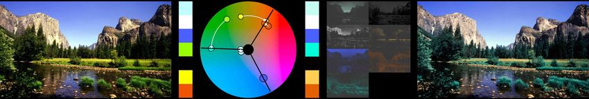
:2 •      Jianchao Tan, Jose Echevarria, and Yotam Gingold

                                                                                   In summary, this papers makes the following contributions:
                                                                                     • A new palette-based color harmonization framework, general
                                                                                       enough to model classical harmonic relationships, new color
                                                                                       composition operations, and a compact structure for other
                                                                                       color-aware applications, also applicable to video.
                                                                                     • An extremely efficient, geometric approach for decomposing
                                                                                       an image into spatially coherent additive mixing layers by
                                                                                       analyzing the geometry of an image in RGBXY-space. Its per-
                                                                                       formance is virtually independent from the size of the image
                                                                                       or palette. Our decomposition can be re-computed instanta-
                                                                                       neously for a new RGB palette, allowing designers to edit the
                                                                                       decomposition in real-time.
                                                                                     • Three large-scale, wide-ranging perceptual studies on the
                                                                                       perception of harmonic colors and our algorithm.
Fig. 2. Comparison between the sector-based hue harmonic templates
                                                                               We demonstrate other applications like color transfer, greatly sim-
from [Tokumaru et al. 2002] (shaded in grey), and our new axis-based ones.
We use two different types of axes: the dashed ones attract colors towards     plified by our framework.
them; the solid ones define sectors between them, so colors inside remain in
the same position, but colors outside are attracted towards them. We found     2     RELATED WORK
this distinction helps handling templates like analogous properly. Note that   There are many works related with our contributions and their
our templates derived from [Itten 1970] separate Y type into single split      applications. In the following we cover the most relevant ones.
and triad, and the same for X type. These templates are popular among
creatives, but they are also in agreement with the definitions of similarity   2.1    Color Harmonization
and ambiguity by Moon and Spencer [1944]. Although we don’t use it in
our results, our approach can also describe hybrid templates like L type.      Many existing works have applied different concepts from tradi-
Each template can be modeled by a single global rotation α 1 , although some   tional color theory for artists to improve the color composition of
of them have a secondary degree of freedom α 2 that enforces symmetry.         digital images. In their seminal paper, Cohen-Or et al. [2006] use
In this paper we focus on monochrome, complementary, single split, triad,      hue histograms and harmonic templates defined as sectors of hue-
double split, square and analogous.                                            saturation in HSV color space [Tokumaru et al. 2002], to model and
                                                                               manipulate color relationships. They fit a template (optimal or arbi-
                                                                               trary) over the image histogram, so they can shift hues accordingly
3D axes that capture color structure in a meaningful and compact               to harmonize colors or composites from several sources. Additional
way. This is useful for various color-aware tasks. We demonstrate              processing is needed to ensure spatial smoothness. Several people
applications to color harmonization and color transfer. Instead of             have built on top of this work, extending or improving parts of their
using the sector-based templates from Matsuda [Tokumaru et al.                 proposed framework. Sawant and Mitra [2008] extended it to video,
2002] (appropriate for hue histograms) we derive our harmonic tem-             focusing on temporal coherence between successive frames. Im-
plates from classical color theory [Birren and Cleland 1969; Itten             provements to the original fitting have been proposed based on the
1970] (see Figures 2 and 14). We also propose new color operations             number of pixels for each HSV value [Huo and Tan 2009], the visual
using this axes-based representation. Our proposed framework can               saliency [Baveye et al. 2013], the extension and visual weight of
be used by other palette-based systems and workflows, either for               each color. [Baveye et al. 2013], or geodesic distances [Li et al. 2015].
palette improvement or image editing.                                          Tang et al. [2010] improves some artifacts during the recoloring of
   At the core of our and other recent approaches [Aksoy et al. 2017;          [Cohen-Or et al. 2006]. Chamaret et al. [2014] defines and visualizes
Chang et al. 2015; Tan et al. 2016; Zhang et al. 2017] to image edit-          a per-pixel harmony measure to guide interactive user edits.
ing, images are decomposed into a palette and associated per-pixel                Instead of using hue histograms from images, our framework is
compositing or mixing parameters. We propose a new, extremely                  built on top of color palettes, independently of their source. Given
efficient yet simple and robust algorithm to do so. Our approach               the higher level of abstraction of palettes, we simplify harmonic
is inspired by the geometric palette extraction technique of Tan et            templates to arrangements of axes in chroma-hue space (from LCh),
al. [2016]. We consider the geometry of 5D RGBXY-space, which                  interpreted and derived directly from classical color theory [Birren
captures color as well as spatial relationships and eliminates numeri-         and Cleland 1969; Itten 1970]. This more general and simpler rep-
cal optimization. After an initial palette is extracted (given an RMSE         resentation makes for more intuitive metrics, easier to solve, that
reconstruction threshold), the user can edit the palette and obtain            enable a wider range of applications. When working with images,
new decompositions instantaneously. Our algorithm’s performance                this approach fits perfectly with our proposed palette extraction
is extremely efficient even for very high resolution images (≥ 100             and image decomposition for very efficient and robust image re-
megapixels)—20x faster than the state-of-the-art [Aksoy et al. 2017].          coloring. Related to our approach, Mellado et al. [2017] is also able
Working code is provided in Section 3. Our algorithm is a key con-             to pose harmonization as a set of constrains within their general
tribution which enables our approach and many other applications               constrained optimization framework. Our new templates, posed in
proposed in the literature.                                                    LCh space, could be added as additional constraints.

, Vol. 1, No. 1, Article . Publication date: June 2018.                                                   Submission ID: ***. 2018-06-22 00:18. Page 2 of 1–17.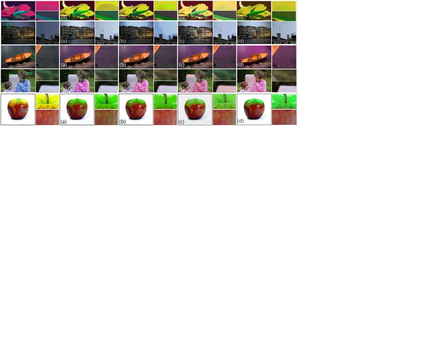
Palette-based image decomposition, harmonization, and color transfer • :3

   Finally, there is a different definition for harmony in composited          color themes as hue histograms in HSV space. Wang et al. [2010]
images, in terms of contrast, texture, noise or blur. Works dealing            solve an optimization that simultaneously considers a desired color
with it [Sunkavalli et al. 2010; Tsai et al. 2017] focus on a completely       theme, texture-color relationships as well as automatic or user-
different set of goals and challenges than the work discussed above.           specified color constraints. Phan et al. [2017] explored the order
                                                                               of colors within palettes to establish correspondences and enable
2.2    Palette Extraction and Image Decomposition                              interpolation. Nguyen et al. [2017] find a group color theme from
                                                                               multiple palettes from multiple images using a modified k-means
Palette Extraction A straightforward approach consists of using                clustering method, and use it to recolor all the images in a consis-
a k-means method to cluster the existing colors in an image, in                tent way. Han et al. [2017; 2013] compute a distance metric between
RGB space [Chang et al. 2015; Phan et al. 2017; Zhang et al. 2017].            palettes in the color mood space, and then sort and match colors from
A different approach consists of computing and simplifying the                 palettes according to their brightness. Munshi et al. [2015] match
convex hull enclosing all the color samples [Tan et al. 2016], which           colors between palettes according to their distance in Lab space.
provides more general palettes that better represent the existing              Based on our harmonic templates, palettes, and the LCh color space;
color gamut of the image. A similar observation was made in the                we propose several intuitive metrics for color transfer that take
domain of hyperspectral image unmixing [Craig 1994]. (With hy-                 into account human perception for goals like colorfulness, preser-
perspectral images, palette sizes are smaller than the number of               vation of original colors, or harmonic composition. The final image
channels, so the problem is one of fitting a minimum-volume sim-               recoloring is performed using our layer decomposition.
plex around the colors. The vertices of a high-dimensional simplex
become a convex hull when the data is projected to lower dimen-                3     PALETTE EXTRACTION AND IMAGE
sions.) Morse et al. [2007] work in HSL space, using a histogram to                  DECOMPOSITION
find the dominant hues, then to find shades and tints within them.
                                                                               A good palette for image editing is one that closely captures the
Human perception has also been taken into account in other works,
                                                                               underlying colors the image was made with (or could have been
training regression models on crowd-sourced datasets. [Lin and
                                                                               made with), even if those colors do not appear in their purest form
Hanrahan 2013; O’Donovan et al. 2011]. Some physically-based ap-
                                                                               in the image itself. Tan et al. [2016] observed that the color distribu-
proaches try to extract wavelength-dependent parameters to model
                                                                               tions from paintings and natural images take on a convex shape in
the original pigments used paintings. [Aharoni-Mack et al. 2017;
                                                                               RGB space. As a result, they proposed to compute the convex hull
Tan et al. 2017]. Our work builds on top of Tan et al. [2016], adding
                                                                               of the pixel colors. The convex hull tightly wraps the observed col-
a fixed reconstruction error threshold for automatic extraction of
                                                                               ors. Its vertex colors can be blended with convex weights (positive
palettes of optimal size, as described in Section 3.1.
                                                                               and summing to one) to obtain any color in the image. The convex
Image Decomposition For recoloring applications, it is also crit-              hull may be overly complex, so they propose an iterative simplifica-
 ical to find a mapping between the extracted color palette and the            tion scheme to a user-desired palette size. After simplification, the
 image pixels. Recent work is able to decompose the input image into           vertices become a palette that represents the colors in the image.
 separate layers according to a palette. Tan et al. [2016] extract a set of       We extend Tan et al. [2016]’s work in two ways. First, we propose
 ordered translucent RGBA layers, based on a optimization over the             a simple, geometric layer decomposition method that is orders of
 standard alpha blending model. Order-independent decompositions               magnitude more efficient than the state-of-the-art. Working code
 can be achieved using additive color mixing models [Aksoy et al.              for our entire decomposition algorithm can be written in under 50
 2017; Lin et al. 2017a; Zhang et al. 2017]. For the physically-based          lines (Figure 4). Second, we propose a simple scheme for automatic
 palette extraction methods mentioned previously [Aharoni-Mack                 palette size selection.
 et al. 2017; Tan et al. 2017], layers correspond to the extracted multi-
 spectral pigments. We prefer a full decomposition to a (palette-based)        3.1    Palette Extraction
 edit transfer approach like Chang et al. [2015]’s. With a full decom-         In Tan et al. [2016], the convex hull of all pixel colors is computed
 position, edits are trivial to apply and spatial edits become possible        and then simplified to a user-chosen palette size. To summarize their
 (though we do not explore spatial edits in this work). We present             approach, the convex hull is simplified greedily as a sequence of
 a new, efficient method for layer decomposition, based on the ad-             constrained edge collapses [Garland and Heckbert 1997]. An edge
 ditive color mixing model (Section 3.2). Our approach leverages               is collapsed to a point constrained to strictly add volume [Sander
 5D RGBXY-space geometry to enforce spatial smoothness on the                  et al. 2000] while minimizing the distance to its incident faces. The
 layers. This geometric approach is significantly more efficient than          edge whose collapse adds the least overall volume is chosen next,
 previous approaches in the literature, easily handling images up to           greedily. After each edge is collapsed, the convex hull is recomputed,
 100 megapixels in size.                                                       since the new vertex could indirectly cause other vertices to become
                                                                               concave (and therefore redundant). Finally, simplification may result
2.3    Color Transfer                                                          in out-of-gamut colors, or points that lie outside the RGB cube. As
We also explore color transfer as an application of our work. Color            a final step, Tan et al. [2016] project all such points to the closest
transfer is a vast field with contributions from the vision and graph-         point on the RGB cube. This is the source of reconstruction error in
ics communities. As such, we describe only the most closely related            their approach; some pixels now lie outside the simplified convex
work to our approach. Hou et al. [2007] conceptualize and apply                hull and cannot be reconstructed.

Submission ID: ***. 2018-06-22 00:18. Page 3 of 1–17.                                                      , Vol. 1, No. 1, Article . Publication date: June 2018.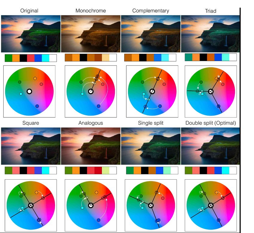
:4 •      Jianchao Tan, Jose Echevarria, and Yotam Gingold

   We improve upon this procedure with the observation that the
reconstruction error can be measured geometrically, even before
layer decomposition, as the RMSE of every pixel’s distance to the
simplified convex hull. (Inside pixels naturally have distance 0.)
Therefore, we propose a simple automatic palette size selection
based on a user-provided RMSE reconstruction error tolerance ( 255   2
in our experiments). For efficiency, we divide RGB-space into 32 ×
32 × 32 bins (a total of 215 bins). We measure the distance from each
non-empty bin to the simplified convex hull, weighted by the bin
count. We start measuring the reconstruction error once the number
of vertices has been simplified to 10. By doing this, we are able to
obtain palettes with an optimal number of colors automatically. This
removes the need for the user to choose the palette size manually,
leading to better layer decompositions.
   (If non-constant palette colors were acceptable, instead of clipping
one could cast a ray from each pixel towards the out-of-gamut vertex;
the intersection of the ray with the RGB cube would be the palette
color for that pixel. There would be zero reconstruction error. The
stopping criteria could be the non-uniformity of a palette color,
measured by the area of the RGB cube surface intersected with the
simplified convex hull itself.)

3.2     Image decomposition via RGBXY convex hull
                                                                          Fig. 3. Visualization of the two convex hulls. Left: the simplified RGB convex
From their extracted palettes, Tan et al. [2016] solved a non-linear
                                                                          hull is the basis for the methods in Tan et al. [2016], capturing the colors of
optimization problem to decompose an image into a set of ordered,         an image but not their spatial relationships. Right: Our 5D RGBXY convex
translucent RGBA layers suitable for the standard “over” composit-        hull captures color and spatial relationship at the same time. We visualize
ing operation. While this decomposition is widely applicable (owing       its vertices as small circles; its 5D simplices are difficult to visualize. Our
to the ubiquity of “over” compositing), the optimization is quite         approach splits image decomposition into a two-level geometric problem.
lengthy due to the recursive nature of the compositing operation,         The first level are the RGBXY convex hull vertices that mix to produce
which manifests as a polynomial whose degree is the palette size.         any pixel in the image. The second level are the simplified RGB convex
Others have instead opted for additive mixing layers [Aksoy et al.        hull vertices, which serve as the palette RGB colors. Since the RGBXY
2017; Lin et al. 2017a; Zhang et al. 2017] due to their simplicity. A     convex hull vertices lie inside the RGB convex hull, we find mixing weights
pixel’s color is a weighted sum of the palette colors.                    that control the color of the RGBXY vertices. The two levels combined
                                                                          allow instant recoloring of the whole image. The top right image shows the
   In this work, we adopt linear mixing layers as well. We provide a
                                                                          locations of the RGBXY vertices in image space. The bottom row shows the
fast and simple, yet spatially coherent, geometric construction.          geometric relationships between the 3D and 5D convex hull vertices, and
   Any point p inside a simplex (a triangle in 3D, a tetrahedron          how the simplified RGB convex hull captures the same color palette for both
in 3D, etc.) has a unique set of barycentric coordinates, or convex       algorithms.
additive mixing weights such that p = i w i ci , where the mixing
                                          Í
weights w i are positive and sum to one, and ci are the vertices of
the simplex. In our setting, the simplified convex hull is typically         This is the approach taken by Tan et al. [2016] for their as-sparse-
not a simplex, because the palette has more than 4 colors. There          as-possible (ASAP) technique to extract layers. Because Tan et al.
still exist convex weights w i for arbitrary polyhedron, known as         [2016] considered recursive over compositing, users provided a
generalized barycentric coordinates [Floater 2015], but they are          layer or vertex order; they tessellated the simplified convex hull
typically non-unique. A straightforward technique to find general-        by connecting all its (triangular) faces to the first vertex, which
ized barycentric coordinates is to first compute a tessellation of the    corresponds to the background color. This simple star tessellation is
polyhedron (in our case, the simplified convex hull) into a collec-       valid for any convex polyhedron. In the additive mixing scenario,
tion of non-overlapping simplices (tetrahedra in 3D). For example,        no order is provided; we discuss the choice of tessellation below.
the Delaunay generalized barycentric coordinates for a point can be       Because the weights are assigned purely based on the pixel’s colors,
computed by performing a Delaunay tessellation of the polyhedron.         however, this approach predictably suffers from spatial coherence
The barycentric coordinates of whichever simplex the point falls          artifacts (Figure 7). The colors of spatially neighboring pixels may
inside of are the generalized barycentric coordinates. For a 3D point     belong to different tetrahedra. As a result, ASAP layers produce
in general position in the interior, the mixing weights will have         speckling artifacts during operations like recoloring (Figure 7).
at most 4 non-zero weights, which corresponds to the number of
vertices of a tetrahedron.                                                Spatial Coherence To provide spatial coherence, our key insight
                                                                           is to extend this approach to 5D RGBXY-space, where XY are the

, Vol. 1, No. 1, Article . Publication date: June 2018.                                                 Submission ID: ***. 2018-06-22 00:18. Page 4 of 1–17.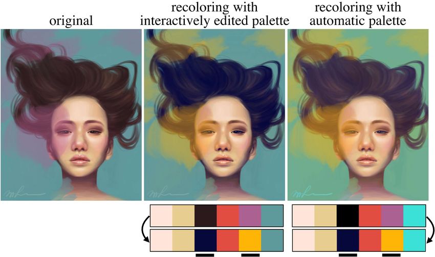
Palette-based image decomposition, harmonization, and color transfer • :5

                                                                                  from numpy import *¬
coordinates of a pixel in image space, so that spatial relationship               from scipy.spatial import ConvexHull, Delaunay¬
                                                                                  from scipy.sparse import coo_matrix¬
are considered along with color in a unified way (Figure 3). We first             ¬
the compute convex hull of the image in RGBXY-space. We then                      def RGBXY_weights( RGB_palette, RGBXY_data ):¬
                                                                                      RGBXY_hull_vertices = RGBXY_data[ ConvexHull( RGBXY_data ).vertices ]¬
compute Delaunay generalized barycentric coordinates (weights)                        W_RGBXY = Delaunay_coordinates( RGBXY_hull_vertices, RGBXY_data )¬
                                                                                      # Optional: Project outside RGBXY_hull_vertices[:,:3] onto RGB_palette convex hull.¬
for every pixel in the image in terms of the 5D convex hull. Pixels                   W_RGB = Star_coordinates( RGB_palette, RGBXY_hull_vertices[:,:3] )¬
                                                                                      return W_RGBXY.dot( W_RGB )¬
that have similar colors or are spatially adjacent will end up with               ¬
similar weights, meaning that our layers will be smooth both in RGB               def Star_coordinates( vertices, data ):¬
                                                                                      ## Find the star vertex¬
and XY-space. These mixing weights form an Q × N matrix WRGBXY ,                      star = argmin( linalg.norm( vertices, axis=1 ) )¬

where N is the number of image pixels and Q is the number of                          ## Make a mesh for the palette¬
                                                                                      hull = ConvexHull( vertices )¬
RGBXY convex hull vertices. We also compute WRGB , Delaunay                           ## Star tessellate the faces of the convex hull¬
                                                                                      simplices = [ [star] + list(face) for face in hull.simplices if star not in face ]¬
barycentric coordinates (weights) for the RGBXY convex hull ver-                      barycoords = -1*ones( ( data.shape[0], len(vertices) ) )¬
                                                                                      ## Barycentric coordinates for the data in each simplex¬
tices in the 3D simplified convex hull. We use the RGB portion of                     for s in simplices:¬
each RGBXY convex hull vertex, which always lies inside the RGB                           s0 = vertices[s[:1]]¬
                                                                                          b = linalg.solve( (vertices[s[1:]]-s0).T, (data-s0).T ).T¬
convex hull. Due to the aforementioned out-of-gamut projection                            b = append( 1-b.sum(axis=1)[:,None], b, axis=1 )¬
                                                                                          ## Update barycoords whenever the data is inside the current simplex.¬
step when computing the simplified RGB convex hull, however, an                           mask = (b>=0).all(axis=1)¬
RGBXY convex hull vertex may occasionally fall outside it. We set                         barycoords[mask] = 0.¬
                                                                                          barycoords[ix_(mask,s)] = b[mask]¬
its weights to those of the closest point on the 3D simplified convex                 return barycoords¬
                                                                                  ¬
hull. WRGB is a P × Q matrix, where P is the number of vertices of                def Delaunay_coordinates( vertices, data ): # Adapted from Gareth Rees¬
the simplified RGB convex hull (the palette colors).                                  # Compute Delaunay tessellation.¬
                                                                                      tri = Delaunay( vertices )¬
   The final weights for the image are obtained via matrix multipli-                  # Find the tetrahedron containing each target (or -1 if not found).¬
                                                                                      simplices = tri.find_simplex(data, tol=1e-6)¬
cation: W = WRGBWRGBXY , which is a P × N matrix that assigns                         assert (simplices != -1).all() # data contains outside vertices.¬
                                                                                      # Affine transformation for simplex containing each datum.¬
each pixel weights solely in terms of the simplified RGB convex                       X = tri.transform[simplices, :data.shape[1]]¬
hull. These weights are smooth both in color and image space. To                      # Offset of each datum from the origin of its simplex.¬
                                                                                      Y = data - tri.transform[simplices, data.shape[1]]¬
decompose an image with a different RGB-palette, one only needs                       # Compute the barycentric coordinates of each datum in its simplex.¬

to recompute WRGB and then perform matrix multiplication. Com-                        b = einsum( '...jk,...k->...j', X, Y )¬
                                                                                      barycoords = c_[b,1-b.sum(axis=1)]¬
puting WRGB is extremely efficient, since it depends only on the                      # Return the weights as a sparse matrix.¬
                                                                                      rows = repeat(arange(len(data)).reshape((-1,1)), len(tri.simplices[0]), 1).ravel()¬
palette size and the number of RGBXY convex hull vertices. It is                      cols = tri.simplices[simplices].ravel()¬
                                                                                      vals = barycoords.ravel()¬
independent of the image size and allows users to experiment with                     return coo_matrix( (vals,(rows,cols)), shape=(len(data),len(vertices)) ).tocsr()
image decompositions based on interactive palette editing (Figure 10
and the supplemental materials).                                                  Fig. 4. Python code for our RGBXY additive mixing layer decomposition
                                                                                  (48 lines).
Tessellation At first glance, any tessellation of 3D RGB-space has
 approximately the same ℓ0 weight sparsity (4 non-zeros). In practice,
 the “line of greys” between black and white is critically important.                We also experimented with a variety of strategies to choose the
Any pixel near the line of greys can be expressed as the weighted                 tessellation such that the resulting layer decomposition is as sparse
 combination of vertices in a number of ways (e.g. any tessellation). It          as possible: RANSAC line fitting and PCA on the RGB point cloud
 is perceptually important that the line of greys be 2-sparse in terms            and finding the longest edge. We evaluated the decompositions
 of an approximately black and white color, and that nearby colors                with several sparsity metrics ([Aksoy et al. 2017; Levin et al. 2008;
 be nearly 2-sparse. If not, then grey pixels would be represented as             Tan et al. 2016], as well as the fraction of pixels with transparency
 mixtures of complementary colors; any change to the palette that                 above a threshold). Ultimately, tinting was more perceptually salient
 didn’t preserve the complementarity relationships would turn grey                than changes in sparsity, and our proposed tessellation algorithm is
 pixels colorful (Figure 7). This tinting is perceptually prominent and           simpler and robust.
 undesirable.1 .
    To make the line of greys 2-sparse in this way, the tessellation              3.3   Evaluation
 should ensure that an edge is created between the darkest and
 lightest color in the palette. Such an edge is typically among the              Quality The primary means to assess the quality of layers is to
 longest possible edges through the interior of the polyhedron, as               apply them for some purpose, such as recoloring, and then iden-
 the luminance in an image often varies more than chroma × hue.                  tify artifacts, such as noise, discontinuities, or surprisingly affected
As a result, the Delaunay tessellation frequently excludes the most              regions. Figure 6 compares recolorings created with our layers to
 desirable edge through the line of greys. We propose to use a star              those from Aksoy et al. [2017], Tan et al. [2016], and Chang et al.
 tessellation. If either a black or white palette color is chosen as the         [2015]. Our approach generates recolorings without discontinuities
 star vertex, it will form an edge with the other. We choose the darkest         (the sky in (b), second row), undesirable changes (the top of the
 color in the palette as the star vertex. This strategy is simple and            chair in (c), third row), or noise.
 robust and extends naturally to premultiplied alpha RGBA images.                   We have no explicit guarantees about the sparsity of our weights.
1 Forpathalogical images containing continuous gradients between complementary   WRGB is as sparse as possible to reconstruct 3D colors (4 non-zeros).
colors, this tinting behavior would perhaps be desired.                          WRGBXY has 6 non-zeros among the (typically) 2000–5000 RGBXY

Submission ID: ***. 2018-06-22 00:18. Page 5 of 1–17.                                                               , Vol. 1, No. 1, Article . Publication date: June 2018.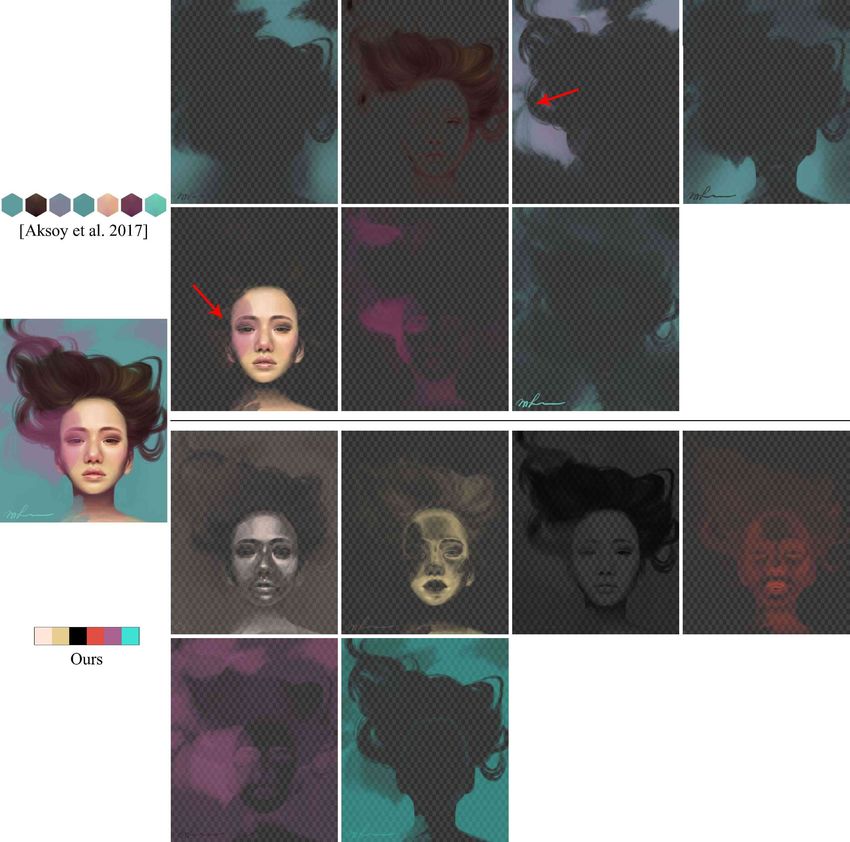
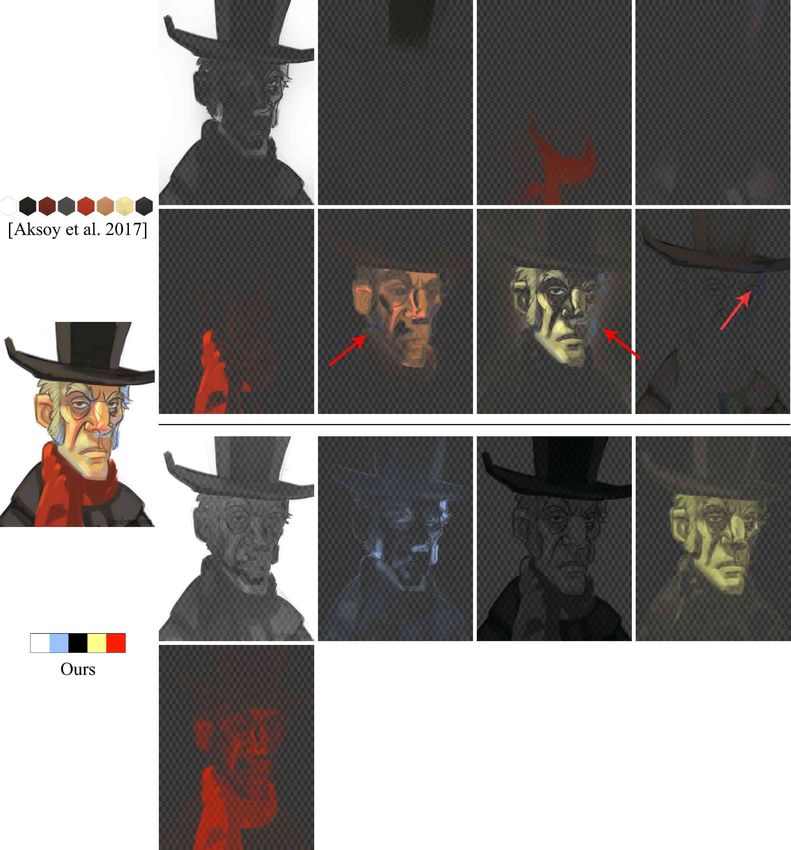
:6 •      Jianchao Tan, Jose Echevarria, and Yotam Gingold

Fig. 5. A comparison between our proposed RGBXY image decomposition and that of Aksoy et al. [2017]. Aksoy et al. [2017] creates an overabundance of
layers (two red layers above) and does not extract the blueish tint, which appears primarily in mixture. Our RGBXY technique identifies mixed colors is able to
separate the translucent purple haze in front of the girl’s face. Additionally, our GUI allows editing the palette to modify layers in real time. This allows users
to further improve the decomposition, as shown in Figure 10 and the supplemental materials.

Fig. 6. To evaluate our RGBXY decomposition algorithm, we compare our layers with previous approaches in a recoloring application. From left to right: (a)
Aksoy et al. [2017], (b) Tan et al. [2016], (c) Chang et al. [2015] and (d) our approach. Our recoloring quality is similar to the state of the art, but our method is
orders of magnitude faster and allows interactive layer decomposition while editing palettes.

, Vol. 1, No. 1, Article . Publication date: June 2018.                                                              Submission ID: ***. 2018-06-22 00:18. Page 6 of 1–17.
Palette-based image decomposition, harmonization, and color transfer • :7

                                                                                   convex hull vertices, which is also as sparse as possible to recover
                                                                                   a point in RGBXY-space. The sparsity of the product of the two
                                                                                   matrices depends on which 3D tetrahedra the 6 RGBXY convex
                                                                                   hull vertices fall into. Nevertheless, it can be seen that our results’
                                                                                   sparsity is almost as good as Tan et al. [2016].
                                                                                      Figure 5 shows a direct comparison between our additive mixing
                                                                                   layers and those of Aksoy et al. [2017] for direct inspection. In con-
                                                                                   trast with our approach, Aksoy et al. [2017]’s approach has trouble
                                                                                   separating colors that appear primarily in mixture. As a result, Ak-
                                                                                   soy et al. [2017]’s approach sometimes creates an overabundance of
                                                                                   layers, which makes recoloring tedious, since multiple layers must
                                                                                   be edited.
                                                                                      Our decomposition algorithm is able to reproduce input images
                                                                                   virtually indistinguishably from the originals. For the 100 images in
                                                                                   Figure 8, our RGBXY method’s RGB-space RMSE is typically 2 − −3.
                                                                                   Aksoy et al. [2017]’s algorithm reconstruct images with zero error,
                                                                                   since their palettes are color distributions rather than fixed colors.
                                                                                      We evaluate our RGB tessellation in Figure 7. In this experiment,
                                                                                   we generate a random recoloring by permuting the colors in the
Fig. 7. Comparing tessellation strategies for color palettes in RGB-space. The     palette. The RGB-space star triangulation approach is akin to Tan
Delaunay tessellation column computes Delaunay barycentric coordinates             et al. [2016]’s ASAP approach with the black color chosen to be
for the color palette. This tessellation often avoids creating the perceptually    the first layer. The lack of spacial smoothness is apparent in be-
important line of greys, leading to tinting artifacts. These are avoided with      tween the RGB-only decompositions in the top-row and the RGBXY
a star tessellation emanating from the vertex closest to black. Computing          decompositions in the bottom row. The decompositions using the
weights in RGB-space alone leads to spatial smoothness artifacts. Our two-         Delaunay generalized barycentric coordinates (left column) result
stage RGBXY decomposition provides color and spatial smoothness. To
                                                                                   in undesirable tinting for colors near the line of grey. Additional
interrogate the quality of layer decompositions, we randomly permute the
palette, revealing problems in computed weights. See the supplemental
                                                                                   examples can be found in the supplemental materials.
materials for additional examples.                                                    Throughout the remainder of the paper, all our results rely on
                                                                                   our proposed layer decomposition.

                                                                                  Speed In Figure 8, we compare the running time of additive mix-
                                                                                   ing layer decomposition techniques. We ran our proposed RGBXY
                                                                                   approach on 100 images under 6 megapixels with an average palette
                                                                                   size of 6.95 and median palette size of 7. Computation time for
                                                                                   our approaches includes palette selection (RGB convex hull sim-
                                                                                   plification). Because of its scalability, we also ran our proposed
                                                                                   RGBXY approach on an additional 70 large images between 6 and 12
                                                                                   megapixels, and an additional 6 extremely large images containing
                                                                                  100 megapixels (not shown in the plot). The 100 megapixel images
                                                                                   took on average 12.6 minutes to compute. Peak memory usage was
                                                                                  15 GB. For further improvement, our approach could be parallelized
                                                                                   by dividing the image into tiles, since the convex hull of a set of
                                                                                   convex hulls is the same as the convex hull of the underlying data.
                                                                                  A working implementation of the RGBXY decomposition method
                                                                                   can be found in Figure 4 (48 lines of code). The “Layer Updating”
Fig. 8. Running time comparison between four additive mixing image de-             performance is nearly instantaneous, taking a few milliseconds to,
composition algorithms. We evaluated our RGBXY algorithm on 170 images             for 10 MP images, a few tens of milliseconds to re-compute the layer
up to 12 megapixels and an additional six 100 megapixel images (not shown;         decomposition given a new palette.
average running time 12.6 minutes). Our algorithm’s performance is orders
                                                                                      Our running times were generated on a 2015 13” MacBook Pro
of magnitude faster and scales extremely well with image size. The number
                                                                                  with a 2.9 GHz Intel Core i5-5257U CPU and 16 GB of RAM. Our layer
of RGBXY convex hull vertices has a greater effect on performance than
image size. Re-computing our layer decomposition with an updated palette           decomposition approach was written in non-parallelized Python
is nearly instantaneous (a few to tens of milliseconds).                           using NumPy/SciPy and their wrapper for the QHull convex hull
                                                                                   and Delaunay tessellation library [Barber et al. 1996]. Our layer
                                                                                   updating was written in OpenCL.
                                                                                      Aksoy et al. [2017]’s performance is the fastest previous work
                                                                                   known to us. The performance data for Aksoy et al.’s algorithm is

Submission ID: ***. 2018-06-22 00:18. Page 7 of 1–17.                                                          , Vol. 1, No. 1, Article . Publication date: June 2018.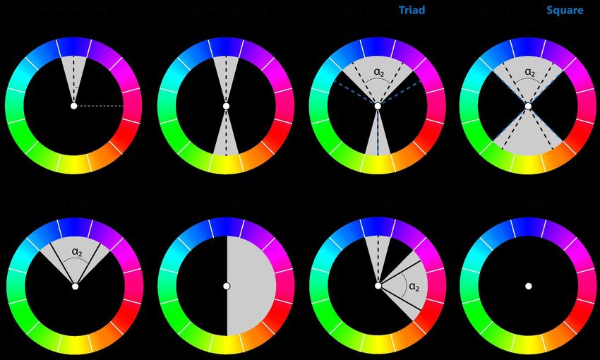
:8 •      Jianchao Tan, Jose Echevarria, and Yotam Gingold

as reported in their paper and appears to scale linearly in the pixel
size. Their algorithm was implemented in parallelized C++. Aksoy
et al. [2017] reported that their approach took 4 hours and 25 GB of
memory to decompose a 100 megapixel image. Zhang et al. [2017]’s
sole performance data point is also as reported in their paper.
   We also compare our approach to a variant of Tan et al. [2016]’s
optimization. We modified their reconstruction term to the simpler,
quadratic one that matches our additive mixing layer decomposition
scenario. With that modification, all energy terms become quadratic.
However, because the sparsity term is not positive definite, it is not
a straightforward Quadratic Programming problem; we minimize
it with L-BFGS-B and increased the solver’s default termination
thresholds since RGB colors have low precision (gradient and func-
tion tolerance 10−4 ). This approach was also written in Python using
NumPy/SciPy. The performance of the modified Tan et al. [2016]
is somewhat unpredictable, perhaps owing to the varying palette            Fig. 9. Our GUI for interactively editing palettes. See the text for details.
sizes.
   The fast performance of our approach is due to the fact that the
number of RGBXY convex hull vertices Q is virtually independent of
the image size and entirely independent of the palette size. Finding
the simplex that contains a point is extremely efficient (a matrix
multiply followed by a sign check) and scales well. Our algorithm’s
performance is more correlated with the number of RGBXY convex
hull vertices and tessellated simplices. This explains the three red
dots somewhat above the others in the performance plot.
   In contrast, optimization-based approaches typically have param-
eters to tune, such as the balance between terms in the objective
function, iteration step size, and termination parameters.

Interactive Layer Decompositions To take advantage of our ex-
 tremely fast layer decomposition, we implemented an HTML/JavaScript
 GUI for viewing and interacting with layer decompositions (Fig-
 ure 9). An editing session begins when a user loads an image and
 precomputes RGBXY weights. Users can then begin with a generic            Fig. 10. Our GUI allows users edit palettes and see the resulting layer de-
 tetrahedron or with an automatically chosen palette, optionally with      composition in real-time. Videos of live palette editing can be found in
 a prescribed number of layers. Users can alter the palette colors in      the supplemental materials. In this example, the automatic palette (right)
 3D RGB-space (lower-left) or activate a traditional color picker by       becomes sparser as a result of interactive editing. The user edits the auto-
                                                                           matically generated palette to ensure that the background and hair colors
 clicking on a layer (the turquoise layer as shown). As users drag the
                                                                           are directly represented. As a result, editing the purple haze and hair no
 palette colors, the layer decomposition updates live. (Although our
                                                                           longer affects the background color.
 layer updating algorithm computes at an extremely high frame rate,
 the bulk of the time in our GUI is spent transferring the data to the
 browser via a WebSocket.) Users can also add and then manipulate
 additional colors. See Figure 10 for a result created with our GUI;
 see the supplemental materials for screen recordings of this and          4.1   Template fitting
 other examples.                                                           Figure 2 shows our new axis-based templates compared to the sector-
                                                                           based ones from Tokumaru et al. [2002]. For our results in this paper
                                                                           we use seven templates Tm , m = 1...7. A template is defined by
4    COLOR HARMONIZATION                                                     j
                                                                           Tm (α), where j is the index of each axis (the total number of axes
In the following we describe our palette-based approach to color           varies between templates), and α is an angle of rotation in hue.
harmonization and color composition. Our work is inspired by the           While our templates are valid in any circular (or cylindrical) color
same concepts and goals as related previous work [Cohen-Or et al.          space (e.g. HSV), we apply them in LCh-space (Lightness, Chroma,
2006]. However, we also aim for a simpler and more compact rep-            and hue) to match human perception.
resentation that can express additional operations and be applied              Given an image I and its extracted color palette P, we seek to
directly to palettes. First, we explain how we fit and enforce classical   find the Tm (α) that is closest to the colors in P in the Ch plane. For
harmonic templates. Next, we describe how our framework can be             that, we find the closest axis to each color, and solve for the global
used for other color composition operations.                               rotation and additional angles that define the template. We define

, Vol. 1, No. 1, Article . Publication date: June 2018.                                                 Submission ID: ***. 2018-06-22 00:18. Page 8 of 1–17.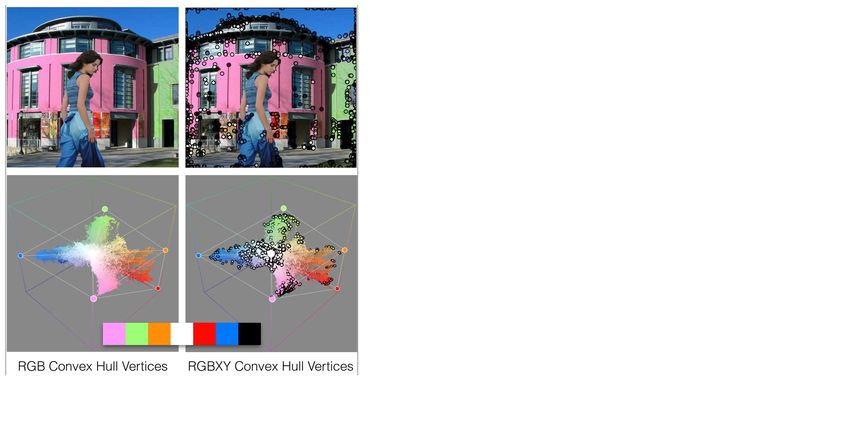
Palette-based image decomposition, harmonization, and color transfer • :9
Fig. 12. Results from enforcing a given template Tm (α ∗ ) with varying de-
grees of strength β . Bottom left shows the consistent palette interpolation
across β = [0, 1.5]. Even beyond β = 1 (full harmonization), results remain
predictable.
allow an additional degree of freedom (angle between axes), which
we allow [−15, 15] degrees. In this case, αm ∗ = [α ∗ , α ∗ ]. With
m,1 m,2
αm,1 being the optimal global rotation, and αm,2
∗ ∗ the optimal angle
between axes. Given that palettes are typically small (less than 10
colors), our brute force search is very fast (less than a second).
Once a template is fit, we harmonize the input image by using
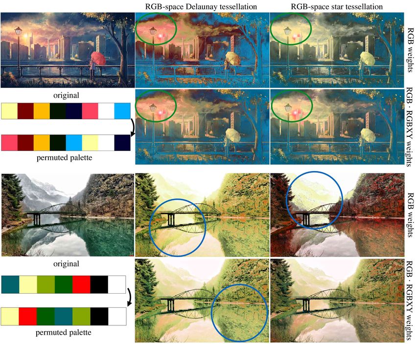
Fig. 11. Results of our harmonic templates fit to the an input image. We Tm (αm∗ ) to move the colors in P closer to the axis assignment that
can see how each of them is able to provide a balanced and pleasing look minimizes equation 1. We leverage the image decomposition to
when the harmonization is fully enforced. In an interactive application, the recolor the image. Because we use a spatially coherent image de-
user can control the strength of harmonization, which interpolates the hue composition, no additional work is needed to prevent discontinuous
rotation of each palette color. recoloring as in Cohen-Or et al. [2006]. Figure 11 shows different
harmonic templates enforced over the same input image. Additional
examples can be found in the supplementary material. Users can
the distance D between a palette P and a template Tm (α) as:
control the strength of harmonization via an interpolation param-
|P |
Õ
j∗ eter, where β = 0 leaves the palette unchanged and β = 1 fully
D(P,Tm (α)) = W (Pi ) · L(Pi ) · C(Pi ) · H (Pi ) − Tm (α) (1) rotates each palette color to lie on its matched axis (Figure 12). In
i=1 the LCh color space, this affects hue alone.
j
j ∗ = arg min H (Pi ) − Tm (α) Depending on the colors in P, some templates are a better fit than
j=1...#axes others as measured by Equation 1. We can determine the optimal
where j ∗ is the axis of template Tm (α) that is closest to palette template Tm ∗ automatically:
color Pi . |·| measures the difference in Hue angle. Note that for the ∗ ∗
Tm = arg min D(P,Tm (αm )) (3)
analogous template, any palette color inside that arc area will be Tm
zero distance to the template. W (Pi ) is the contribution of color Pi
to all the pixels in image, computed as the sum of all the weights for Depending on the palette size or its distribution, some axes may
layer i and normalized by the total number of pixels in the image. end up without any color assigned to them. We deem those cases
W (Pi ) promotes the template to be better aligned with the relevant not compliant with the intended balance of the harmonic template
colors of the image. When using color palettes that do not come and remove them from this automatic selection.
from images, W (Pi ) is the same for each color and can be discarded. Figure 13 shows the best fitting template for a set of images, and
The lightness L(Pi ) and chroma C(Pi ) of the color are also used as the fully harmonized result. More examples can be found in the
weights so that we measure the arc distance around the color wheel supplementary material. We compare our results with harmoniza-
(the angular change scaled by radius). The darker the color or the tions from previous works in Figure 17. While our result is clearly
less saturated, the smaller the perceived change per hue degree. different, it arguably produces a more balanced result. Cohen-Or
Since the search space is a finite range in 1D, we use a brute-force et al. [2006] demonstrated harmonization between different parts of
search to find the optimal global rotation angle αm∗ fitting a template an image using masks or harmonization of image composites. We
Tm (α) to a palette P: provide comparisons for this scenario in Figure 18.
∗
αm = arg min D(P,Tm (α)) (2) 4.2 Beyond hue
α Our compact representation using palettes and axis-based templates
Monochrome, complementary, triad and square templates have allows to formulate full 3D color harmonization operations easily.
only one degree of freedom, so we search the global rotation every
1 degree in [0, 360]. For analogous, single split and double split we LC harmonization
Submission ID: ***. 2018-06-22 00:18. Page 9 of 1–17. , Vol. 1, No. 1, Article . Publication date: June 2018.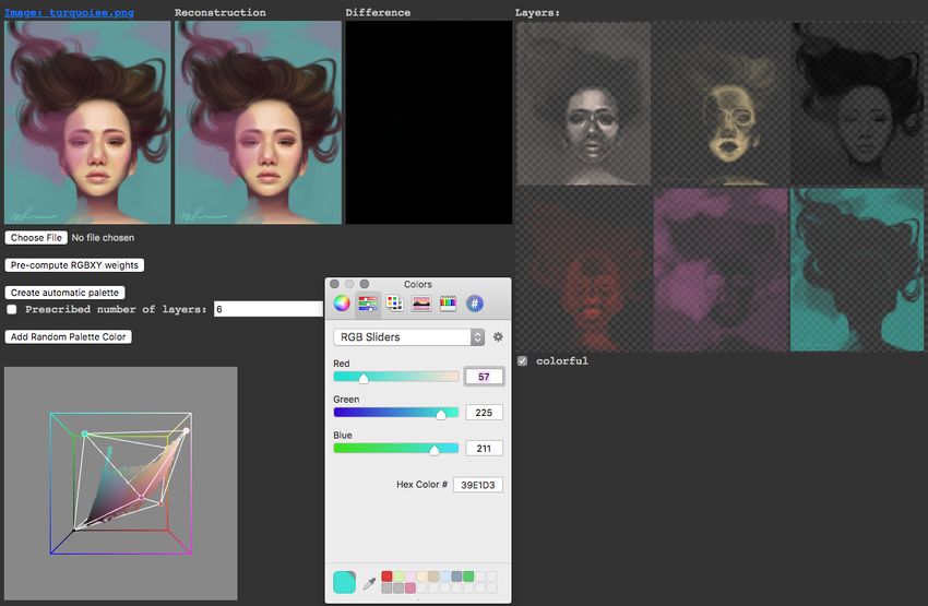
:10 •      Jianchao Tan, Jose Echevarria, and Yotam Gingold

Fig. 13. Examples of optimal templates for different images, and the fully
harmonized results they produce.

   Apart from hue, some authors have described harmony in terms              Fig. 14. Our LC templates derived from classical color theory. Template
of lightness and chroma as well [Birren and Cleland 1969; Moon               fitting solves for ϵn for each case. From left to right, top to bottom: LC 1
and Spencer 1944; Tokumaru et al. 2002]. While histogram-based               aligns colors vertically so hue and chroma remain constant, and places
approaches may be non-trivial to extend to these additional dimen-           them separated by uniform lightness steps. LC 2 enforces constant hue
sions, our approach generalizes to them easily. Figure 14 shows              and lightness, and does the uniform distribution for chroma. LC 3 and LC 4
our interpretation of the most typical LC templates defined in the           are alternative diagonal distributions that pivot around 0LC = {0, 0} and
literature. Analogous to our hue templates, we use W (Pi ) to find           1LC = {1, 0} respectively. LC 5 fits colors to a diagonal with an angle of
the optimal ϵn∗ for each template LCn , n = 1...6, and the best fitting      45◦ that displaces horizontally. LC 6 is the mirrored version of LC 5 . For
                                                                             complementary and multi-axis hue templates, LC 3 pivots around N LC =
template LCn∗ .
                                                                             {0.5, 0} for each axis. Additional optional constrains specified in [Birren
   Snapping colors to a template LCn requires finding the 2D line
                                                                             and Cleland 1969], enforce one of the colors to have a neutral lightness of
that fits best the LC distribution of the colors over a narrow hue band.     0.5. We implement this as a global offset to make the closest color to L = 0.5
To do that we minimize a weighted sum of all the perpendicular               snap into it (blue dotted line), as seen in template LC 1 . When P includes
distances from each color to the axis of LCn , weights are the same          pure white or black, we found leaving them out of the harmonization works
W (Pi ) from Subsection 4.1. Specifically:                                   best. Circles show original colors, stars indicate their harmonized location.
     • For LC 1 , the optimal position for the vertical axis after the
       optimization is ϵ1∗ = W (Pi ) ∗ C(Pi ).
                              Í
     • For LC 2 , the optimal horizontal axis is ϵ2∗ = W (Pi ) ∗ L(Pi ).
                                                      Í
     • For LC 3 and LC 4 , we look for the axis pivoting from 0LC =          hue templates. For multi-axis templates, specific arrangements are
       {0, 0} and 1LC = {1, 0}. We search for the axis rotation by           described by Munsell [Birren and Cleland 1969] for complementary
       brute force every 1◦ to find the optimal min(ϵ3∗ , ϵ4∗ )              schemes, in terms of visual balance between the two axes, pivoting
     • For LC 5 , the diagonal line equation is x − y − d = 0, where x       around a neutral point. We implement this idea by applying LC 3,4
       is C and y is L. Then optimal displacement ϵ5∗ = W (Pi ) ∗            pivoting around N LC = {0.5, 0} for each axis. This approach can
                                                             Í
       (C(Pi ) − L(Pi ))                                                     handle an arbitrary number of axis, although for palettes of optimal
     • For LC 6 , the line equation is x + y − d = 0. Then optimal           size, sometimes it is difficult to find more than one color per axis.
       displacement ϵ6∗ = W (Pi ) ∗ (C(Pi ) + L(Pi )).
                            Í
                                                                             Figure 15 shows examples of LC harmonization. It is worth men-
  For all templates, after line fitting we find the two extreme colors       tioning that while our hue harmonization is always able to produce
for the axis, and space the remaining ones evenly between those.             colorful results that preserve shading and contrast, harmonizing
  As can be seen, LCn are defined primarily for a single axis, and           lightness and chroma may produced unwanted loss of contrast when
so they are directly applicable to monochromatic and analogous               enforcing templates other than the optimal LCn∗ .

, Vol. 1, No. 1, Article . Publication date: June 2018.                                                   Submission ID: ***. 2018-06-22 00:18. Page 10 of 1–17.
Palette-based image decomposition, harmonization, and color transfer • :11
Fig. 15. LC harmonization examples. From top to bottom: Extracted palette
from input image. Palette hue harmonization for the monochromatic and
complementary (last column only) template. Palette LC harmonizations
as seen in Figure 14. Image hue harmonization. Image LC harmonization
applied on top of the previous hue harmonization. Changes from LC har-
monization are more apparent between the palettes, and more subtle on the
recolored images. This is expected because LC n∗ is applied to each image,
producing more subtle results. Fig. 16. Examples from the warm-cool contrast operator.
Color-based contrast As part of his seminal work on color com-
position for design, Itten [1970] described additional pleasing color
arrangements to create contrast. In contrast with sector-based tem-
plates, it is straightforward to model them with our axis-based repre-
sentation. Here is the exhaustive list of Itten’s additional contrasting
color arrangements and how they fit into our framework:
• Hue: Triad template aligned with the RGB primaries. No need
to solve for α ∗ .
• Light-dark: analogous or monochrome template, plus LC 1 .
• Complementary: same as complementary hue template.
Fig. 17. Comparison of harmonizations using the best fitting template from
• Simultaneous: complementary template, plus the axis with
different methods. Cohen-Or et al. [2006] fit a complementary (I type) tem-
the smaller overall W scales down its chroma proportionally plate in HSV space, producing unexpected changes in lightness for some
to β. colors. Mellado et al. [2017] formulated the same harmonic template us-
• Saturation: analogous or monochrome template, plus LC 2 . ing their framework, again in HSV but including additional constraints to
• Extension: solve for L so the total sum of L(Pi )C(Pi )W (Pi ) preserve lightness. Our rotations in LCh-space directly preserve lightness.
j
for each axis j in Tm (α ∗ ) is the same. For comparison, we also show our harmonization with a complementary
• Cold-warm: a complementary template whose axis is aligned template. Our result in this example looks different but was perceived as
perpendicular to the cold-warm divide. The cold-warm di- more harmonic in a perceptual study (χ 2 = 6, p = 0.01). Our optimal
vide is the complementary axis from red to cyan as seen in template according to Tm ∗ is a single split, which was perceived as similarly
harmonic to Cohen-Or et al.’s result. This image harmonized via our other
Figure 16.
templates can be found in the supplementary material.
5 PERCEPTUAL STUDY
We conducted a set of wide-ranging perceptual studies on harmonic harmonic schemes are incomparable. If shown all harmonized im-
colors and our harmonization algorithm. N = 616 participants ages in a gallery, participants may develop anchors for the Likert
took part in our studies with 31% self-reporting as having some scale between templates. If shown harmonized images one-at-a-time
knowledge in color theory. We obtained between 1000 and 3000 in sequence, the same phenomenon would occur, but the anchors
ratings per template, depending on the study. In our first study, we would develop dynamically across the sequence.
performed an end-to-end evaluation of our image harmonization Therefore, all of our experiments are based on 2-alternative forced-
algorithm and Cohen-Or et al. [2006]. To disentangle image content choice (2AFC) questions [Cunningham and Wallraven 2011]. Partic-
from color, we conducted a second evaluation on our harmonized ipants were shown two images and asked to choose which of two
palettes alone. Finally, to disentangle our algorithm from the percept images has the most harmonic colors (Figure 19). The instructions
of color harmony, we conducted a study evaluating the perception explained that, “Harmonic colors are often perceived as balanced
of archetypal harmonic color schemes. or pleasing to the eye.” In all experiments, a participant saw every
In our experiments, we avoided the use of Likert scales, because stimulus (pair of images) twice. We used blockwise randomization
the anchoring or range is unclear. While a given harmonic scheme so that, for each image, all stimuli were seen once before they were
can be applied with varying strength (β in Section 4.1), different seen a second time. We used rejection sampling to guarantee that no
Submission ID: ***. 2018-06-22 00:18. Page 11 of 1–17. , Vol. 1, No. 1, Article . Publication date: June 2018.:12 • Jianchao Tan, Jose Echevarria, and Yotam Gingold
stimuli was seen twice back-to-back. The initial left/right arrange-
ment of the pair was random. For balance, the second time the pair
was shown in the opposite arrangement. We do not discard data
from participants who answer inconsistently. If a participant cannot
decide, they are expected to choose randomly.
All stimuli and study data can be found in the supplemental
materials.
5.1 Image and Palette Harmonization
In our first experiment, we evaluated the output of image harmo-
nization. Each survey compared an unmodified image to various
harmonization algorithms: our monochromatic, complementary,
single split, triad, double split, square, analogous, and two LC har-
monization algorithms (monochromatic and complementary), and
the output of Cohen-Or et al. [2006]. For all algorithms, we compared
the unmodified image to the harmonized. For our harmonization
output, we also compared the unmodified image to the harmoniza-
Fig. 18. Comparison with masked results from Cohen-Or et al. [2006]. In the tion applied 50% (β = 0.5), and the harmonization applied 50% to the
top row, Cohen-Or et al. harmonized the background to match the colors harmonization applied 100% (β = 1). We did not compare different
of the masked foreground person. We achieve comparable results without
templates directly.
masking, and better preserve the background’s luminance. With the optimal
We hypothesized that the harmonized images would be preferred,
template (Equation 3), the harmonized image received similar scores in our
perceptual study to the result shown in Cohen-Or et al. [2006]. Below we perhaps weakly, by viewers. We further hypothesized that this pref-
show the harmonization which received the highest score in the perceptual erence would vary by template, and that the preference would de-
study (higher than Cohen-Or et al. [2006]’s result). crease when applying templates which lead to smaller changes in
the output. If the palette change to match the metric is small, then
the harmonized image may be indistinguishable from the original.
In 2AFC experiments, this causes participants to choose randomly,
so the preference tends towards 50/50.
We ran on our experiment on 25 images, 9 of which had output
from Cohen-Or et al. [2006]. We recruited N = 350 participants
via Amazon Mechanical Turk, 29% of whom reported having some
knowledge in color theory. Individuals with impaired color vision
were asked not to participate in the study. We sought 1000 ratings
per template in order to detect an effect size of approximately 55%
with a factor-of-10 correction for multiple comparisons (Šidák or
Bonferroni) due to our 10 harmonization algorithms. To obtain 1000
or more ratings per pair of images, we obtained ratings from 20
individuals for each of the harmonizations of the 16 images without
Cohen-Or et al. [2006]’s output, and from 60 individuals for each
of the harmonizations of each of the 9 images with Cohen-Or et al.
[2006]’s output. (Each individual rated each pair twice.)
The most notable observation about this first study is that par-
ticipants overall preferred the original images to harmonizations
and a preference for β = 0.5 to β = 1 (Figure 20, left). While any
given harmonization was not preferred to the original across all
images, there was substantial variation per-image. For example,
an analogous template fared better on some images versus others.
Participants with knowledge about color theory had a statistically
Fig. 19. Instructions and sample stimuli from our three perceptual experi- significant (p ≪ 0.001) stronger preference for harmonized images
ments. All stimuli can be seen in the supplemental materials. (3.7% overall).
In addition to our 9 harmonization templates, we also evalu-
ated Cohen-Or et al. [2006]’s harmonization result on a subset
of 9 images. Because we only have Cohen-Or et al. [2006]’s op-
timal harmonization result, we compared preference rates to our
automatically-chosen optimal harmonization Tm ∗ (Equation 3) and
, Vol. 1, No. 1, Article . Publication date: June 2018. Submission ID: ***. 2018-06-22 00:18. Page 12 of 1–17.You can also read