Doppler lidar at Observatoire de Haute-Provence for wind profiling up to 75 km altitude: performance evaluation and observations
←
→
Page content transcription
If your browser does not render page correctly, please read the page content below
Atmos. Meas. Tech., 13, 1501–1516, 2020
https://doi.org/10.5194/amt-13-1501-2020
© Author(s) 2020. This work is distributed under
the Creative Commons Attribution 4.0 License.

Doppler lidar at Observatoire de Haute-Provence for wind profiling
up to 75 km altitude: performance evaluation and observations
Sergey M. Khaykin1 , Alain Hauchecorne1 , Robin Wing1 , Philippe Keckhut1 , Sophie Godin-Beekmann1 ,
Jacques Porteneuve1 , Jean-Francois Mariscal1 , and Jerome Schmitt2
1 LATMOS/IPSL,      UVSQ, Sorbonne Université, CNRS, Guyancourt, France
2 Observatoire   de Haute-Provence, Université d’Aix-Marseille, CNRS, Saint-Michel-l’Observatoire, France

Correspondence: Sergey M. Khaykin (sergey.khaykin@latmos.ipsl.fr)

Received: 8 October 2019 – Discussion started: 8 November 2019
Revised: 31 January 2020 – Accepted: 23 February 2020 – Published: 31 March 2020

Abstract. A direct-detection Rayleigh–Mie Doppler lidar for        1   Introduction
measuring horizontal wind speed in the middle atmosphere
(10 to 50 km altitude) has been deployed at Observatoire
de Haute-Provence (OHP) in southern France starting from           Vertically resolved measurements of the wind velocity in the
1993. After a recent upgrade, the instrument gained the ca-        middle atmosphere are essential for understanding the global
pacity of wind profiling between 5 and 75 km altitude with         circulation driven by dynamical processes such as gravity
vertical resolution up to 115 m and temporal resolution up to      and planetary waves interacting with the atmospheric flow
5 min. The lidar comprises a monomode Nd:Yag laser emit-           (Holton, 1983). While weather balloon soundings provide
ting at 532 nm, three telescope assemblies and a double-edge       regular observations of horizontal wind profiles up to about
Fabry–Pérot interferometer for detection of the Doppler shift      30 km altitude, the region of the upper stratosphere and lower
in the backscattered light. In this article, we describe the in-   mesosphere (USLM; ∼ 30–75 km) is poorly covered by ob-
strument design, recap retrieval methodology and provide an        servations. The only information on the wind field in this
updated error estimate for horizontal wind. The evaluation         layer available on the regular basis is inferred from horizon-
of the wind lidar performance is done using a series of 12         tal pressure gradients derived from space-borne temperature
time-coordinated radiosoundings conducted at OHP. A point-         measurements using geostrophic balance assumption (e.g.,
by-point intercomparison shows a remarkably small average          Oberheide et al., 2002); however, this does not allow charac-
bias of 0.1 m s−1 between the lidar and the radiosonde wind        terizing regional-scale dynamical processes.
profiles with a standard deviation of 2.3 m s−1 . We report ex-       Of particular challenge are the wind measurements in the
amples of a weekly and an hourly observation series, reflect-      so-called radar gap between 20 and 60 km (Baumgarten,
ing various dynamical events in the middle atmosphere, such        2010). Until the early 1990s, the only source of wind mea-
as a sudden stratospheric warming event in January 2019            surements in the USLM region was the rocket soundings,
and an occurrence of a stationary gravity wave, generated          on which the middle atmosphere wind field climatology was
by the flow over the Alps. A qualitative comparison between        based (Schmidlin, 1985). The high cost of rocket operations
the wind profiles from the lidar and the European Centre           has fostered development of remote sensing techniques for
for Medium-Range Weather Forecasts (ECMWF) Integrated              wind profiling of the middle atmosphere. Pioneering work in
Forecast System is also discussed. Finally, we present an          the remote sensing of wind profiles up to the stratopause was
example of early validation of the European Space Agency           conducted by Chanin et al. (1989) at Observatoire de Haute-
(ESA) Aeolus space-borne wind lidar using its ground-based         Provence (OHP; 43.9◦ N, 5.7◦ E) using incoherent Doppler
predecessor.                                                       Rayleigh lidar. Since then, several methods for ground-based
                                                                   lidar measurements of wind using molecular backscattering
                                                                   have been proposed and demonstrated (Bills et al., 1991;
                                                                   Abreu et al., 1992; Tepley et al., 1994; Rees et al., 1996;

Published by Copernicus Publications on behalf of the European Geosciences Union.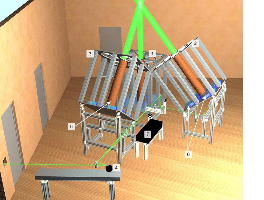
1502                                                  S. M. Khaykin et al.: Doppler lidar at Observatoire de Haute-Provence

Friedman et al., 1997; Gentry et al., 2000; Yan et al., 2017).      idation using OHP lidar; Sect. 6 concludes the study and
The direct-detection technique for wind profiling has been          sketches the outlook.
successfully realized in an airborne Doppler lidar – A2D,
Aeolus Airborne Demonstrator (Reitebuch et al., 2009). The
A2D instrument served as a prototype for the most ambi-
tious endeavor in the context of lidar wind profiling – the first   2     Instrument design and measurement principle
ever satellite-borne Doppler lidar instrument ALADIN (At-
mospheric Laser Doppler INstrument) (ESA, 2008; Stoffelen           A detailed description of the OHP Doppler lidar (LIOvent)
et al., 2005) that has been successfully launched by European       and the methodology for retrieving wind profiles was pro-
Space Agency (ESA) in August 2018 (Kanitz et al., 2019).            vided by Souprayen et al. (1999a). Here, we recap the general
    While the necessity of high-resolution (< 1 km) wind pro-       design of the instrument and its subsystems after its upgrade,
filing of USLM region is well recognized (e.g., Meriwether          the measurement principle and the error budget, as well as
and Gerrard, 2004; Dörnbrack et al., 2017); presently, very         the principal stages of data retrieval.
few instruments with such capacity are operated on a regu-
lar or quasi-regular basis. These are Doppler lidars at Arctic      2.1    Instrument design
Lidar Observatory for Middle Atmospheric Research (ALO-
MAR) in northern Norway (Baumgarten, 2010; Hildebrand               The lidar instrument senses the horizontal wind velocity
et al., 2017), LiWind lidar at high-altitude Maido observa-         by measuring the Doppler shift between the emitted and
tory at Réunion island (Baray et al., 2013; Khaykin et al.,         backscattered light of the laser. The Doppler shift corre-
2018) and LIOvent lidar at Observatoire de Haute-Provence           sponds to the projection of the horizontal wind components
(OHP), where the pioneering lidar measurements of wind up           onto the line of sight of the laser inclined 40◦ off zenith.
to 50 km altitude were conducted by Chanin et al. (1989).           The detection of the Doppler shift is performed by means of
    The OHP wind lidar was originally designed to cover the         a double-edge Fabry–Pérot interferometer (FPI), as detailed
height range of 25–50 km (Garnier and Chanin, 1992), i.e.,          in the following section.
where the contribution of Mie scattering by aerosol parti-             The general design of transmitter–receiver system is
cles can be neglected in most cases. After the eruption of          shown in Fig. 1. The transmitter of the lidar is based on
Pinatubo volcano in 1991 polluting the stratosphere with            a Quanta-Ray Pro290 Q-switched, injection-seeded Nd:YAG
aerosol up to 35 km, the OHP wind lidar was redesigned              laser emitting at 532 nm with a repetition rate of 30 Hz and
to minimize the effect of Mie scattering (Souprayen et al.,         800 mJ per pulse energy. In seeded mode, the linewidth of
1999a,b). The new Rayleigh–Mie Doppler lidar (named LI-             the laser beam is less than 0.003 cm−1 (90 MHz at 532 nm),
Ovent) was deployed at OHP in late 1993 and was oper-               whereas the shot-to-shot frequency stability is better than
ated on a regular basis during 1995–1999. The observations          10 MHz (rms). During the measurement, the laser beam is
were used for retrieval of gravity wave parameters and strato-      commuted successively to each of the three fixed mosaic tele-
spheric wind climatology at OHP (Souprayen et al., 1999a;           scope assemblies, respectively, zenith (1), north (2) and east
Hertzog et al., 2001) as well as for a study of the effect of       (3), using a galvanometric scanner mirror (4). Each telescope
gravity waves on ozone fluctuation in the lower stratosphere        assembly has a field of view of 0.1 mrad and is comprised of
(Gibson-Wilde et al., 1997).                                        a central transmitter shaft with a beam expander (5), ensur-
    After a long period of sporadic operation and limited           ing the beam divergence of 35 µrad (full angle at half maxi-
maintenance, the upgrade of OHP wind lidar was started in           mum) and four collecting parabolic mirrors of 500 mm diam-
2012. At the same time, a similar wind lidar instrument was         eter (6), which translates to the total collective area for each
deployed at Maido observatory at Réunion island and passed          telescope of 0.78 m2 .
a thorough performance evaluation, which will be presented             The backscattered light is collected by means of 200 µm
in a separate paper. The upgrade of both wind lidars included       multimode optical fibers located at the focal point of each
replacement of the laser, optical filtering elements and detec-     mirror (1500 mm focal distance) and linked to an optical
tors. These efforts were largely motivated by the ESA Aeo-          commutation chamber (7), which transfers the collected light
lus satellite mission carrying the ALADIN instrument, which         through a 600 µm fiber from a given telescope to the entrance
exploits the same principle of Doppler shift detection, i.e.,       of the spectral analysis subsystem. The latter (not shown)
the double-edge Fabry–Pérot interferometer (Stoffelen et al.,       comprises the FPI etalon in a thermally stabilized pressure-
2005; Reitebuch, 2012).                                             controlled chamber, a 0.3 nm interference filter for reducing
    This study aims at characterizing the performance and ca-       the sky background and a mode scrambler, which serves for
pacities of OHP LIOvent Doppler lidar after its upgrade. Sec-       homogenizing the incidence angles of light projected onto
tion 2 describes the instrument design; Sect. 3 reports the re-     the FPI. The homogeneity of the flux angular distribution is
sults of LIOvent validation using 12 collocated radiosound-         important because the transmission function of the FPI de-
ings; Sect. 4 provides examples of weekly and hourly obser-         pends on the angular incidence. The scrambler module com-
vation series; Sect. 5 presents an early case of Aeolus val-        prises two lenses, the first collecting the light from the in-

Atmos. Meas. Tech., 13, 1501–1516, 2020                                               www.atmos-meas-tech.net/13/1501/2020/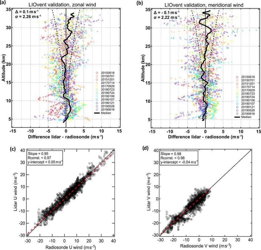
S. M. Khaykin et al.: Doppler lidar at Observatoire de Haute-Provence 1503
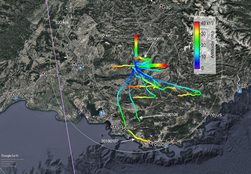
Figure 1. Three-dimensional representation of the transmitter–receiver system of LIOvent lidar comprising three telescope assemblies for
zenith (1), north (2) and east (3) lines of sight with four collecting mirrors (6) and a beam expander (5) each. The emitted laser beam is
commuted between the telescopes using rotating scanner mirror (4). The backscattered light collected by each mirror is transferred via fibers
into the optical commutation chamber (7) for aggregating the fluxes from the four mirrors of each telescope assembly.
put fiber and the second projecting its image onto the output eas with slightly different air gaps, which results in two dis-
fiber. tinct bandpasses on both sides of the Rayleigh–Mie backscat-
The detection of the spectrally processed light is done with tered line, as shown in Fig. 2. The Doppler shift of the
two pairs of cooled super-bialkali Hamamatsu R9880-110 backscattered line (dashed black in Fig. 2) enhances the sig-
photomultipliers (PMTs), receiving, respectively, 95 % and nal transmitted through channel A whilst reducing that of
5 % of the flux (high- and low-gain channels). The high-gain channel B. The interferometer is set in a sealed pressure-
PMTs are electronically gated at 100 µs, i.e., 15 km radial controlled chamber, allowing a spectral tuning of the FPI
distance. The acquisition is done using a four-channel Licel A and B bandpasses relative to the backscattered line through
transient recorder featuring 32 760 gates of 50 ns width (i.e., variation of the air-gap refractive index. Depending on the at-
7.5 m radial resolution). mospheric temperature, the backscattered Rayleigh line ob-
The upgrade of the lidar (with respect to the design de- tains a full width at half maximum (FWHM) between about 2
scribed by Souprayen et al., 1999a) was carried out during and 2.4 pm, whereas the Mie line is assumed to have the same
the 2012–2018 period and included replacement of various spectral width as that of the laser (< 0.08 pm). The spectral
parts. The essential improvements that allowed extending the spacing of the FPI A and B bandpasses of 5.24 pm is deter-
vertical range for wind profiling are due to the following mined by the difference in optical thickness of the respective
upgrades: a higher-power laser (24 vs. 10 W), a new inter- half-disc areas of the interferometer (34.5±0.1 nm), whereas
ference filter (0.3 vs 1 nm) and the new PMTs with faster the FWHM of the FPI bandpasses depends on its finesse and
response and lower dark current. Additionally, a new Licel amounts to 2.03 ± 0.01 pm according to a series of experi-
transient recorder (50 ns vs. 1 µs gate bins) and a new cool- ments by Souprayen et al., (1999a,b).
ing system have been introduced. The Doppler shift response profile R(z, θ ) for a given line
of sight is calculated as
2.2 Doppler shift detection CNA (z, θ ) − NB (z, θ )
R(z, θ ) = , (1)
The detection of Doppler shift is done using a double-edge CNA (z, θ ) + NB (z, θ )
FPI. The FPI etalon (manufactured by StigmaOptique) is as- where NA (z, θ ) and NB (z, θ ) are the number of photons re-
sembled by molecular contact and features two half-disc ar- ceived from altitude z and transmitted through the A and B
www.atmos-meas-tech.net/13/1501/2020/ Atmos. Meas. Tech., 13, 1501–1516, 2020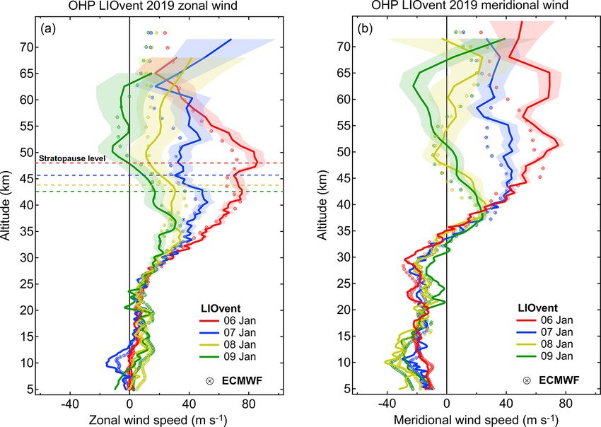
1504                                                   S. M. Khaykin et al.: Doppler lidar at Observatoire de Haute-Provence

                                                                        An absolute measurement of the wind velocity requires
                                                                     a careful determination of the null Doppler shift reference,
                                                                     which is done through 1 min zenith-pointing acquisition
                                                                     within each 5 min cycle. This enables accounting for the pos-
                                                                     sible drift in the emitted laser wavelength, typically of 0.03–
                                                                     0.08 pmh−1 . The horizontal wind components are then ob-
                                                                     tained by subtracting the line-position profile for the ver-
                                                                     tical pointing P (z, 0◦ ) from those of the tilted pointings
                                                                     P (z, 40◦ ):
                                                                                    c     h
                                                                                                     ◦
                                                                                                                    i
                                                                                                                  ◦) ,
                                                                     vh (z) =               P (z, 40   ) − P (z, 0                (2)
                                                                               2λ0 sin40◦

                                                                     where λ0 is the emitted wavelength; and P (z, 0◦ ) is the ref-
                                                                     erence (null Doppler-shift) position given by an average in
                                                                     the altitude range of 15–25 km, a region where the verti-
                                                                     cal wind velocity is negligibly small. Expectedly, the line-
Figure 2. Spectral shapes of the thermally broadened Rayleigh        position profile for the vertical pointing does not vary with
backscatter line with the thin Mie line on top of it (solid black)   altitude; therefore, the resulting wind profiles are insensitive
and the FPI A and B bandpasses (solid red and blue). The Doppler-    to the choice of the vertical range for the null Doppler shift
shifted backscatter line (corresponding to an imaginary wind speed   reference.
of 175 m s−1 ) is shown as dashed black curve. The signals trans-
                                                                        The spectral tuning of the FPI bandpasses with respect to
mitted through the A and B bandpasses for the Doppler-shifted
                                                                     the laser wavelength is verified at the beginning of each mea-
backscattering are illustrated by the dashed red and blue curves.
                                                                     surement session through adjustment of the air pressure in-
                                                                     side the FPI chamber using a stepper motor. The temperature
                                                                     inside the FPI housing module is maintained at 30 ◦ C at all
bandpasses, respectively; and C is the corrective factor ac-         times and we note that over many months of lidar operation,
counting for a possible imbalance between the signals in the         the spectral tuning remains stable, except after an occasional
A and B channels due to a difference in detectors’ sensitiv-         laser maintenance.
ity. The corrective factor corresponds to the ratio between the
A and B channels and is obtained by comparing NA and NB              2.3   Signal processing and statistical uncertainty
signals from a continuous white source. The Doppler shift
(in units of pm) is deduced from the response profile through        The measurement cadence is such that the zenith, north and
the instrumental calibration function, which accounts for the        east lines of sight are alternated in a cycle of 1–2–2 min, re-
temperature broadening of the Rayleigh backscattered line.           spectively. A typical acquisition lasts 5 h during nighttime,
   The procedure of FPI calibration is thoroughly described          that is 2 h integration for each tilted pointing, which ensures
by Souprayen et al. (1999b). Briefly, it makes use of the            signal-to-noise ratio better than 2 all the way up to about
pressure scanning system, which allows for spectral sam-             80 km altitude above sea level (a.s.l.). Figure 3a shows an
pling across the two FPI bandpasses by sequentially shifting         example of raw lidar return profile from the north pointing
their spectral position with respect to the spectrally stable        obtained by stitching the low- and high-gain signals. The ver-
laser line. With the constant and known spectral spacing be-         tical range of the useful signal spans between about 5 and
tween FPI bandpasses, one can relate the scanner motor steps         80 km. The lower boundary is due to strong returns from the
to the unit of pm. This relation is then used to retrieve the        lower troposphere saturating the detectors in addition to an
FWHM of each bandpass, which, together with the FPI spec-            incomplete geometrical overlap below 2 km.
tral spacing and temperature-dependent spectral width of the            The photons received from the transient recorder are ag-
backscattered line, yields the instrumental calibration func-        gregated over 1 min intervals and downsampled to 1 µs bins
tion. The calibration function is linear in the central zone (be-    (150 m radial resolution). The offline signal pre-processing
tween −0.2 and 0.2 pm) and obtains the slope of 0.755 pm−1           includes subtraction of background due to sky light and PMT
at 210 K. The uncertainty in the FPI characteristics induces         thermal noise as well as dead-time correction, after which
an uncertainty of ±0.3 % on the horizontal wind velocity,            the response profiles are calculated for each line of sight ac-
whereas the effect of temperature uncertainties does not ex-         cording to Eq. (1). Then, the Doppler shift (line-position pro-
ceed 0.07 % per K (Souprayen et al., 1999a). Since the FPI           file) is computed using the instrument calibration function
is placed in a sealed chamber, its spectral characteristics re-      with account for atmospheric temperature profile, provided
main constant with time, and the calibration through pressure        by operational analysis by the European Centre for Medium-
scanning is needed only if upgrading the laser unit or the op-       Range Weather Forecasts (ECMWF). Finally, the zonal and
tical processing box.                                                meridional wind components are obtained by comparing the

Atmos. Meas. Tech., 13, 1501–1516, 2020                                                www.atmos-meas-tech.net/13/1501/2020/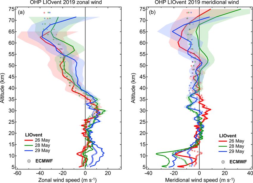
S. M. Khaykin et al.: Doppler lidar at Observatoire de Haute-Provence 1505
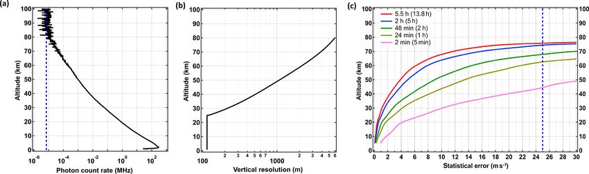
Figure 3. (a) Nightly average raw signal vertical profile obtained in a 7 h lidar acquisition on 28 January 2019. The dashed blue curve
indicates the background noise level. (b) Altitude-variable vertical resolution used in the retrieval. (c) Statistical error profiles computed for
different acquisition times of a tilted (north) pointing. The values in brackets correspond to the total duration of lidar acquisition, including
zenith, north and east pointings in a cycle of 1–2–2 min. The dashed blue line marks the cut-off error threshold.
tilted east and north pointings to the corresponding zenith 3 Comparison with collocated radiosoundings
pointing using Eq. (2).
Statistical error due to Poisson noise (shot error) in-
Over the 4-year period, spanning June 2015 to June 2019, the
creases with altitude proportionally to the exponential decay
√ validation of the LIOvent wind lidar was conducted using 12
of molecular backscatter. As the error scales with 1/ 1z
radiosonde (RS) ascents performed at OHP during the time
(where 1z is the vertical resolution), we use a height-
of lidar acquisition. We used Meteomodem M10 radiosondes
dependent 1z, which is set to 115 m (150 m radial) below
equipped with Global Navigation Satellite Systems (GNSS)
25 km and then increased quasi-exponentially with altitude,
receiver, launched under TOTEX 1200 g weather balloons.
from 500 m at 40 km to 4000 m at 70 km (Fig. 3b). For
The balloons reached on average 29.9 km altitude, whereas
a given vertical resolution, we compute the statistical error
the horizontal drift during ascent did not exceed 90 km from
(m s−1 ) of an individual response profile:
the launch point.
Figure 4 displays the altitude-coded trajectories of the 12
p radiosonde ascents as well as the ground projections of LI-
NA (NB − F cB )2 + NB (NA − F cA )2 Ovent tilted pointings. The horizontal displacement of the
σR = 2C , (3)
[C(NA − F cA ) + (NB − F cB )]2 radiosondes with respect to the lidar sampling location at ev-
ery altitude level was calculated separately for the east and
north pointings and amounted, respectively, to 27 ± 19.5 km
where F cA and F cB are the background signals in chan- and 39 ± 25 km (1σ ), the largest being 117 km for the north
nels A and B, and C is the corrective factor introduced in pointing. Generally, the displacement increased with altitude
the previous section. as the balloons were drifting away from the lidar sampling
Figure 3c shows the altitude profiles of statistical error for locations, as Fig. 4 suggests.
different integration times. For a typical lidar acquisition last- For setting up the intercomparison, lidar measurements
ing 5 h (i.e., 2 h of a given tilted pointing acquisition, blue were averaged over the time period of radiosonde ascent
curve), the statistical error is less than 2 m s−1 below 33 km (110 min from the ground to 33 km altitude at 5 m s−1 as-
and does not exceed 6 m s−1 throughout the stratosphere. In cent rate), whereas the radiosonde measurements, reported
the mesosphere, the error increases from 6 m s−1 at 55 km at 1 Hz frequency, were downsampled to match the vertical
to 16 m s−1 at 70 km. A longer acquisition (13.8 h, red curve) resolution of lidar profiles (115–320 m depending on the al-
reduces the error yet does not extend the vertical coverage: at titude). The results of intercomparison are reported in Ta-
75 km altitude, the statistical errors for 5 and 13.8 h acquisi- ble 1 as absolute difference between RS and LIOvent wind
tion are nearly the same. We use the statistical error value of profiles, standard deviation of the differences and correlation
25 m s−1 as a threshold for cut-off altitude of retrieved wind for each particular sounding. The intercomparison exercise
profiles. Given such a threshold, the top of vertical range for is done separately for the zonal and meridional wind compo-
a standard (5 h) lidar acquisition is ∼ 75 km, whereas a 5 min nents as well as for the total wind speed and wind direction.
acquisition (pink curve), corresponding to a single north– The mean differences obtained from the individual com-
east–zenith measurement cycle, enables coverage up to about parison cases vary between −1.3 and 0.9 m s−1 for zonal
44 km. wind and between −2 and 0.9 m s−1 for meridional wind.
www.atmos-meas-tech.net/13/1501/2020/ Atmos. Meas. Tech., 13, 1501–1516, 2020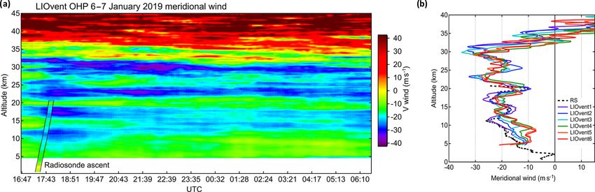
1506                                                    S. M. Khaykin et al.: Doppler lidar at Observatoire de Haute-Provence

Figure 4. OHP wind lidar sampling location along north and east lines of sight (thick lines) and trajectories of 12 radiosondes launched
from OHP for wind lidar validation (thinner curves) color coded by the altitude a.s.l. Grey circles indicate the distance from OHP. Particular
radiosonde flights are tagged by white arrows with an indication of the flight date. The magenta line shows the ground track of Aeolus lidar
(see Sect. 5). © Google Earth.

For the total wind and direction, the differences vary between              The mean standard deviation of the differences for the 12
−1.1 and 0.7 m s−1 and between −4.9 and 9.6◦ , respectively.             collocated soundings amounts to 2.26 m s−1 for the zonal and
The averages of all intercomparison cases amount to +0.1                 2.22 m s−1 for the meridional wind profiles. These values are
and −0.1 m s−1 , respectively, for the zonal and meridional              consistent with the estimated shot error for a 2 h lidar ac-
components, 0.0 m s−1 for the total wind and 0.3◦ for the                quisition (i.e., duration of a radiosounding), which increases
wind direction.                                                          from 0.2 to 3.4 m s−1 in the altitude range of lidar–radiosonde
   Figure 5a and b show altitude profiles of the absolute dif-           intercomparison, as can be inferred from Fig. 5a, b. For eval-
ference between LIOvent and RS for each sounding as well                 uating the effect of the horizontal offset between the lidar
as the median profile. The point-by-point differences rarely             and RS measurements, we computed the offset-weighted av-
exceed 5 m s−1 , whereas the median values never exceed                  erages of the intercomparison statistics and compared them
2 m s−1 . While the median difference profiles do not indi-              with the ordinary averages. The weight for each individual
cate any altitude-dependent bias, the scatter of differences             value is defined as w = 1 − D̄/Dmax , where D̄ is the mean
appears to increase with altitude. This is due, on one hand, to          distance between the lidar and RS sampling locations, and
larger horizontal offset between measurements at higher alti-            Dmax is the maximum distance amounting to 69 km (Ta-
tudes and, on the other hand, due to an increase of statistical          ble 1). We note that the horizontal-offset weighting of the
error with altitude shown as dashed curves in Fig. 5a and b.             differences neither affects the mean difference nor the mean
   The bottom panels of Fig. 5 display the scatter plots of              correlation but reduces the standard deviation for the wind
the wind velocities measured by the lidar and the radioson-              components and total wind by about 0.2 m s−1 . This suggests
des with associated regressions and correlation coefficients.            that horizontal variability of the wind field on a scale of few
For both wind components, the slope of the regression line is            tens of kilometers is small yet non-negligible.
close to 1, which affirms the credibility of the FPI calibration            Figure 6 presents examples of summer and winter zonal
function relating the Doppler shift response to wind veloc-              wind intercomparison cases, both showing directional wind
ity. The Pearson correlation coefficient r deduced from the              shear in the lower stratosphere but of opposite sign. Re-
ensemble of collocated measurements amounted to 0.97 and                 markably, the small-scale fluctuations, presumably caused by
0.96, respectively, for zonal and meridional wind velocities,            gravity waves propagation and/or breaking, are reproduced
0.97 for the total wind and 0.89 for the wind direction.                 by the lidar just as accurately as they are measured by the
                                                                         balloon sonde carried by those winds.

Atmos. Meas. Tech., 13, 1501–1516, 2020                                                      www.atmos-meas-tech.net/13/1501/2020/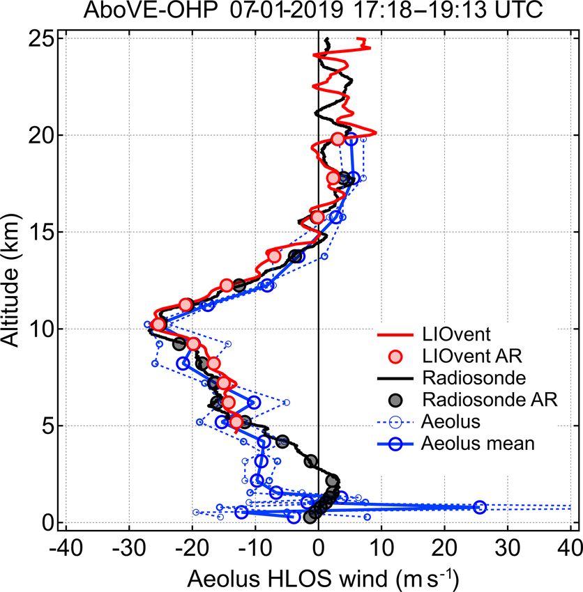
S. M. Khaykin et al.: Doppler lidar at Observatoire de Haute-Provence                                                                 1507

Table 1. Summary of intercomparison between LIOvent lidar and time-collocated radiosoundings launched at OHP. The results are shown
separately for zonal (U ) and meridional (V ) wind measurements as well as for the total wind speed (Vh ) and wind direction (ϕ). Provided
for each case of intercomparison (from left to right) are measurement date, mean absolute difference, standard deviation of the differences,
Pearson’s correlation coefficient (r), mean horizontal distance between the lidar and radiosonde sampling locations and top altitude of
radiosounding. The average values are provided in the bottom row.

   Date                   Mean difference,                     SD                        Correlation            Distance,    Top of RS,
                         m s−1 or degrees (ϕ)          m s−1 or degrees (ϕ)              coefficient r             km               km
                       U        V      Vh        ϕ     U     V     Vh       ϕ      U       V       Vh      8    U      V           Ztop
   18 Jun 2015      −1.3     0.1     −0.9     2.9     2.9   2.3    2.6   16.8    0.95    0.96    0.97    0.93   31     47          32.5
   1 Jul 2015        0.9    −0.8     −0.1    −4.1     2.1   1.2    2.4   13.5    0.92    0.89    0.96    0.95   16     21          28.0
   1 Dec 2015       −0.4     0.6     −0.2    −1.4     1.8   2.0    1.9   18.9    0.96    0.96    0.98    0.92   15     27          33.0
   14 Jul 2017       0.1    −0.3      0.5     1.9     2.6   3.1    2.5   20.3    0.98    0.79    0.99    0.96   46     69          33.0
   29 Sep 2017      −0.0    0.65      0.3    −4.6     2.7   2.7    2.5   27.8    0.93    0.85    0.96    0.75   18     38          33.0
   23 Jul 2018      0.29     0.1     −0.3     0.9     3.2   2.9    2.5   19.4    0.97    0.88    0.98    0.94   21     38          37.3
   24 Jul 2018       0.2     0.0      0.5    −2.0     1.6   1.3    1.5   14.6    0.99    0.89    0.99    0.97    8     22          20.1
   6 Jan 2019       −0.1     0.9     −1.1     0.5     2.5   2.1    3.4   10.7    0.90    0.99    0.98    0.91   37     45          20.9
   7 Jan 2019        0.4    −0.7      0.7    −0.0     2.9   3.8    3.0    8.4    0.98    0.98    0.99    0.98   57     67          33.5
   21 Jan 2019       0.1     0.0      0.2    −1.7     0.9   1.5    1.2    6.7    0.99    0.98    0.99    0.99   13     20          18.0
   28 May 2019      −0.2    −2.0      0.4     9.6     2.7   3.6    2.6   24.8    0.94    0.89    0.97    0.71   27     49          32.5
   16 Jun 2019       0.6    −0.5      0.3     1.3     2.5   2.5    2.0   20.9    0.94    0.72    0.96    0.73   12     15            37
   Average            0.1   −0.1       0.0      0.3   2.3   2.2    2.3   16.9    0.97    0.96    0.97    0.89   27     35          29.9

   At higher altitudes, the fine-scale fluctuations resolved by          2.4 pm), the intensity of the former may be substantially
the lidar appear at times out of phase with those seen by                higher and thereby alter the spectral shape of the return sig-
the radiosonde. This is more prominent in the summer case                nal. In this case, a disproportionally larger flux would be
(Fig. 6a) despite the closer collocation of the measurements.            transmitted through one of the FPI bandpasses, affecting its
In this case, the RS ascent closely follows the lidar’s line of          calibration function and introducing a bias into the wind re-
sight up until 19 km (see Fig. 4), while the LIOvent zonal               trieval within the particle layer. The sensitivity to Mie scat-
profile precisely tracks the one of RS up to about the same              tering can be reduced by increasing the FPI spectral spac-
level. At 19 km, the zonal wind reverses, the balloon makes              ing; however, this also reduces the sensitivity to the Doppler
a U turn and progressively drifts westward and away from the             shift. The optimal spectral configuration of the FPI has been
lidar. Above 30 km, the RS and LIOvent profiles start to get             established on the basis of a theoretical model by Souprayen
out of phase whilst both showing an increasing easterly wind             et al. (1999b). They found that for observable stratospheric
between 30 and 35 km. The lidar profile, extending above the             wind velocities, the residual Mie-induced error is less than
top of radiosounding, reveals a typical signature of a gravity           1 m s−1 for the scattering ratio of R = 10, which is charac-
wave, supposedly propagating in the zonal direction (consid-             teristic of a cirrus cloud readily visible to an unaided eye.
ering a relatively unperturbed meridional wind profile in this              In this study, we have experimentally revisited the aspect
layer; not shown).                                                       of FPI sensitivity to particulate scattering. The eruption of the
   While the statistical error of the lidar measurement be-              Raikoke stratovolcano (22 June 2019, Kuril Islands; 48◦ N,
comes comparable to the observed variations at these lev-                153◦ E) has polluted the lower stratosphere with a large
els, the dephasing of LIOvent and RS profiles in Fig. 6a is              amount of sulfuric aerosol (NASA Earth Observatory, 2019).
likely due to spatially offset sampling of the gravity wave              The aerosol plumes were observed by OHP lidars every night
front. Interestingly, the dephasing above 30 km is less obvi-            since 10 July 2019 (and at the time of writing) between 12
ous in the winter case (Fig. 6b) despite a considerably larger           and 20 km altitude, which provided an opportunity for testing
spatial offset, compared to the summer case (88 vs. 36 km).              the sensitivity of wind lidar to Mie scattering in the strato-
This may be explained in consideration of the much stronger              sphere.
zonal wind in the winter case (38 vs. −2 m s−1 ), damping the               Figure 7 displays lidar measurements of aerosol scatter-
amplitude of the wave-induced perturbations.                             ing ratio (SR) and zonal wind velocity on 20 July. The SR
                                                                         profiles were obtained from an aerosol channel (532 nm)
Sensitivity to Mie scattering                                            of the LTA (lidar temperature aerosol) instrument (Keckhut
                                                                         et al., 1993) and from the zenith acquisition of LIOvent li-
Although the Mie-backscattered line is narrow (0.08 pm)                  dar using the aerosol retrieval method described by Khaykin
compared to the thermally broadened Rayleigh line (2–

www.atmos-meas-tech.net/13/1501/2020/                                                      Atmos. Meas. Tech., 13, 1501–1516, 2020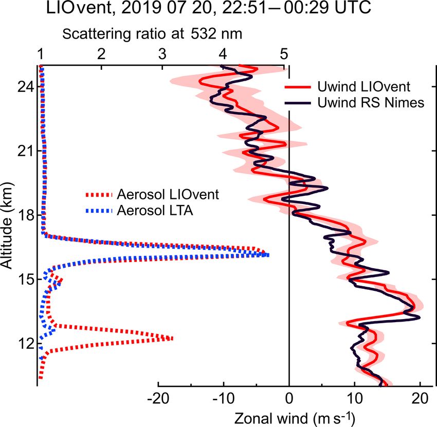
1508                                                      S. M. Khaykin et al.: Doppler lidar at Observatoire de Haute-Provence

Figure 5. Summary of LIOvent lidar validation using radiosonde ascents from OHP. Absolute difference between LIOvent and radiosonde
zonal (a) and meridional (b) wind velocity for each sounding (colored circles representing various dates; dates provided in the legend) and
median profile (black curve). The dashed line indicates the statistical uncertainty estimated for a 2 h lidar acquisition. The mean difference
(1) and the mean standard deviation of the difference (σ ) are indicated in the top-left corner of panels (a, b). Scatter plots of the zonal (c)
and meridional (d) wind velocities measured by the lidar and the radiosondes. The 1 : 1 line is solid black; the linear regression line is dashed
red.

Figure 6. Selected cases of the lidar–radiosonde intercomparison of the zonal wind profiles in June (a) and January (b) 2019. The lidar
measurement dates and times are given above the panels; the time of radiosonde launch on the same date is provided in the legend.

Atmos. Meas. Tech., 13, 1501–1516, 2020                                                        www.atmos-meas-tech.net/13/1501/2020/
S. M. Khaykin et al.: Doppler lidar at Observatoire de Haute-Provence                                                            1509

                                                                        4     Observations

                                                                        During the 2015–2019 period, the LIOvent instrument was
                                                                        operated on 52 nights, mostly during early summer and
                                                                        winter seasons. This section reports examples of successive
                                                                        nightly mean profiles reflecting the wind variability in the
                                                                        middle atmosphere during opposite seasons as well as a par-
                                                                        ticular case of temporally resolved wind profiling.

                                                                        4.1    January 2019 series

                                                                        An interesting dynamical event in the USLM was observed
                                                                        in January 2019 during an intensive measurement campaign
                                                                        dedicated to Aeolus validation (AboVE-OHP, Aeolus Valida-
                                                                        tion Experiment at OHP). A strong perturbation of the Arctic
                                                                        circumpolar vortex occurred as a result of a major sudden
                                                                        stratospheric warming event during the first week of Jan-
                                                                        uary 2019. According to potential vorticity maps (not shown)
Figure 7. Zonal wind profiles (bottom axis) measured by the             based on ECMWF Integrated Forecast System (IFS), the vor-
LIOvent wind lidar (solid red) and by MeteoFrance routine ra-           tex started to split around 1 January and evolved into two sep-
diosounding launched from Nimes airport (100 km away from               arate vortices above Europe and Canada by 4 January. The
OHP; see Fig. 4) at 00:00 UTC on 21 July 2019 (solid black). The        European counterpart was displaced southward and its edge
date and time of LIOvent measurement is shown at the panel top.
                                                                        – at 850 K potential temperature level (∼ 50 km) – reached
The aerosol scattering ratio profiles obtained using LIOvent zenith
pointing (dashed red) and LTA lidar (dashed blue), showing the vol-
                                                                        OHP around 6 January, that is when the AboVE-OHP mea-
canic aerosol layer at 16.2 km, are plotted in the top axis. See text   surement campaign was started.
for details.                                                               Figure 8 shows ensembles of the zonal and meridional
                                                                        wind profiles obtained during the 6–9 January period. The
                                                                        plots include indications of the stratopause level, which was
et al. (2017, and references therein). The LIOvent operation            progressively descending from 47 to 43 km during that pe-
was started after the end of LTA operation since the lidars             riod, as inferred from simultaneous temperature profiling us-
share the same laser and cannot be operated simultaneously.             ing LiO3S (Lidar O3 stratosphérique) differential absorption
Both lidars consistently show an aerosol layer at 16.2 km al-           lidar (Godin-Beekmann et al., 2003; Wing et al., 2018). The
titude with SR reaching 4.7 and an estimated optical depth              6 January wind profiles (red curves) reflect the perturbed
of 0.03, which is comparable to a thin cirrus cloud (Hoareau            conditions when the vortex edge was located above OHP and
et al., 2013). In addition, the LIOvent measurement reveals             both zonal and meridional components were maximizing at
a cirrus cloud at 12.2 km, which occurred only towards the              80 m s−1 around the stratopause. As the edge of vortex was
end of LTA acquisition and thereby left a weaker imprint in             moving back north of OHP during the following days, the
the average SR profile of LTA.                                          measurements show weakening winds throughout the USLM
   The LIOvent wind measurement in the presence of ice                  and reversal of both wind components in the lower meso-
crystals and volcanic aerosol is compared in Fig. 7 to a time-          sphere by 9 January. The rapidly weakening winds form an
collocated radiosoundings conducted from Nimes airport,                 envelope of profiles with a bottom at ∼ 27 km for the zonal
situated ∼ 100 km west from OHP (see Fig. 4). While the                 wind and ∼ 38 km for the meridional component. Below this
vertical structures in the LIOvent and RS wind profiles are             envelope, neither of the wind components show significant
at times out of phase (which may be explained by spatial                change over the 4 d period.
variability), the lidar profile does not show any indications              The observed evolution of wind profiles is reproduced by
of Mie-induced bias, neither due to a thin cirrus cloud nor             the ECMWF T1279/L137 operational analysis represented
due to a volcanic aerosol layer. Such a bias would appear as            by cross circles in Fig. 8. The wind change envelope and
a sharp feature in the wind profile coinciding with the SR en-          the vertical structure of the wind profiles are both well re-
hancement, which is obviously not the case here. This result            solved by the model. The ECMWF profiles reproduce the ob-
confirms that the spectral configuration of the FPI allows ac-          served vertical fluctuations on a scale of a few kilometers up
curate wind measurements in the presence of particles in the            to the stratopause, which is remarkable since the regular ra-
middle atmosphere.                                                      diosoundings assimilated into the model hardly reach 30 km
                                                                        altitude. We note that the consistency between ECMWF and
                                                                        LIOvent is better for the zonal wind, whereas the vertical
                                                                        structures in meridional wind are somewhat less consistent

www.atmos-meas-tech.net/13/1501/2020/                                                    Atmos. Meas. Tech., 13, 1501–1516, 2020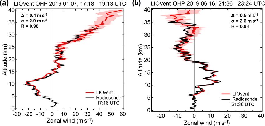
1510                                                  S. M. Khaykin et al.: Doppler lidar at Observatoire de Haute-Provence

Figure 8. Ensembles of nightly mean vertical profiles of zonal (a) and meridional (b) wind profiles obtained by LIOvent in January 2019
(solid curves) with statistical uncertainty shown as shading and the corresponding ECMWF IFS profiles (cross circles). Horizontal dashed
lines in the left panel indicate the stratopause altitude obtained from simultaneous temperature lidar measurements.

Figure 9. Same as Fig. 8 but for May 2019.

Atmos. Meas. Tech., 13, 1501–1516, 2020                                                  www.atmos-meas-tech.net/13/1501/2020/
S. M. Khaykin et al.: Doppler lidar at Observatoire de Haute-Provence                                                              1511

Figure 10. (a) Temporal variation of the meridional wind profile over the course of a continuous whole-night LIOvent acquisition started
on 6 January 2019. Superimposed onto the lidar time–altitude section is the corresponding radiosonde ascent from OHP, plotted using the
same color map as the lidar wind curtain. (b) Successive 135 min averages of meridional wind measured by the lidar (solid curves) and the
radiosonde profile (dashed black).

with the observations in the USLM. Analogous results, in-              the collecting mirrors of the north-pointing telescope assem-
ferred from intercomparison between ALOMAR wind lidar                  bly.
and ECMWF forecast winds, were reported by Rüfenacht
et al. (2018). The damping and dephasing of the vertical               4.3   Time-resolved wind profiling
structures by ECMWF becomes more prominent above about
50 km, which might be due to both the temporal averaging               An important advantage of the Doppler lidar technique is
over 5–13 h by the lidar and the coarse model resolution in            the capacity to provide temporally resolved vertical profiling
the mesosphere. A detailed comparison between wind lidar               of the atmosphere, which enables characterization of high-
observations, ECMWF IFS and reanalysis data will be the                frequency fluctuations in the wind profile, inaccessible with
subject of a separate study.                                           snapshot-like radiosonde measurements. Figure 10a provides
                                                                       an example of meridional wind profile variation over the
4.2   May 2019 series                                                  course of a continuous whole-night lidar acquisition lasting
                                                                       nearly 14 h. Superimposed onto the lidar time–altitude sec-
Figure 9 shows a sequence of wind profiles acquired during             tion is a radiosonde ascent, plotted using the same color map
late May 2019. While the winds appear highly variable in the           as the lidar wind curtain.
upper troposphere due to the dynamics of the jet stream, the              The LIOvent and RS profiles are remarkably consistent,
middle stratosphere remains relatively calm and stable over            as can be seen from the color map (correlation coefficient
the considered 4 d period. The zonal wind reverses at around           amounts to 0.99 in this case). With that, the lidar wind cur-
36 km and the easterlies pick up until ∼ 65 km, that is when           tain shows important variation of the wind velocity over the
the wind shear reverses. The meridional wind is very weak              course of 14 h acquisition. The peak-to-peak variation at any
throughout the stratosphere except for a small envelope at             level below 30 km altitude is between 10 and 20 m s−1 , in-
30 km, which accompanies the zonal wind perturbations in               creasing to ∼ 30 m s−1 towards 40 km. The wind change rate
this layer. The ECMWF IFS accurately resolves this enve-               in any 3 km thick layer is reaching 10 m s−1 per hour, which
lope; however, the observed vertical structures above, in the          points to the predominance of temporal variability of the
USLM, are not reproduced by the model. In particular, the              wind field over its spatial variability. Indeed, the maximum
reversal of wind shear at around 65 km in both wind com-               deviation of the lidar profile from the RS one in this case did
ponents is missed by the model, whereas the lidar profiles             not exceed 4 m s−1 at any given level, all the while that the
consistently report this feature, significant at the permitted         RS measurements were taken as far as 71 km away from the
statistical error of 25 m s−1 .                                        lidar sampling location (see Fig. 4).
   The imposed error threshold of 25 m s−1 determines the                 In the upper-middle stratosphere (i.e., around 35 km),
cut-off altitude of the wind profiles reported in Figs. 8 and          where the meridional wind reverses, one can discern wind
9. The top altitude varies between 65 and 75 km depending              patterns slowly propagating downward. This pattern is a typ-
on the presence of cirrus clouds inhibiting the return signal          ical signature of upward-propagating gravity waves with
from above. We note that the meridional profiles normally              a non-zero ground-based phase speed. A somewhat differ-
reach higher altitudes, which is due to a better condition of          ent pattern is observed in the lower-middle stratosphere (15–

www.atmos-meas-tech.net/13/1501/2020/                                                    Atmos. Meas. Tech., 13, 1501–1516, 2020
1512 S. M. Khaykin et al.: Doppler lidar at Observatoire de Haute-Provence
vertical wavelength λz can be deduced from the horizontal
wind speed vh and the buoyancy frequency N :
vh
λz = 2π . (4)
N
Given the observed vh ∼ 20 m s−1 and N ∼ 0.02 s−1 , we ob-
tain the vertical wavelength of ∼ 6.5 km, which corresponds
well to what can be deduced directly from the wind profiles
in Fig. 10.
5 First results of Aeolus validation
Aeolus is the ESA’s satellite mission designed to measure
wind and aerosol profiles in the troposphere and lower strato-
sphere on a global scale (Stoffelen et al., 2005; ESA, 2008).
Launched on 22 August 2018, the Aeolus satellite carries
ALADIN, which features a telescope of 1.5 m diameter and
a laser emitting at 355 nm with a repetition rate of 50 Hz and
Figure 11. Example of the validation of preliminary L2B HLOS
∼ 65 mJ per pulse energy (Reitebuch et al., 2019). The AL-
wind of the ESA Aeolus ALADIN lidar using the LIOvent lidar
and a radiosounding within AboVE-OHP campaign. The LIOvent
ADIN instrument has two detection channels for measuring
and RS wind components are converted to Aeolus HLOS wind and Doppler shift using the molecular (Rayleigh) and particu-
reported at their native vertical resolution (solid red and black) as late (Mie) backscattering. The Rayleigh channel makes use
well as after downsampling to Aeolus vertical resolution (circles, of a double-edge Fabry–Pérot interferometer, which is the
marked AR in the legend). The Aeolus overpass near OHP took measurement principle exploited by the OHP wind lidar.
place on 7 January 2019 at 17:50 UTC (ascending orbit). The mean The ALADIN telescope is pointed 35◦ away from the or-
distance between the LIOvent and ALADIN sampling locations is bital plane in order to sense the backscattered light perpen-
106 km. The lidar acquisition time (corresponding to the radiosonde dicular to the trajectory of the satellite. This enables measur-
ascent time) is provided at the top of the panel. See text for further ing the so-called horizontal line-of-sight (HLOS) wind ve-
details. locity, which is close to the zonal wind component except at
high latitudes. The Aeolus satellite has a Sun-synchronous
dusk–dawn orbit with a 7 d repeat cycle, passing near the
30 km), where the vertical structures appear to remain con- OHP station (within 100 km) twice per week along the suc-
stant with altitude. Figure 10b provides a deeper insight into cessive ascending and descending orbits, at around 17:50 and
the variable structure of this layer by showing a sequence 05:50 UTC, respectively.
of six wind profiles, obtained by integrating over successive As Aeolus and the OHP wind lidar exploit the same mea-
135 min temporal intervals as well as the corresponding RS surement technique, the LIOvent instrument is an important
profile. One can see three layers of stronger southward wind contributor to Aeolus cal/val activity. Starting from January
at around 17, 23 and 30 km altitude interleaved by two layers 2019, and by the time of writing, LIOvent has been oper-
of weaker wind at around 20 and 26 km. ated on 27 nights, providing eight measurements collocated
The persistence of the observed structures in both tempo- with Aeolus overpasses. Some of the Aeolus-collocated LI-
ral and vertical dimensions suggests the occurrence of sta- Ovent acquisitions were accompanied by simultaneous ra-
tionary gravity waves, most likely generated by the flow over diosonde ascents. While a comprehensive validation exercise
the Alps. Indeed, the circulation in the lower troposphere at will be the subject of a separate study, here we provide an
that time (not shown) was such that the OHP site was down- example of comparison between collocated Aeolus level 2B
wind of the Alps. The stationary gravity waves, generated by B02 “Rayleigh-clear” and LIOvent wind profiles. One should
the flow over the mountain range, could propagate freely into bear in mind that Aeolus wind data processing is still being
the stratosphere because of the absence of directional wind improved by optimizing the in-obit instrument calibration;
shear all the way up to 35 km. The amplitude of these wave- therefore, the presented validation case is to be considered as
induced perturbations appears to increase with altitude from preliminary.
∼ 5 to ∼ 10 m s−1 , which is expected from the linear theory Figure 11 displays a collocation case from 7 January
of atmospheric waves. 2019 when the satellite was sampling the atmosphere around
The orographic nature of the gravity wave, identified using 100 km west of OHP along the ascending orbit. The plot in-
time-resolved lidar measurements, can be verified in consid- cludes two successive Aeolus wind profiles (dashed blue) ob-
eration of the vertical wavelength. For a stationary wave, the tained by 12 s integration (i.e., 90 km along-track distance) as
Atmos. Meas. Tech., 13, 1501–1516, 2020 www.atmos-meas-tech.net/13/1501/2020/S. M. Khaykin et al.: Doppler lidar at Observatoire de Haute-Provence 1513
well as their mean (solid blue). The LIOvent and RS wind ments amounted to 0.97 for the total wind speed and to 0.89
components are converted to Aeolus HLOS wind and re- for the wind direction.
ported at their native vertical resolution (solid red and black) We have shown that wind profiling with the LIOvent lidar
as well as after downsampling to Aeolus vertical resolution has little or no sensitivity to the presence of particles (thin
(circles). cirrus clouds or stratospheric aerosols) and we have demon-
The profiles are found to be in good agreement, con- strated the capacity of the wind lidar to measure vertical pro-
sistently reproducing the peak in the eastward wind of files of aerosol backscattering. In addition, using the three
−25 m s−1 at 10 km, which corresponds to an anticyclonic different lines of sight, one can obtain information on the
feature of the jet stream (not shown). In the middle tropo- fine-scale horizontal variability of stratospheric aerosol.
sphere, successive Aeolus profiles appear somewhat scat- The examples of successive nightly mean wind profiles
tered around their mean, with the latter being in better agree- given in Sect. 4.1 and 4.2 provide interesting examples of the
ment with the ground-based measurements. Below 5 km, the wind variability in the upper stratosphere and lower meso-
Aeolus profile deviates from the RS, which may be caused sphere, the atmospheric layer of exceptionally poor obser-
by a stronger spatial variability of the wind field in the lower vational coverage. The observed vertical structures and the
troposphere (note that the minimum horizontal distance be- rapidly changing wind shear reflect the complex dynam-
tween the RS and Aeolus measurements is 91 km). In the ics of the USLM layer and its two-way interactions with
lower stratosphere, that is, above about 11 km, Aeolus fol- the upward-propagating gravity waves, whose manifestation
lows well the downsampled measurements by OHP lidar and may be not well reproduced by atmospheric models. We note
radiosonde. The average difference between the mean Aeolus though that ECMWF operational model tends to reproduce,
and downsampled LIOvent HLOS wind profiles in the over- in most cases, the observed vertical structures at least up to
lapping range of 5–20 km amounts in this case to +1.5 m s−1 50 km altitude.
with a standard deviation of 3.2 m s−1 and a correlation coef- The example of time-resolved wind profiling presented in
ficient of 0.96. Similar values were obtained from other col- Sect. 4.3 highlights the capacity of the LIOvent instrument
locations during AboVE-OHP campaign in January 2019. to detect high-frequency fluctuations in the wind profile, in-
dicative of various types of gravity waves. This rare capac-
ity enables a comprehensive characterization of the high-
6 Summary and outlook frequency part of the wave spectrum, inaccessible with any
other measurement technique. At OHP, the wind lidar acqui-
The OHP wind lidar presented here was a unique instrument sitions are typically accompanied by temperature profiling
at the time of its creation and remains one of the very few in- using Rayleigh lidar, which altogether provides a complete
struments capable of wind profiling in the middle atmosphere suite of thermodynamical parameters in the middle atmo-
with vertical resolution up to 115 m and temporal resolution sphere on a regular basis and for a long term.
up to 5 min. In this paper, we have described the design of the Using the time-resolved wind profiling and simultaneous
instrument after its upgrade and evaluated its capacities us- radiosoundings, we have found that the temporal variability
ing a dozen time-collocated radiosoundings launched from of wind profile in the free atmosphere at a scale of 1 h may
OHP. We have shown that the lidar is capable of measur- be at least twice as large as the spatial variability on a scale
ing horizontal wind velocity between 5 and 75 km altitude of 50–100 km, as deduced from the lidar–radiosonde inter-
with a random error of less than 6 m s−1 up to the top of comparison. This finding is to be considered for Aeolus wind
the stratosphere. We note that the vertical range can poten- validation activities in a sense that a precise temporal collo-
tially be extended to 3–80 km through replacement of the cation may be more important than the spatial collocation of
beam-commuting and beam-splitting mirrors, for which the the wind measurements.
resources are available. We have presented the first preliminary case of Aeolus val-
A noticeable result of the lidar–radiosonde intercompar- idation using the LIOvent lidar. We note that while the Aeo-
ison is a remarkably small average bias of ±0.1 m s−1 for lus data processing and calibration may be subject to further
both wind components and 0.3◦ for the wind direction. This improvement, the first results of intercomparison between the
finding affirms the reliability of the on-the-run calibration ground-based and space-borne Doppler lidars are encourag-
(through periodical zenith pointing) as well as the stabil- ing. The validation of Aeolus is to be continued at OHP on
ity of the FPI calibration function. Also remarkable is that a regular basis for monitoring of the long-term stability of the
the small-scale wind fluctuations are reproduced by the lidar satellite lidar, whereas a dedicated Aeolus validation study
just as accurately as they are measured by the balloon son- will be provided in a separate article.
des carried by those winds. The average standard deviation Further studies exploiting LIOvent observations will ad-
of the differences for the total horizontal wind was found to dress the characteristics of gravity waves retrieved from si-
be only ∼ 2.3 m s−1 , which is consistent with the error esti- multaneous wind and temperature profiling at OHP, as well
mates for the considered altitude range. The correlation co- as intercomparison with operational analysis and new reanal-
efficient obtained from the ensemble of collocated measure- ysis data sets such as ECMWF ERA5. The lidar wind profil-
www.atmos-meas-tech.net/13/1501/2020/ Atmos. Meas. Tech., 13, 1501–1516, 20201514 S. M. Khaykin et al.: Doppler lidar at Observatoire de Haute-Provence
ing is also to be used in conjunction with infrasound mea- References
surements carried out at OHP (Le Pichon et al., 2015) for
studies of middle atmosphere dynamics.
Abreu, V. J., Barnes, J. E., and Hays, P. B.: Observations of winds
with an incoherent lidar detector, Appl. Optics, 31, 4509–4514,
1992.
Data availability. The wind lidar data are available through the
Baray, J.-L., Courcoux, Y., Keckhut, P., Portafaix, T., Tulet, P.,
AERIS data portal at https://doi.org/10.25326/45 (Khaykin, 2020).
Cammas, J.-P., Hauchecorne, A., Godin Beekmann, S., De Maz-
The Aeolus data will be made publicly available upon completion
ière, M., Hermans, C., Desmet, F., Sellegri, K., Colomb, A., Ra-
of the cal/val phase.
monet, M., Sciare, J., Vuillemin, C., Hoareau, C., Dionisi, D.,
Duflot, V., Vérèmes, H., Porteneuve, J., Gabarrot, F., Gaudo, T.,
Metzger, J.-M., Payen, G., Leclair de Bellevue, J., Barthe, C.,
Author contributions. SK and AH conceived the study and con- Posny, F., Ricaud, P., Abchiche, A., and Delmas, R.: Maïdo
ducted the LIOvent measurements, RW conducted the LIOvent observatory: a new high-altitude station facility at Reunion Is-
measurements and extracted Aeolus data, PK offered scientific in- land (21◦ S, 55◦ E) for long-term atmospheric remote sensing
sight, SGB offered scientific insight and provided access to LiO3S and in situ measurements, Atmos. Meas. Tech., 6, 2865–2877,
lidar data, JP conceived the optical design of LIOvent instrument, https://doi.org/10.5194/amt-6-2865-2013, 2013.
JFM and JS upgraded and optimized the wind lidar. The paper was Baumgarten, G.: Doppler Rayleigh/Mie/Raman lidar for
written by SK, with contributions from all co-authors. wind and temperature measurements in the middle atmo-
sphere up to 80 km, Atmos. Meas. Tech., 3, 1509–1518,
https://doi.org/10.5194/amt-3-1509-2010, 2010.
Competing interests. The authors declare that they have no conflict Bills, R. E., Gardner, C. S., and S. J. Franke, Na
of interest. Doppler/temperature lidar: Initial mesopause region obser-
vations and comparison with the Urbana medium-frequency
radar, J. Geophys. Res., 96, 22701-22707, 1991.
Acknowledgements. We thank the personnel of Station Gerard Chanin, M. L., Garnier, A., Hauchecorne, A., and Porteneuve, J.:
Megie at OHP, Frederic Gomez, Pierre Da Conceicao, Yohann A Doppler lidar for measuring winds in the mid-
Pignon and others for conducting the radiosonde launches and li- dle atmosphere, Geopys. Res. Lett., 16, 1273–1276,
dar operation. We thank Alexis Le Pichon (CEA) for providing https://doi.org/10.1029/GL016i011p01273, 1989.
ECMWF wind profiles for OHP location and Andreas Dörnbrack Dörnbrack, A., Gisinger, S., and Kaifler, B.: On the interpretation
(DLR) for providing high-resolution PV polar projections based of gravity wave measurements by ground-based lidars, Atmo-
on ECMWF IFS data. The work related to Aeolus validation has sphere, 8, 49, https://doi.org/10.3390/atmos8030049, 2017.
been performed in the framework of Aeolus Scientific Calibration European Space Agency (ESA): ADM-Aeolus Science Report,
and Validation Team (ACVT) activities. Results are based on pre- ESA SP-1311, 121 pp., available at: http://esamultimedia.esa.int/
liminary (not fully calibrated/validated) Aeolus data that have not docs/SP-1311_ADM-Aeolus_FINAL_low-res.pdf (last access:
yet been publicly released. Further data quality improvements, in- 21 August 2017), 2008.
cluding in particular a significant product bias reduction, will be Friedman, J. S., Tepley, C. A., Castleberg, P. A., and
achieved before the public data release. Aeolus is a European Space Roe, H.: Middle-atmospheric Doppler lidar using an
Agency (ESA) mission from the Earth Explorer Program of re- iodine-vapor edge filter, Opt. Lett., 22, 1648–1650,
search satellites. We thank Anne Grete Straume (Aeolus mission https://doi.org/10.1364/OL.22.001648, 1997.
scientist) and Jonas von Bismark (Aeolus data quality manager) for Garnier A. and Chanin, M. L.: Description of a Doppler Rayleigh
the fruitful exchange on this study. We also thank the two anony- lidar for measuring winds in the middle atmosphere, Appl. Phys.
mous referees for a careful revision of the article. B, 55, 35–40, 1992.
Gentry, B. M., Chen, H., and Li, S. X.: Wind measurements with
355-nm molecular Doppler lidar, Opt. Lett., 25, 1231–1233,
Financial support. This research has been supported by CNES https://doi.org/10.1364/OL.25.001231, 2000.
(Centre Nationale des Etudes Spatiales) within the TOSCA (Terre Gibson-Wilde, D. E., Vincent, R. A., Souprayen, C., Godin, S.,
Solide, Océan, Surfaces Continentales et Atmosphère) program, Hertzog, A., and Eckermann, S. D.: Dual lidar observations of
as well as through EU FP7 ARISE grant no. 284387 and H2020 mesoscale fluctuations of ozone and horizontal winds, Geophys.
ARISE2 grant no. 653980. Res. Lett., 24, 1627–1630, 1997.
Godin-Beekmann, S., Porteneuve, J., and Garnier, A.: Systematic
DIAL lidar monitoring of the stratospheric ozone vertical distri-
Review statement. This paper was edited by Ad Stoffelen and re- bution at observatoire de haute-provence (43.92◦ N, 5.71◦ E), J.
viewed by two anonymous referees. Environ. Monitor., 5, 57–67, 2003.
Hertzog, A., Souprayen, C., and Hertzog, A.: Measurements of
gravity wave activity in the lower stratosphere by Doppler lidar,
J. Geophys. Res., 106, D8, 7879–7890, 2001.
Hildebrand, J., Baumgarten, G., Fiedler, J., and Lübken, F.-J.:
Winds and temperatures of the Arctic middle atmosphere dur-
ing January measured by Doppler lidar, Atmos. Chem. Phys.,
Atmos. Meas. Tech., 13, 1501–1516, 2020 www.atmos-meas-tech.net/13/1501/2020/You can also read