Analysis Procedures Manual - Version 1 Original Publication Date: April, 2006 Last Update: November, 2018 - Oregon.gov
←
→
Page content transcription
If your browser does not render page correctly, please read the page content below
Analysis Procedures Manual

                  Version 1
   Original Publication Date: April, 2006
       Last Update: November, 2018

          Oregon Department of Transportation
          Transportation Development Division
                    Planning Section
          Transportation Planning Analysis Unit
                      Salem, Oregon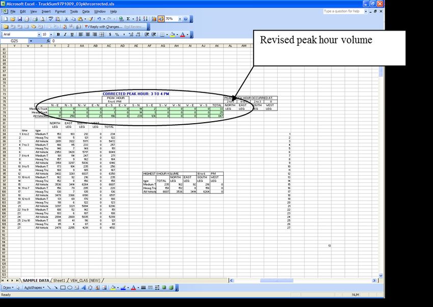
ACKNOWLEDGEMENTS

The following individuals were contributors in the preparation of this manual.

Oregon Department of Transportation

Kent Belleque, P.E.
Alexander Bettinardi, P.E.
Rod Cathcart
Don Crownover, P.E.
Brian Dunn, P.E.
Simon Eng, P.E.
Christina Fera-Thomas
Meghan Hamilton
Mark Johnson, P.E.
Chi Mai, P.E.
Christina McDaniel-Wilson
Joseph Meek III, P.E.
Nancy Murphy
Thanh Nguyen, P.E.
Douglas Norval, P.E.
Robert Nova
Gary Obery, P.E.
Peter Schuytema, P.E.
Dorothy Upton, P.E.

DKS Associates, Inc.

John Bosket, P.E.
Carl Springer, P.E.
Bob Schulte

CH2M Hill

Craig Grandstrom, P.E.

Copyright @ 2006 by the Oregon Department of Transportation. Permission is given to quote
and reproduce parts of this document if credit is given to the source. This project was funded in
part by the Federal Highway Administration, U.S. Department of Transportation.

The contents of this report reflect the views of the Oregon Department of Transportation,
Transportation Planning Analysis Unit, which is responsible for the facts and accuracy of the
information presented herein. The contents do not necessarily reflect the official views or
policies of the Federal Highway Administration.

Analysis Procedure Manual Version 1             ii                          Last Updated 11/2018
This manual is provided to you by the Oregon Department of Transportation (ODOT) "as is"
without warranty of any kind. ODOT makes no warranties, either express or implied, including,
but not limited to the implied warranties of merchantability, fitness for a particular purpose, and
noninfringement. The entire risk as to the quality and performance of this information is with
you. You are advised to test use of the information thoroughly before you rely on it. The author
and ODOT disclaim all liability for direct, indirect or consequential damages, arising out of your
use of the manual.

Analysis Procedure Manual Version 1             iii                          Last Updated 11/2018
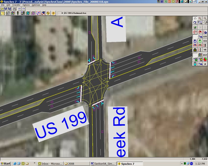
Table of Contents

1   INTRODUCTION – SEE APM VERSION 2 PREFACE AND CHAPTER 1 ............................ 1-1

2   MANAGING ANALYSIS PROJECTS – SEE APM VERSION 2 CHAPTER 2 ........................ 2-1

3   TRANSPORTATION SYSTEM INVENTORY - SEE APM VERSION 2 CHAPTER 3 .......... 3-1

4   DEVELOPING DESIGN HOUR VOLUMES - SEE APM VERSION 2 CHAPTERS 5 AND 6 4-
1

5   ASSESSING PERFORMANCE....................................................................................................... 5-1

    5.1     PURPOSE – SEE APM VERSION 2 CHAPTER 4 .................................................... 5-1
    5.2     CRASH ANALYSIS - SEE APM VERSION 2 CHAPTER 4....................................... 5-1
    5.3.    PEAK HOUR FACTORS – SEE APM VERSION 2 CHAPTER 5 .............................. 5-1
    5.4     ACCESS MANAGEMENT- SEE APM VERSION 2 CHAPTER 4 .............................. 5-1
    5.5     SIGHT DISTANCE- SEE APM VERSION 2 CHAPTER 4 ........................................ 5-1
    5.6     MULTI-MODAL ANALYSIS - SEE APM VERSION 2 CHAPTER 14 ...................... 5-1
    5.7     OTHER ANALYSIS ISSUES/PROCEDURES – SEE APM VERSION 2 PREFACE ..... 5-1

6   SEGMENT ANALYSIS– SEE APM VERSION 2 CHAPTER 11................................................ 6-1

7   INTERSECTION ANALYSIS – SEE APM VERSION 2 CHAPTERS 12 AND 13 ................... 7-1

8   TRAFFIC SIMULATION MODELS .............................................................................................. 8-1

    8.1     PURPOSE ...................................................................................................................... 8-1
    8.2     TRAFFIC SIMULATION MODELING – GENERAL CALIBRATION INSTRUCTIONS ........ 8-1
    8.3     SIMTRAFFIC ................................................................................................................ 8-4
          8.3.1      OVERVIEW ......................................................................................................... 8-4
          8.3.2      SIMULATION CALIBRATION................................................................................ 8-4
          8.3.3      SIMULATION PREPARATION ............................................................................... 8-5
          8.3.4      SIMULATION SETTINGS WINDOW ....................................................................... 8-6
          8.3.5      SIMTRAFFIC PARAMETER FILE........................................................................... 8-9
          8.3.6      SIMULATION EXECUTION ................................................................................. 8-12
          8.3.7      SIMULATION OUTPUTS ..................................................................................... 8-13

Analysis Procedure Manual Version 1                                iv                                       Last Updated 11/2018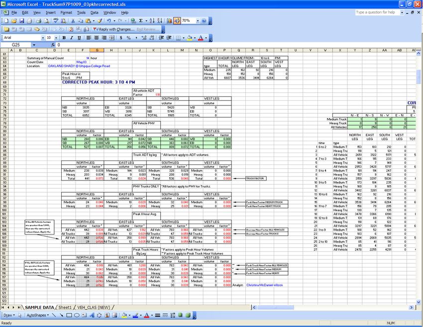
8.4      VISSIM - OVERVIEW.................................................................................................... 8-1
     8.5      PARAMICS - OVERVIEW .............................................................................................. 8-2
     8.6      CORSIM - OVERVIEW ............................................................................................... 8-3

9    DETERMINING NEEDS – SEE APM VERSION 2 CHAPTER 9 .............................................. 9-1

10         ANALYZING ALTERNATIVES – SEE APM VERSION 2 CHAPTER 10 ...................... 10-1

11         AIR AND NOISE TRAFFIC DATA ....................................................................................... 11-1

     11.1 PURPOSE .................................................................................................................... 11-1
     11.2 INPUT FOR NOISE ANALYSIS ..................................................................................... 11-1
           11.2.1      COMMON DATA NEEDS.................................................................................... 11-1
           11.2.2      CALCULATIONS ................................................................................................ 11-3
           11.2.3      PROCESS ........................................................................................................ 11-13
     11.3 INPUT FOR AIR QUALITY ANALYSIS....................................................................... 11-13
     11.4 EISBASE .................................................................................................................. 11-13
           11.4.1      OUTPUT AND FINAL PRODUCT ....................................................................... 11-15

12         TRAFFIC ANALYSIS REPORTS .......................................................................................... 12-1

     12.1 PURPOSE .................................................................................................................... 12-1
     12.2 BACKGROUND ........................................................................................................... 12-1
           12.2.1      TECHNICAL WRITING TIPS ............................................................................... 12-1
           12.2.2      DIAGRAMS AND ILLUSTRATIONS ...................................................................... 12-2
           12.2.3      TABLES ............................................................................................................ 12-3
     12.3 TECHNICAL MEMORANDUM ..................................................................................... 12-3
           12.3.1      PURPOSE .......................................................................................................... 12-3
           12.3.2      PRODUCTS........................................................................................................ 12-3
           12.3.3      DISTRIBUTION .................................................................................................. 12-4
     12.4 TRAFFIC NARRATIVE REPORT ................................................................................. 12-4
           12.4.1      PURPOSE .......................................................................................................... 12-4
           12.4.2      PRODUCT ......................................................................................................... 12-4
           12.4.3      DISTRIBUTION .................................................................................................. 12-7

Analysis Procedure Manual Version 1                                  v                                       Last Updated 11/2018
Table of Exhibits

Exhibit 8-1 Simulation Construction and Application Flow Chart ............................................. 8-3
Exhibit 8-2 Example Vehicles Exited from Performance Report ................................................ 8-5
Exhibit 8-3 Default Lane Alignment ........................................................................................... 8-7
Exhibit 8-4 Headway Factors....................................................................................................... 8-8
Exhibit 8-5 SimTraffic Default Vehicle Parameters .................................................................. 8-10
Exhibit 8-6 SimTraffic Default Driver Parameters .................................................................... 8-11
Exhibit 8-7 ODOT Green React Times ..................................................................................... 8-11
Exhibit 8-8 ODOT Intervals Defaults ........................................................................................ 8-12
Exhibit 8-9 Sample Queuing and Blocking Report ................................................................... 8-15
Exhibit 8-10 Sample Queuing Diagram ..................................................................................... 8-16
Exhibit 8-11 Sample Performance Report ................................................................................. 8-17
Exhibit 8-12 Sample Arterial report .......................................................................................... 8-17
Exhibit 8-13 Animated Vehicle and Signal Tracking ................................................................ 8-18
Exhibit 8-14 Example Queue Length Static Report .................................................................... 8-1
Exhibit 11-1 Sample Link Diagram – Jackson School Road Interchange ................................. 11-2
Exhibit 11-2 TruckSum Input .................................................................................................... 11-7
Exhibit 11-3 TruckSum Output ................................................................................................. 11-8
Exhibit 11-4 EISBase Input Screen (Replacement pending.) .................................................. 11-14
Exhibit 11-5 Traffic Analysis Output for Noise Analysis (Replacement pending.) ................ 11-16

Analysis Procedure Manual Version 1                              vi                                    Last Updated 11/2018
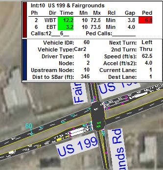
Table of Examples

Example 11-1 ........................................................................................................................... 11-15

Analysis Procedure Manual Version 1                                  vii                                     Last Updated 11/2018
1 INTRODUCTION – SEE APM VERSION 2 PREFACE AND
  CHAPTER 1

Analysis Procedure Manual Version 1   1-1   Last Updated 11/2018
2 MANAGING ANALYSIS PROJECTS – SEE APM VERSION 2
  CHAPTER 2

Analysis Procedure Manual Version 1   2-1   Last Updated 11/2018
3 TRANSPORTATION SYSTEM INVENTORY - SEE APM
  VERSION 2 CHAPTER 3

Analysis Procedure Manual Version 1   3-1   Last Updated 11/2018
4 DEVELOPING DESIGN HOUR VOLUMES - SEE APM
  VERSION 2 CHAPTERS 5 AND 6

Analysis Procedure Manual Version 1   4-1   Last Updated 11/2018
5 ASSESSING PERFORMANCE

5.1   Purpose – SEE APM VERSION 2 CHAPTER 4
5.2   Crash Analysis - SEE APM VERSION 2 CHAPTER 4
5.3. Peak Hour Factors – SEE APM VERSION 2 CHAPTER 5
5.4   Access Management- SEE APM VERSION 2 CHAPTER 4
5.5   Sight Distance- SEE APM VERSION 2 CHAPTER 4
5.6   Multi-Modal Analysis - SEE APM VERSION 2 CHAPTER 14
5.7   Other Analysis Issues/Procedures – SEE APM VERSION 2 PREFACE

Analysis Procedure Manual Version 1   5-1                 Last Updated 11/2018
6 SEGMENT ANALYSIS– SEE APM VERSION 2 CHAPTER 11

Analysis Procedure Manual Version 1   6-1   Last Updated 11/2018
7 INTERSECTION ANALYSIS – SEE APM VERSION 2
  CHAPTERS 12 AND 13

Analysis Procedure Manual Version 1   7-1   Last Updated 11/2018
8 TRAFFIC SIMULATION MODELS
8.1 Purpose
Traffic simulation models are complex tools that can provide valuable information on the
performance and potential improvement of transportation systems. Traffic simulation models are
in a constant state of improvement and accordingly this chapter attempts to be adaptive with the
changes in the industry. This chapter currently presents instruction on calibration of
microsimulation models created in Trafficware’s SimTraffic and a brief overview of the other
simulation models and parameters used in ODOT projects. Topics covered include:
Traffic Simulation Modeling – General Calibration Instructions
SimTraffic – Overview and Calibration Instructions
VISSIM – Overview
Paramics - Overview
CORSIM – Overview
8.2 Traffic Simulation Modeling – General Calibration Instructions
Traffic simulation models are computer programs that simulate traffic movements over a user-
defined transportation network and present the results via animation and reports. The degree of
user control over the simulation and the types of facilities that can be modeled will vary
depending on the program being used. These should not be confused with urban travel demand
models (Chapter 6), which use current and projected land use and transportation network data to
estimate current and future travel demand and traffic patterns.
Traffic simulation models (meso or microscopic) are complex tools that generally require more
labor than programs that perform capacity analysis at a macro level. Because of this, they are
generally only used when the use of other types of analysis tools will not be adequate for a given
project. Simulation models offer a greater degree of flexibility than most programs designed
specifically for capacity analysis and can be used for a wide range of analysis needs such as
examining the interactions between different modes of transportation, modeling the operations of
HOV lanes or bus priority systems and evaluating operations through measures of effectiveness
not offered by most other types of analysis programs. Simulation models are also very useful for
presentations, especially for those given to audiences lacking technical knowledge of traffic
analysis, because it provides a visual basis for evaluating operations that most people can easily
relate to and understand.
Simulation models are commonly used by ODOT to analyze corridors or networks under
congested conditions, where upstream or downstream operations have a significant influence on
actual intersection operations (e.g., intersection blockage from queue spillback). It should be
noted that simulation models use different methodologies for estimating queue lengths than other
procedures described in this manual. These methodologies are typically based on observations of
queues experienced during simulation, which are influenced by parameters such as driver
characteristics, lane changing behavior and various traffic flow interactions. Capturing the
impact of up and downstream operations on vehicle queues can make these models very effective
at estimating queue lengths, but underscores the importance of good model calibration. General
Analysis Procedure Manual Version 1 8-1 Last Updated 11/2018guidelines for the application of simulation models have been published by the Federal Highway Administration, which can be found at the FHWA website under traffic analysis tools. Depending on the specific program used, there may be numerous parameters that can be manipulated by the user to create a system that most accurately represents the one being analyzed. Before any simulation model is used to represent existing or future conditions, the existing conditions model created must be calibrated by adjusting operational parameters until the model provides a reasonable representation of existing conditions measured in the field. Existing conditions need to be replicated; otherwise future conditions will not be correct. Existing conditions should include only data, operations and measures known to currently exist in the project study area. Vehicle counts should be kept as close as possible to the original volumes obtained from the field. If all counts are available from the same day, vehicle counts used during calibration should be un-factored and unbalanced counts (this day should be as close to the 30th highest hour as possible). If counts cannot all be collected on the same day (or year), every effort should be made to collect counts at primary locations on a day that is on or closely represents, the 30th highest hour. The remaining counts can then be factored and balanced to this primary count day. If all counts occur on scattered days and none of the counts occur on the 30th highest hour or on a representative day then short sample count should be conducted to factor the off- peak counts to the day the study area was visited. Use the seasonal factor methodology described in Chapter 5 to determine if the count is close enough to the 30th highest hour. If the primary counts for the study area occurred during a time that is less than 90% of the 30th highest hour for that area seasonal trend type, then a re-visit with a sample count is required for the calibration of the “existing” model. These rules are established to help ensure that calibration volumes 1) are near the 30th highest hour and 2) represent conditions that have been witnessed in the field. The emphasis is placed on witnessed, as the analyst needs to visit the study area on or near the count day (30th highest hour) so that the visual check of the simulation (the first step in calibration) is based on conditions that occurred in the field during the count. The Field Inventory Worksheet shows all the measures from the field that should be input into the simulation and visually checked in the animation to help analysts in the data collection process. Chapter 3, Transportation System Inventory, shows an example completed worksheet for a simulation project. Note that the worksheet is intended to be printed multiple times for a given project area. The collection of worksheets can be placed in a three-ring binder providing a hard writing surface. Each copy of the worksheet can be used for each intersection or area of interest in the study and all copies can be neatly organized in a single project binder (see Chapter 3). The site visit should occur as close as possible to the 30th highest hour. After the site a calibration scenario can be constructed. For the purpose of calibration, the peak hour volumes from the counts should be seasonally adjusted to the time period of the site visit. The calibration network should include all measurements taken and all operational behavior witnessed. Many of the behavioral issues should be collected on the worksheet provided above. For Synchro and SimTraffic inputs refer to Chapters 12 and 13. Some of these sections refer specifically to Synchro/SimTraffic, but the list provided should include most of the measures that would have to be checked or adjusted in any software platform. Note that most microsimulations go into greater detail than SimTraffic, so there will likely be more measures to check and adjust. Also note that illegal behavior such as speeding, improperly using medians or shoulders as turn bays Analysis Procedure Manual Version 1 8-2 Last Updated 11/2018
and improper lane changing distances should be accounted for in during calibration, but should
not be continued to be assumed in the future build scenarios. All non-calibration alternative
analysis should assume that all drivers follow the rules of the road.

Once the “existing” inputs and behavior is coded into the simulation software, the analyst should
run an animation to visually check the reasonability of the microsimulation. Any gross error like
queues or blockages being much greater or much less than the field observations should be
addressed by re-checking inputs. Further refinement may include measuring and adjusting
saturation flow rates, driver reaction time and travel speed. A good place to start is by comparing
simulated vehicle queues to those visually observed in the field. For some corridors, comparing
simulated travel times or average speeds to actual observed conditions may be appropriate.

Good calibration is not only critical for accurate analysis, but will establish credibility during
presentations with technical advisory committees or public groups that have prior knowledge of
existing problem areas. Exhibit 8-1 illustrates how the calibration process fits into the complete
analysis. The calibration, existing and site visit hour refer to the same hour. In other words, the
“calibration” data is collected in the study area in the “site visit” hour to represent “existing”
conditions. For further information on calibration in general, consult the FHWA Analysis
Toolbox. Section 8.3 has the detailed procedures on calibrating a SimTraffic model using
SimTraffic for ODOT projects.

Exhibit 8-1 Simulation Construction and Application Flow Chart

                                                      Raw Counts
                                                   Annual Adjustments
                                       If needed
                                                    Seasonal Factors

   Field Measurements: Headway,
                                                    Calibration Hour
                 Free-Flow Speed
                                                    “Existing” Hour
            Engineering Judgment
                                                     Visit Site Hour
       Calibrated Using “Vehicles
           Exited” for SimTraffic

    Likely to be       Annual Adjustments           30th Highest Hour
        needed            Seasonal Factors               Volumes

                                                                     Annual Adjustments
                                                                 Future Path Adjustments

                       May need to bring
                     headway factors and
                                                    Build or Analysis
                     posted speed back to
                                                     Year Volumes
                   defaults – Engineering
                                Judgment

Analysis Procedure Manual Version 1                  8-3                    Last Updated 11/2018
8.3 SimTraffic 8.3.1 Overview SimTraffic performs microsimulation and animation of vehicle traffic, modeling travel through signalized and unsignalized intersections and arterial networks, as well as freeway sections, with cars, trucks, pedestrians and buses. SimTraffic includes the vehicle and driver performance characteristics developed by the Federal Highway Administration for use in traffic modeling. They were developed for CORSIM and Trafficware used them as they were published. Most of the input is entered through the Synchro program, but some parameters, such as the driver and vehicle characteristics, are modified through SimTraffic specifically. SimTraffic can be used for all ODOT plans, projects and traffic impact studies. SimTraffic is primarily used by ODOT for the analysis of signal systems and vehicle queue estimation, especially in congested areas and locations where queue spillback may be a problem. For the estimation of signalized vehicle queues, SimTraffic is generally preferred in Regions 2 through 5 where v/c ratios exceed 0.70 and in Region 1 where v/c ratios exceed 0.90, but should always be used where v/c ratios exceed 0.90. SimTraffic should typically be used for the analysis of all coordinated signal systems. For isolated intersections, Synchro and SimTraffic should provide similar results. SimTraffic results will differ from Synchro most when the v/c ratio exceeds 0.90, when there are closely spaced intersections and other conditions that are not ideal. Overcapacity queues and metering conditions are identified in Synchro’s Timing Window with a “#” or “m” symbol. 8.3.2 Simulation Calibration As much as possible, operational field data should be obtained for the major facilities in the study area as close as possible to the design hour (see Appendix H). Beyond the field data listed in Chapter 3, additional field measures may be needed to achieve calibration of the microsimulation. If needed, saturation flow studies should be performed at the major intersections. Floating car travel time runs may need to be performed to ensure that observed and simulated travel times (and related speeds) are close. Free-flow link speeds using road-tube counters or speed guns (RADAR, LIDAR, etc) may need to be collected and used in place of posted speed limits during calibration. At the very least, the existing conditions network needs to be visually calibrated to the field conditions and the “vehicles exited” measure from SimTraffic should be reviewed. If everything is close, then the SimTraffic simulation should duplicate conditions seen in the field. Congested and free-flow areas in the field should be congested and free-flowing in the simulation. If there is more congestion in the simulation than in the field, then one or more parameters may be off. For example, saturation flows and resulting headway factors may be too low, counts may be balanced too high, peak hour factors may be too low, link and turning speeds may be low, storage bays and taper lengths may be too short and intersection paths and lane change distances may be incorrect. If congestion is too low then the reverse of these may be a cause. To help determine the cause of inconsistencies with known conditions, any number of measures Analysis Procedure Manual Version 1 8-4 Last Updated 11/2018
of effectiveness (MOE) may be reviewed, however as a minimum measure, “ vehicles exited”
needs to be checked to ensure that the model is calibrated.

“Vehicles Exited” represents the number of vehicles that make it through an intersection over a
given period of time. This should equal the volume coded in the network for the “existing hour”.
The calibration target for each intersection in the network is a tolerance of 1% over the analysis
period based on the difference between the simulation and the input field-counted exiting
(existing) hour volumes. However, at a minimum, the tolerances for any movement over 100 vph
should be within 5% of the coded volume. Movements with less than 100 vph should be checked
to make sure that the vehicles exiting is reasonable. These limits are required to achieve
calibration for the calibration volume set (not required for the 30th highest hour or build year
network). Exhibit 8-2 shows an excerpt from the Performance report showing the Vehicle Exited
rates and calibration percentages. Note that all movements over 100 vph are under the 5%
maximum tolerance and the entire intersection is under the 1% intersection tolerance.

Exhibit 8-2 Example Vehicles Exited from Performance Report

Although calibration (fine-tuning) may take some time, it is necessary because if the existing
conditions is not duplicating observed conditions, then the future conditions or build alternative
performance will not be predicted very well. This is critical if any animated output is to be
shown at public meetings. In achieving accurate calibration it is important that the SimTraffic
parameter file is setup properly.

8.3.3 Simulation Preparation

In addition to setting up the SimTraffic parameter file, there are a number of Synchro settings
that must be updated for simulations to work properly in SimTraffic. More signal timing detail
must be added in the Phasing Window. These phasing details, settings and defaults are shown in
Chapters 12 and 13. Project data needs to be entered into the Simulation Settings Window and
the Detector Window. The Detector Window is covered under the Synchro sections in Chapter
13 because detector data is necessary if actuated signal functions are to be used in Synchro. The
important Simulation Settings Window and the SimTraffic parameter data are included in
Section 8.3.3 and 8.3.4, respectively. Earlier versions of SimTraffic only need to create the
SimTraffic parameter file.

Analysis Procedure Manual Version 1             8-5                  Last Updated 11/2018
8.3.4 Simulation Settings Window
The following data is only used by SimTraffic and needs to be included for a proper simulation.
This data allows for geometric refinement and operational behavior of the simulation. The data
required by SimTraffic should be a part of the field collection/observation process and is
included the Field Inventory Worksheet.
Storage Length (ft) – The Storage Length is the length of a turning bay from the stop bar
to the beginning of the taper. Storage Length is the area that can store vehicles and does
not include tapers. If the Left or Right Turn lane goes all the way back to the previous
intersection, enter "0". Storage Length data is used for analyzing potential blocking
problems. Storage length is typically field measured or estimated from aerial
photographs. If measurements are unknown or if the facility is new, the initial storage
lengths of 100’ for urban and 150’ for rural can be used. SimTraffic outputs will be used
to refine these lengths for build alternatives.
Taper Length (ft) – The Taper Length is the remaining length of the turning bay from
the end of the storage length to where the outer edge of the turning bay meets the outer
edge of the adjacent lane. This value is field-measured or estimated from aerial
photographs. For state highways, the taper lengths can be obtained from the Highway
Design Manual Figures 8-8 for right turn lanes and 8-9 for left turn lanes. This allows
turning bays to store several more vehicles and allows a truer and a more consistent (with
design) representation.
Lane Alignment – The Lane alignment controls the vehicle paths in SimTraffic. When
links are constructed, Synchro shows either a “Left” or “Right” alignment as default. This
may not be correct especially if multilane approaches, skewed intersections, short links,
free-flow ramp connections and merge/diverge/weaving sections make up a particular
intersection.
Other choices are “L-NA” and “R-NA” which will force the vehicle path either left or
right. To check the lane alignment, the Intersection Paths box must be checked under the
Map Settings window. The default color or zoom level will likely need to be changed to
clearly see the paths.
Exhibit 8-3 shows that Synchro defaults to single-lane turn lanes turning into a multilane
leg with paths going to either departing lane. Unless lines are marked on the pavement
guiding vehicles into different lanes Oregon vehicular code states that vehicles need to
turn into the nearest lane. In most of these cases the Lane Alignment needs to be changed
to “L-NA” or “R-NA” depending on the turn type.
Analysis Procedure Manual Version 1 8-6 Last Updated 11/2018Exhibit 8-3 Default Lane Alignment
For the existing calibrated network, the legal setting may not need to be followed if the
majority of field-observed vehicles turn into both lanes (although itself an improper lane
choice). Design alternatives should be always be coded legally.
Note that the northbound dual left turn lane shown in Exhibit 8-3 has the correct paths.
The southbound left still needs to be changed to limit traffic to the inside through lane. In
cases of acceleration lanes, merging traffic should be forced right using “R-NA” and
through traffic forced left using “L-NA.” This will keep through vehicles out of the
acceleration lane.
Enter Blocked Intersection – This setting controls whether mainline or side-street
traffic can enter a blocked intersection. In earlier versions of SimTraffic, vehicles did not
block intersections. Default is “No” for intersections and “Yes” for bend nodes and ramp
junctions. This factor is best obtained through field observation.
Along many busy roadways, minor intersections and driveways are frequently blocked by
through traffic, so in this case the setting should be “Yes” for the through traffic. If “Do
Not Block Intersection” signs exist, then the setting should remain “No” unless the signs
are generally ignored. If there are intersections or accesses that are frequently blocked
and through vehicles let side street vehicles out, then the side street movements can be set
to “1 veh” which will allow one vehicle to enter. Use of the “2 veh” setting has a
tendency to cause the simulation to clog up.
Link Offset (ft) – The Link Offset is used to set the roadway left or right of the natural
centerline. This is typically used in creating “dogleg” or offset intersections without
Analysis Procedure Manual Version 1 8-7 Last Updated 11/2018creating a second node.
Crosswalk Width (ft) - this is the width of the crosswalk on an approach. This setting
controls the placement of the stop bar which controls detector placement and link length.
ODOT default crosswalk width is 12 feet (outside edge to outside edge) unless the
adjoining sidewalk is wider. Local intersections should be measured.
Headway Factor - The saturation flow rate in SimTraffic for intersection approaches is
adjusted through the Headway Factor. The saturated flow rate calculated in Synchro is
not used in SimTraffic; however, the corresponding headway factor is automatically
calculated. In simulation calibration, the headway factor can be adjusted to help fine-tune
(calibrate) the SimTraffic simulation. Exhibit 8-4 shows the equivalent headway factor
for a given saturated flow rate. Earlier versions of Synchro/SimTraffic need to have the
headway factor manually calculated in the Lane Window.
Exhibit 8-4 Headway Factors
Headway Factor Saturated Flow Rate
1.2 1650 vphpl
1.1 1750 vphpl
1.0 1850 vphpl
0.9 2050 vphpl
0.8 2250 vphpl
Turning Speed (mph) – This is the turning speed used by SimTraffic by movement.
Higher speeds will increase the capacity of the SimTraffic simulation. Synchro default is
15 mph for left turns and 9 mph for right turns. The 9 mph right turn speed is too slow
unless used for turning onto residential local streets or in a downtown central business
district location.
ODOT default is 15 mph for left and right turns. Non-standard turns at skewed
intersections, channelized turns and interchanges should have different values and can be
estimated by recording speeds while driving through the subject intersections or using a
speed gun to capture turning vehicle speeds. Turning speeds are also needed for
merge/diverge sections at interchanges or bend nodes.
Lane Change Distances - Changes to these calculated values can help calibrate the
vehicle lane-changing operation. Changes may be necessary if vehicles are having
difficulty completing lane changes ahead of intersections or off-ramps or if vehicles are
artificially clogging up at lane drops after an intersection or a two-lane ramp merging into
a single lane. High heavy vehicle percentages combined with a higher amount of long
vehicles and/or a congested network increases the chances that modifications will be
required. Closely spaced intersections will have short lane change distances while
interchanges will have longer lane change distances as many drivers move into the
desired lane considerably ahead of an off-ramp. The analyst will need to experiment with
these values, either longer or shorter until the traffic is flowing consistent to the observed
conditions or flowing smoothly for future conditions. Modifying ramp geometry so that
the ramps enter the mainline as turns rather than as a straight-through movement makes
for smoother operation and less need to modify these distances.
Analysis Procedure Manual Version 1 8-8 Last Updated 11/2018There are two different types of lane change distances: mandatory and positioning. The
Mandatory Distance is the distance measured from the stop bar at which a lane change
must occur. The Positioning distance is the distance measured back from the Mandatory
Distance where a vehicle first attempts a lane change. The Mandatory and Position
Distance 2’s are extra distance added if a second lane change is necessary. All of these
distances can extend around corners. Adding to the challenge of changing these variables,
is that the driver types in SimTraffic have a range of a 50% (aggressive) to a 200%
(passive) multiplier to the set distances.
8.3.5 SimTraffic Parameter File
The SimTraffic parameter file controls the simulation operation and the defaults must be
changed to reflect the proper impacts of queuing, travel time, etc. The parameter file has three
major sections: Vehicles, Drivers and Intervals. The TPAU Analysis Tools webpage has a
default SimTraffic template file with all of the basic parameters set up. The following shows the
variables that need to be changed. All other settings are left unchanged.
The Vehicles tab controls the type and physical vehicle characteristics.
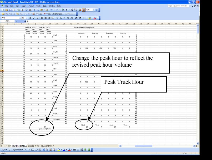
Vehicle Occurrence (%) - SimTraffic uses the Synchro heavy vehicle percentage to
simulate the total number of heavy vehicles relative to all vehicles. When the simulation
calls for a heavy vehicle, the vehicle type is represented by this factor which represents
the percentage breakout of the global truck fleet. Likewise, when a car is called for, this
factor will split the car types among the global car fleet percentages.
o Earlier versions of SimTraffic defaulted to having the total vehicle percentages
sum up to 100%.
o SimTraffic 7 defaults total up to 100% for the car fleet and 100% for the truck
(includes buses) fleet as shown in Exhibit 8-5.
o Change the Vehicle Occurrence (%) for the different vehicle classes to match the
composite average of your classification counts. If classification counts are
unavailable, state highway vehicle classification segment data (available at
https://highway.odot.state.or.us/cf/highwayreports/traffic_parms.cfm) can be used
substituted. Average between multiple counts at the project boundaries and on
different significant facilities both state and local. Note that while the heavy
vehicle percentages per approach may vary largely, the heavy vehicle mix does
not vary as much. The total truck fleet should total up to 100% and the total car
fleet should total up to 100%.
Car1 represents the larger passenger vehicles in the fleet (i.e. SUV’s, large
pickups);
Car2 represents smaller passenger vehicles in the fleet;
TruckSU represents single unit trucks (i.e. delivery vans, dump trucks);
SemiTrk1 represents single tractor-trailer combinations;
SemiTrk2 represents shorter single tractor-trailer combinations;
Truck DB represents trucks with two trailers; Note: SemiTrk2 and Truck
DB can be customized to fit other truck types like triple trailers.
Bus represents buses in the fleet;
Carpool1 & Carpool2 represents vehicles with the same characteristics as
Car1 and 2 but with higher occupancies. Zero out the default Carpool1 and
Analysis Procedure Manual Version 1 8-9 Last Updated 11/2018Carpool2 vehicles. These will have no effect on the simulation unless
vehicle occupancy is used as an evaluation measure.
Exhibit 8-5 SimTraffic Default Vehicle Parameters
These percentages should reflect the relative
differences between vehicle classes in the
manual counts.
Vehicle Length (ft) – This parameter directly affects queuing distances. Leaving the
length unchanged will result in the queues being underestimated. Change the vehicle
length in the following vehicle types:
o Car1 = 20 ft;
o Car2 = 16 ft;
o TruckSU = 30 ft;
o SemiTrk1 = 75 ft.
The Drivers tab (Exhibit 8-6) controls the behavior characteristics for the 10 different driver
types that make up the simulation from the passive to the aggressive. For example, Driver Type 1
has 15% lower link speeds and will take 200% more distance when making a lane change while
Driver Type 10 will travel 15% faster than the link speed and have lane change distances 50% of
the coded values. All of the factors in the Drivers tab remain the same with exception of the
Green React (s) setting. This setting reflects the time from when the signal turns green to the
time that the vehicle begins to move. This value can be captured in the field and used as a
calibration parameter. TPAU research indicates that Oregon values are substantially different
than the defaults in SimTraffic. Change the Green React times to match Exhibit 8-7.
Analysis Procedure Manual Version 1 8-10 Last Updated 11/2018Exhibit 8-6 SimTraffic Default Driver Parameters
Exhibit 8-7 ODOT Green React Times
Driver
Type 1 2 3 4 5 6 7 8 9 10
Green
React 2.0 1.6 1.3 1.1 1.0 0.9 0.9 0.8 0.7 0.5
(s)
The Intervals tab controls the actual operation and data recording of the simulation. Exhibit 8-8
shows the ODOT interval defaults.
Seeding “0” Interval – The Seeding Interval fills the network before any statistics are
recorded. This value must be long enough for vehicles to travel the length of the network.
ODOT default is 10 minutes or the time to travel the longest trip on the network,
whichever is longer.
Recording Intervals – Simulation statistics are recorded in these intervals. The ODOT
default uses at least two intervals, one 15-minute in length to represent the peak 15-
minute period and one 45-minute interval to fill out the hour simulation period. However,
you can have more intervals if you would like. For future analysis networks, the 15-
minute interval is preferably placed as the first recording interval because it most
represents the peaking in the output reports, regardless of where it occurs in the actual
peak hour. However, for the calibration network, the 15-minute peak period should be
coded to represent the actual peak 15-minute period as it occurred during the counts. The
names of the recording intervals can be anything as they have no impact on the results.
Duration (min) – Change to 10 minutes (time to cross the network if longer) for the
seeding interval, 15 minutes for the first recording interval and 45 minutes for the second
recording interval (or, if this is being applied to the calibration work, a distribution
representing the peak as it occurred in the counts).
Analysis Procedure Manual Version 1 8-11 Last Updated 11/2018 Start Time (hhmm) – After Duration is specified, change the start time to reflect the
hour being simulated.
Record Statistics – Set to “Yes” for all recording intervals.
Growth Factor Adjust – Set to “Yes” for all intervals.
PHF Adjust & AntiPHF Adjust – The combination of these two settings creates a spike
in the simulated hour. The PHF Adjust should be set to “Yes” during the seeding and the
peak 15-minute intervals and the AntiPHF Adjust set to “No.”. The AntiPHF Adjust
should be set to “Yes” and the PHF Adjust set to “No” for all other recording intervals.
Percentile Adjust - Set to “No” for all intervals. Use of this setting will overestimate the
queuing in the simulation.
Random Number Seed – SimTraffic uses nine different simulation scenarios (1 through
9). If it is desired to produce duplicate results, select a non-zero setting. ODOT default is
to set it to ‘0’ which will produce random arrival rates with each run.
Exhibit 8-8 ODOT Intervals Defaults
8.3.6 Simulation Execution
Once all Synchro and SimTraffic settings are completed, the simulation is ready to be executed.
Upon starting the simulation, the “Errors and Warnings” window will appear. This shows
anything that is outside of the value ranges what SimTraffic expects to find. Errors are split into
fatal and non-fatal errors. Fatal errors will not allow the simulation to run and must be corrected.
Fatal errors usually are related to lanes and lane groups where no lanes exist on a link.
Non-fatal errors still allow a simulation to be run, but these need to be reviewed and corrected if
possible for best results. Some examples of non-fatal errors that need to be corrected are:
“Detector too close to stop bar” ;
Minimum green /total split/pedestrian timing errors;
Analysis Procedure Manual Version 1 8-12 Last Updated 11/2018 Reference phase not in use errors;
Storage lane and length errors.
Some examples of non-fatal errors that can be left alone as these are “how it is” are:
“Angle between approaches less than 25 degrees.” Small angles will lengthen out an
intersection area and may cause unpredictable operation.
Any error referencing vehicle extensions or minimum gaps exceeding 111% of travel
time between detectors. Errors such as these indicate that actuated signal operation will
be not as efficient.
“Volume-delay operation not recommended with long detection zone.” SimTraffic has
issues generally with ODOT’s default phasing variables.
ODOT standard is to average together at least five (5) random acceptably working (no system
gridlock) runs. If you have a congested or a large network, it is advisable to have 7-10 runs to
allow for “blown” runs which are caused by system gridlock so there are at least five good runs
averaged together at the end. The system gridlock is typically caused by the improper actions of
simulated vehicles that end up getting stuck. If every run or a majority of runs have gridlock,
then the analyst should further refine the simulation settings, especially the headway factors,
blocked intersection and lane change distance parameters.
It can take 20-40 minutes a run (depending on network size, congestion level and computer
speed). Make sure you have adequate available storage. Each simulation file can be in excess of
1 GB. If you run out of space during a multiple recording session, SimTraffic will continue to
run, but the simulations will stop being recorded.
Once the runs are completed, check each simulation run by selecting each number in the drop-
down run number box to make sure it is free of any system gridlock errors and that the
simulation reflects what is expected. If there are bad runs, make note of the run number, so it
may be skipped in the report process.
8.3.7 Simulation Outputs
SimTraffic outputs are used for queue analysis, determination of storage lane lengths, travel
times and other evaluation criteria. Many times in the evaluation of alternatives the typical v/c
and LOS measures may have very small differences. It is common practice today to use
additional MOE’s to describe an operation of an alternative. These MOE’s can include travel
time, stopped delay, average speed and queue blocking. These are very useful in alternative
comparisons because lower travel times, delays and stops coupled with higher average speeds,
will indicate a more operationally efficient alternative.
Make sure before selecting any report to print or preview that a number is showing in the run
number box. Otherwise, a message appears from SimTraffic saying that it needs to record the
simulation again.
To preview a report, select the desired report(s) and make sure that the Multiple Runs box is
checked. Select the desired .hst files (skipping any bad runs). Reports are generally broken down
into sections by intersection and interval. The Summary of All Intervals section of the report is
Analysis Procedure Manual Version 1 8-13 Last Updated 11/2018where information is pulled from for analysis. Check to make sure that content, headers and
footers are correct before printing.
Simulation Summary Report – Used to check whether that the runs look to have similar
characteristics. Entering and exiting vehicles, total delay and total stops should be
relatively consistent between runs. This is a second check of the run adequacy (the first is
visual inspection). This report also gives system total MOE’s which can be used in
alternative comparisons.
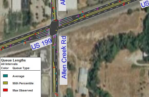
Queuing and Blocking Report - The Queuing and Blocking report generates the 95th
percentile queues which are used to design turn bay storage as well as document
operation of the study area.
Exhibit 8-9 shows a typical report.
This report shows three different queues: maximum, average and 95th. The reported
maximum queue is the highest queue calculated every two minutes. The average queue
(50th percentile) is the average of the calculated two-minute queues. The 95th Queue is the
95th percentile of the reported maximum queue over the simulated period. With the
Random Number Seed set to zero, the queues in this report will be different from those in
another set of simulation runs. When reporting out the estimated queue lengths, round up
to the next 25 feet.
Analysis Procedure Manual Version 1 8-14 Last Updated 11/2018Exhibit 8-9 Sample Queuing and Blocking Report
95th Percentile Queues
The Upstream Block Time and the Storage Block Time are of particular interest in helping
describe the overall impact of queuing. While the 95th percentile queues may show how long a
queue is, the block time shows for how long of the simulated hour the queue will block
intersections or storage bays.
Even if queue spillback into adjacent intersections is not occurring, storage bays may be
overflowing, causing local problems such as the blockage of adjacent lanes. A queue blockage or
spillback condition is considered a problem when the duration exceeds five (5) percent of the
peak hour. Spillback may also be a sign of cycle failure as there may not have been enough green
time available to serve all waiting vehicles. Signals do not recover instantly, so one spillback
cycle could affect the operation of the next two or three cycles which can be a significant portion
of hourly cycles.
Upstream Blk (Block) Time (%) - This is an estimated percentage of the peak hour in
which the queue from the subject node blocks an upstream node. This is especially useful
when analyzing a complex Synchro network, to determine the extent of queuing on a
system when reporting out results. It can also be used to determine if an alternative or
option will provide the best progression.
Storage Blk (Block) Time (%) - This reports an estimated percentage of the peak hour
Analysis Procedure Manual Version 1 8-15 Last Updated 11/2018in which the length of the through or turning queues exceeds the storage length. For build
analysis, if your storage block time is significant (>5%), then it is recommended to enter
a longer bay length, rerun the simulation and continue this until you get a percentage less
than 5%. Keep in mind that storage bays should adhere to the practical limit of 300 – 350
feet (most storage bays are 100 to 150 feet), so some alternatives and their simulations
will still have significant storage block time.
Queues can be reported directly from the subject approach if the queue length is less than the
link length. If a queue is longer than the link length, then the total actual queue length will be the
link length(s) that are completely filled up plus the last queue length that does not exceed the link
length. The analyst will need to trace the queue back from the intersection in question, so you
will likely pass though multiple intersections and bend nodes to obtain the actual queue length.
However, this queue is made up of contributions from other intersections that the subject queue
spills back into which can make it hard to tell and report where exactly the queue originates.
Queues are best reported graphically by identifying the queues under spillback conditions
separately from the ones that do not exceed the link length.
Exhibit 8-10 shows a sample 95th percentile queuing diagram. To minimize reporting issues, link
curvature should be used where possible to eliminate any unnecessary bend nodes.
The combination of the upstream and storage block times can also be used to report out the
impacts of queuing at a higher level instead of reporting out the 95th percentile queues for
intersection approaches.
Exhibit 8-10 Sample Queuing Diagram
I-5
NORTH
NO SCALE
N
.P
ho
en
ix
Rd
.
650’
OR
99 650’
375’
100’
Fern Valley Rd.
50’ 100’
275’ 550’ Luman Rd.
75’ 700’
325’ 175’
50’
150’
E. Bolz Ln.
. 200’
l Ln 100’ 250’
ery
Ch
S. Phoenix Rd.
950’
Lu
.
Ln
Pe
m
olz
an
ar
.B
Rd
Tr
W
ee
.
L
Be
n.
a rC
= Isolated 95th Percentile Queues re
ek
= Overlapping intersection 95th Percentile Queues
OREGON DEPARTMENT OF TRANSPORTATION TPAU TRANSPORTATION PLANNING ANALYSIS UNIT
File : Fern Valley.ppt Prepared By: C. Fera-Thomas
Fern Valley Interchange - 2004 30th Highest Hour No-Build 95th Percentile Queues
Date : 2/25/2005 Rev. By: P. Schuytema PE
FIGURE 3
Analysis Procedure Manual Version 1 8-16 Last Updated 11/2018 Performance Report - The Performance report (Exhibit 8-11) gives the MOE
comparisons for each intersection by approach, movement or run; for each approach by
run; or a total for the entire network. MOE’s are summed over the entire hour (i.e., hours
of delay). During calibration, “vehicles exited” needs to be used to ensure calibration, see
Section 8.3.1 for more instruction.
Exhibit 8-11 Sample Performance Report
Arterial Report – The Arterial Report (Exhibit 8-12) is another version of the
Performance report but reports out travel time, delay and speed along a roadway section
on a per vehicle basis. This roadway must have at least two nodes for this report to be
available for it and the roadway has to have the same road name without any special
characters (i.e. dashes) along all of the reported sections. The presence of a mixture of
one-way and two-way sections along an arterial corridor may require segmenting and the
individual results summed.
Exhibit 8-12 Sample Arterial report
Animated Tracking
In the SimTraffic simulation, clicking on a vehicle will bring up a box (Exhibit 8-13) showing
speed, acceleration, distance to next turn, etc. this will allow the analyst to track vehicles as they
travel through the network. Clicking on the vehicle again will remove the tracking box. In
addition, signalized intersections can be clicked on showing the signalized operation in action as
Analysis Procedure Manual Version 1 8-17 Last Updated 11/2018it goes through the phases. Both of these can be useful in debugging a simulation. It is recommended that the simulation speed be set to real time or slower for best viewing. Exhibit 8-13 Animated Vehicle and Signal Tracking Static Graphics Other reports include the “Static Graphics” reports (Exhibit 8-14). Select the Graphics tab and you will get a box showing reports such as total delay, percent time blocked queues, etc. These reports are based on the same information that the previous comprehensive reports use, but display the information in graphical form, rather than a table of numbers. These report out just the run number selected rather than an average of runs of the regular reports. These can be use to quickly visualize the issues for the analyst or for others. Analysis Procedure Manual Version 1 8-18 Last Updated 11/2018
Exhibit 8-14 Example Queue Length Static Report

8.4 Vissim - Overview
Vissim is a simulation program that can model multi-modal traffic flows including cars, trucks,
buses, heavy rail and light rail transit (LRT) as well as model traffic management systems (ramp
meters, toll roads, and special lanes) and transit priority systems. Vissim can also model trip
assignment, over fixed routes or dynamically, where vehicles change routes in response to
specified events and can animate traffic movements in 3-D. Vissim is a program that can stand
alone, but is data intensive to create files for use on its own. Alternatively, the files can be
created in Visum (a travel demand program) that can then import the files into Vissim for
analysis. See APM version 2 Appendix 8B for guidance on creating networks using PTV Vision
Suite software (Visum, Vissim, and Vistro). Because most ODOT region offices do not perform
travel demand modeling, it is important to note issues both with and without Visum.

Other advantages of Vissim include the rail-roadway interface, which requires Vissim Level 3 or
4 in order to model the effect of rail crossing blockages on queues and roadway operations.
Another advantage is that Vissim has the capability of “dynamic traffic assignment” (DTA),
which will reroute a vehicle on the network in case of a crossing blockage or an overcapacity
situation. Note that this strength of the software comes at the price of larger study areas to allow
for correct dynamic assignment and to address effects occurring potentially outside of the focus
of the study area. DTA will likely require more data, measures and resources to properly
calibrate (see APM version 2 Chapter 8 for more information).

Analysis Procedure Manual Version 1             8-1                  Last Updated 11/2018
APM version 2 Addendum 15A is a link to the ODOT Vissim Protocol which governs
documentation and creation of all Vissim models created for ODOT plans and projects.
Vissim has the capability of performing analysis directly on Visum traffic volume assignments
and includes a post-processing function. The results of this type of analysis may be acceptable
for certain applications, such as sketch planning and alternative screening. However, for most
types of analysis, DHVs are required. The function in Vissim does not create DHVs, therefore
the post-processing procedures outlined in APM version 2 Chapter 6 are still necessary.
Most ODOT region offices do not currently own the Vissim software (outside of Region 1). The
ODOT Synchro defaults should be implemented in the Vissim model to the extent possible. Most
region offices outside of Region 1 are unlikely to have the knowledge base to use Visum.
8.5 Paramics - Overview
Paramics and VISSIM share a lot of the same benefits in functionality and issues with
complexity and time to achieve calibration. Paramics, like VISSIM, is a simulation program that
can model multi-modal traffic flows including cars, trucks, buses, heavy rail and light rail transit
(LRT) as well as model traffic management systems (ramp meters, toll roads and special lanes)
and transit priority systems. Paramics can also model trip assignment, over fixed routes or
dynamically, where vehicles change routes in response to specified events and can animate
traffic movements in 3-D. Paramics is a program that can stand alone, but is data intensive to
create files for use on its own. Paramics does offer some importing functionality to bring
networks in from other software, but it does not have a direct link to VISUM. However, all of
Paramics’ inputs are text files, making it easy to customize automations (macros, scripts, etc.) to
take networks from other platforms and format the data into the text files Paramics requires. This
creates many opportunities to bring networks from any software quickly into Paramics.
Arguably the biggest strength of any dynamic assignment software (like Paramics and VISSIM)
is the “dynamic traffic assignment” (DTA) option, which will reroute a vehicle on the network in
case of a rail crossing blockage or an overcapacity situation. Note that this strength of the
software comes at the price of larger study areas to allow for correct dynamic assignment and to
address effects occurring potentially outside of the focus of the study area. DTA will likely
require more data, measures and resources to properly calibrate.
Paramics has disadvantages similar to VISSIM since it does not produce signal coordination
timing and can be very data intensive and time consuming to construct and calibrate a scenario,
especially from scratch.
Some issues to consider when using Paramics for analysis are (based on ODOT’s assessment of
version 5.2):
The flexibility of Paramics means the analyst is required, in most cases, to write their
own reports. Paramics does have a set of limited standardized reports. This would require
exporting the queuing data to Excel or comparable software; creating functions to
calculate the maximum queues for each time period, calculating averages and standard
deviations and then calculating the 95th percentile queue on each approach for each run.
Paramics does not do signal coordination/progression, so the network must be
Analysis Procedure Manual Version 1 8-2 Last Updated 11/2018You can also read