The land-sea coastal border: a quantitative definition by considering the wind and wave conditions in a wave-dominated, micro-tidal environment ...
←
→
Page content transcription
If your browser does not render page correctly, please read the page content below
Ocean Sci., 15, 113–126, 2019
https://doi.org/10.5194/os-15-113-2019
© Author(s) 2019. This work is distributed under
the Creative Commons Attribution 4.0 License.

The land–sea coastal border: a quantitative definition
by considering the wind and wave conditions in a
wave-dominated, micro-tidal environment
Agustín Sánchez-Arcilla1 , Jue Lin-Ye1 , Manuel García-León1 , Vicente Gràcia1 , and Elena Pallarès1,2
1 Laboratory  of Maritime Engineering, Barcelona Tech, D1 Campus Nord, Jordi Girona 1–3, 08034, Barcelona, Spain
2 EUSS   – Escola Universitaria Salesiana de Sarria, Sant Joan Bosco 74, 08017, Barcelona, Spain

Correspondence: Agustín Sánchez-Arcilla (agustin.arcilla@upc.edu)

Received: 13 July 2018 – Discussion started: 6 September 2018
Revised: 9 January 2019 – Accepted: 31 January 2019 – Published: 12 February 2019

Abstract. A quantitative definition for the land–sea (coastal)     1   Introduction
transitional area is proposed here for wave-driven areas,
based on the variability and isotropy of met-ocean processes.      Land–sea border areas are narrow strips of water that display
Wind velocity and significant wave height fields are exam-         unique met-ocean dynamics due to (a) non-linearity and sea
ined for geostatistical anisotropy along four cross-shore tran-    bottom interactions (including bathymetric control) for the
sects on the Catalan coast (north-western Mediterranean), il-      ocean (Shaw et al., 2008) and (b) differential land–sea heat
lustrating a case of significant changes along the shelf. The      and a topographic control on winds (e.g. channelled winds
variation in the geostatistical anisotropy as a function of        and coastal jets) (Miller et al., 2003; Estournel et al., 2003).
distance from the coast and water depth has been analysed          This results in enhanced gradients that interact with very pro-
through heat maps and scatter plots. The results show how          ductive ecosystems and a large number of infrastructures and
the anisotropy of wind velocity and significant wave height        socio-economic uses related to tourism, fisheries and aqua-
decrease towards the offshore region, suggesting an objec-         culture, or maritime transport (Halpern et al., 2008; Bulleri
tive definition for the coastal fringe width. The more viable      and Chapman, 2010; Barbier et al., 2011; Sánchez-Arcilla
estimator turns out to be the distance at which the signifi-       et al., 2016). However, the limits of this land–sea transition
cant wave height anisotropy is equal to the 90th percentile of     remain fuzzy and even somewhat subjective, depending on
variance in the anisotropies within a 100 km distance from         the type of process or application considered and with tech-
the coast. Such a definition, when applied to the Spanish          nical, economic and legal implications.
Mediterranean coast, determines a fringe width of 2–4 km.             There is, thus, a need for a systematic and objective def-
Regarding the probabilistic characterization, the inverse of       inition of the coastal fringe that considers underlying pro-
wind velocity anisotropy can be fitted to a log-normal distri-     cesses and that has general applicability allowing for the
bution function, while the significant wave height anisotropy      time/space dynamics of this fringe. This type of approach has
can be fitted to a log-logistic distribution function. The joint   been explored in the literature; for instance, Sánchez-Arcilla
probability structure of the two anisotropies can be best de-      and Simpson (2002) reviewed a number of possibilities based
scribed by a Gaussian copula, where the dependence param-          on a dynamic balance of competing processes (i.e. drivers)
eter denotes a mild to moderate dependence between both            such as inertial effects, geostrophic steering, sea bed friction
anisotropies, reflecting a certain decoupling between wind         or water column stratification. Another suitable option is to
velocity and significant wave height near the coast. This          focus on the consequences of such processes, such as the
wind–wave dependence remains stronger in the central bay-          nearshore morphodynamic features (Geleynse et al., 2012;
like part of the study area, where the wave field is being more    i.e. deltas, sand spits, overwash fans, beach berms). Both
actively generated by the overlaying wind. Such a pattern          complementary classifications require spatial data that need
controls the spatial variation in the coastal fringe width.        to be accordingly updated within timescales that may range

Published by Copernicus Publications on behalf of the European Geosciences Union.
114 A. Sánchez-Arcilla et al.: The land–sea coastal border
from years (i.e. long-term erosion due to sea level rise) to
days (i.e. storm-scale).
In the last decades, the advent of remote sensing has led
to environmental monitoring at spatio-temporal scales that
were previously hard to achieve with just in situ measure-
ments. Hence, such high spatial resolution and short revisit
time offer an alternative source of information for such a
coastal zone definition, although with some limitations since
the data may start degrading at a few kilometres (approxi-
mately 10 km) offshore (Cavaleri and Sclavo, 2006; Wiese
et al., 2018; Cavaleri et al., 2018). The land boundaries in-
duce errors in the satellite observations. Hence, it is useful
to use high-resolution numerical simulations supported by
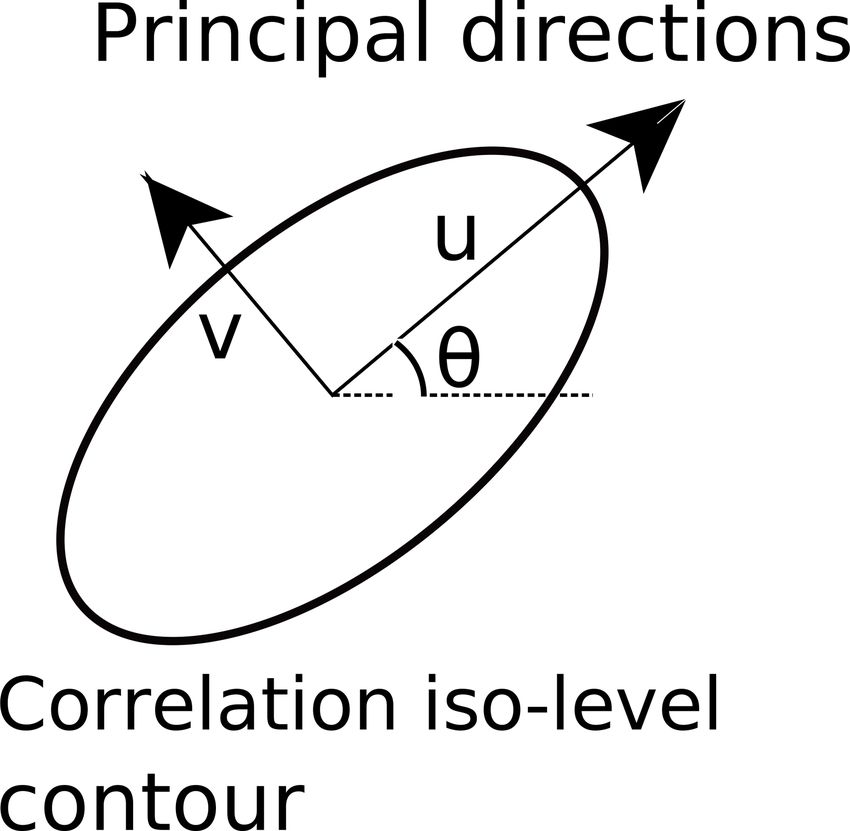
Figure 1. Representation of a generic ellipse that represents the geo-
in situ data so that land–sea boundary effects are properly
statistical geometric anisotropy of a wind or wave field. Supposing
captured for the subsequent coastal definition that will be u and v are the two principal directions of anisotropy, the anisotropy
based on the heterogeneity introduced by the presence of the ratio is R = uv > 1; symbol θ is the rotation angle of the field.
land boundary.
The geostatistical anisotropy in wind and wave fields
(Swail et al., 1999) can be a useful indicator of spatial struc- 2 Theoretical background
ture, affected by topo-bathymetric constraints that generate
substantial wave-driven gradients under strong met-ocean Given a spatio-temporal field X(s, t), where s stands for a 2-
conditions. In this text, the term “anisotropy” refers only D vector (zonal and meridional components) and t is time, it
to the geostatistical anisotropy, not the geophysical one. A is assumed that the iso-level contours of the correlation func-
wind or wave field that has a high anisotropy can present a tions are invariant, i.e. ellipses in two dimensions. The main
predominant wind or wave direction, respectively. It is well axes of these ellipses are termed u and v (see Fig. 1). The
known that the geostatistical anisotropy can be a measure to metric of the geometric anisotropy then becomes their ratio
define directional variation, e.g. for mineral configuration in R = uv (R ∈ [0, ∞); Chorti and Hristopulos, 2008; Petrakis
rocks (Amadei, 1996), for propagation velocity in heteroge- and Hristopulos, 2017). An R value close to unity means that
neous media (Crampin, 1984) or for seismic waves (Verdon u and v are isotropic, i.e. homogeneous across the different
et al., 2008). Similarly, topographically induced geostatisti- directional sectors. As R increases, the difference between
cal anisotropy affects coastal wind patterns that force wave the main axes increases, showing higher anisotropy at cer-
and current fields (Soomere, 2003). tain directional sectors.
The aim of this paper is to analyse the geostatistical Considering the ratio R as a 1-D random variable, it can
anisotropy of nearshore wind and waves for wave-driven be fitted to a probability distribution function. Such a fitting
coasts. From that, what follows is to propose a new quan- depends on theoretical and practical considerations. The pre-
titative and objective definition for the land–sea border that ferred shape is determined by looking at statistical character-
benefits from these high-resolution (spatial and temporal) istics such as mean, variance, skewness and kurtosis, or by
fields and from the underlying process-based knowledge. examining the similarity between quantiles (dataset versus
This definition can be useful to determine a set of criteria theoretical probability distribution) using a quantile–quantile
for numerical purposes (e.g. nesting coastal domains) but plot. The more direct candidates to fit variable R are (a) the
also for more practically oriented applications (e.g. offshore log-normal function, where the probability distribution of its
limit for outfall dispersion). The analysis is based on a set of log-transform is Gaussian (Aitchison and Brown, 1958), and
high-resolution wind and wave fields in the latter case us- (b) the log-logistic function, with a logistic probability distri-
ing a well-tested code such as SWAN (Simulating Waves bution for the log-transformed variable. A logistic distribu-
Nearshore; Booij et al., 1999; van der Westhuysen et al., tion has a probability density function of the following form:
2007; WISE Group, 2007; Zijlema, 2010). The numerical re- 1
sults, pertaining to a micro-tidal environment to avoid any f (x) = exp((x − m)/s)(1 + exp((x − m)/s))−2 , (1)
s
distortion of spatial patterns by tides, will be subject to com-
putationally inexpensive statistical methods to characterize where m is its location parameter and s is its scale parameter.
spatial structures. Following this approach, the paper is struc- Sklar’s theorem (Sklar, 1959) expresses the multivariate
tured as follows. Section 2 introduces the theoretical back- joint probability structure of two variables x and y as the
ground. Section 3 describes the study area, and the method- product of their cumulative probability distributions F (x)
ology is presented in Sect. 4. Section 5 lists the main results, and G(y), and a 2-D copula. The interval of variation
which are discussed in Sect. 6, followed by some conclusions in F (x), G(y) is [0, 1] and a 2-D Gaussian copula has the
in Sect. 7. following form:
Ocean Sci., 15, 113–126, 2019 www.ocean-sci.net/15/113/2019/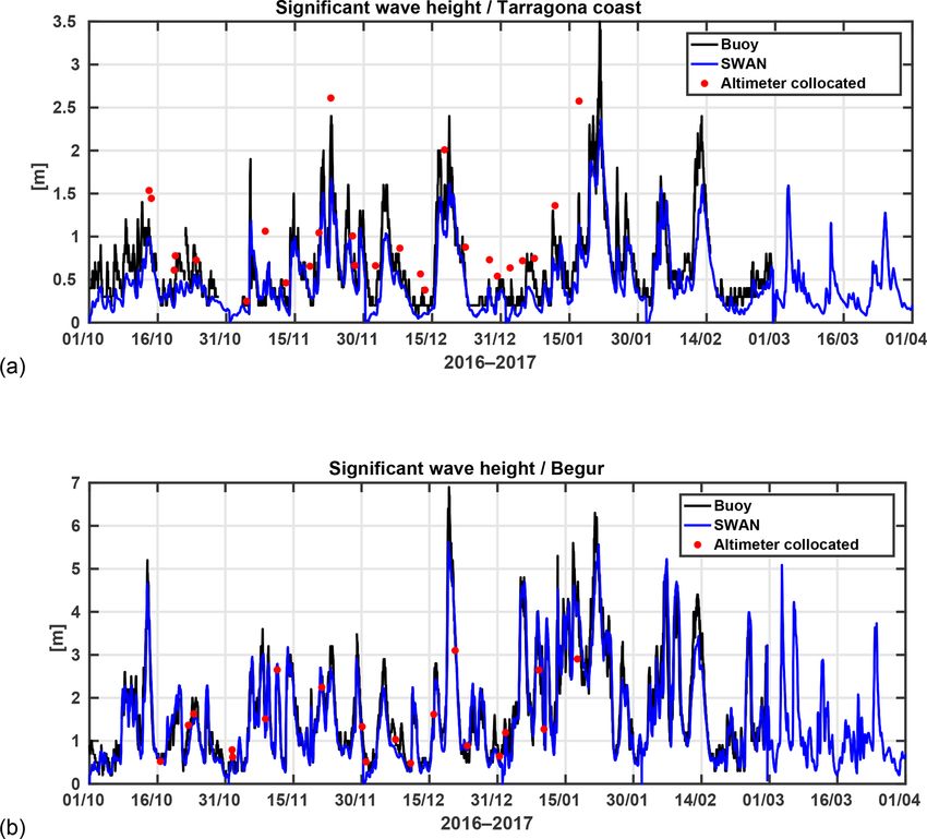
A. Sánchez-Arcilla et al.: The land–sea coastal border                                                                                         115

Figure 2. Study area showing the gradients in topo-bathymetry that exert a strong control over the resulting met-ocean conditions. The four
transects (red lines) used to estimate the limit of the coastal fringe are depicted, located in (from south to north) (a) Ebro Delta, (b) Tarragona,
(c) Badalona and (d) Begur. The map also shows the Puertos del Estado (PdE) buoys and the division of the Catalan coast into the northern,
central and southern sections (different colours on the land).

                                                                            orological driving, have not been considered in this initial
                         (F (x)) 8−1Z
                      8−1Z          (G(y))                                  analysis. The focus is on the Spanish north-eastern Mediter-
                                                    1
Cρ (F (x), G(y)) =                              q                           ranean coast, where we have in situ and altimeter support-
                                        2π 1 − ρ12  2                       ing data. Moreover, the continental shelf varies from 10 km
                         −∞         −∞
                         (                      )                           to more than 100 km in an alongshore distance of less than
                            s 2 − 2ρ12 st + t 2                             500 km. The wind fields are affected (most frequent wind
                      exp −             2
                                                 dsdt,            (2)
                                2 1 − ρ12                                   direction is from land, approximately corresponding to the
                                                                            north-west) by the presence of a mountain chain roughly par-
where the correlation parameter −1 < ρ12 < 1 is used as the                 allel to the coastline and featuring several openings corre-
dependence parameter and 8 is the univariate standard nor-                  sponding to river valleys. The geometrical anisotropy anal-
mal distribution function (Embrechts et al., 2001). ρ12 = 0                 ysis was performed at four transects, characteristic of their
means total independence between the variables, whereas                     common topo-bathymetric features. They correspond to the
|ρ12 | = 1 means total dependence. Whenever a joint proba-                  following locations (from south-west to north-east): Ebro
bility structure has the form of a Gaussian copula, this struc-             (40.7◦ N, 0.87◦ E), Tarragona (41.12◦ N, 1.25◦ E), Mataró
ture can be applied without excessive computational cost (Li                (41.53◦ N, 2.45◦ E) and Begur (42.28◦ N, 3.02◦ E) (Fig. 2).
et al., 2014; Rueda et al., 2016) compared, for instance, to                   The north-western Mediterranean presents a particularly
an Archimedean copula approach (Wahl et al., 2011; Lin-Ye                   intense wind forcing, which is shaped by local orography
et al., 2016; Okhrin et al., 2013).                                         (Jordi et al., 2011; Lebeaupin Brossier et al., 2012). The
                                                                            Pyrenees mountain chain across the strip of land connect-
3   Study area                                                              ing the Iberian Peninsula to the European continent forces
                                                                            a strong northern wind flux following the French–Spanish
The selected pilot site is the wave-driven and micro-tidal en-              Mediterranean coast (Nicolle et al., 2009; Schaeffer et al.,
vironment of the western Mediterranean Sea (Fig. 2), where                  2011; Obermann-Hellhund et al., 2017). This same wind pat-
enough validated met-ocean simulations exist and where the                  tern is channelled by the river valleys resulting in a north-
spatial wind/wave structure will not be distorted by tidal forc-            western orientation for winds blowing from land to sea fur-
ing. Current fields, slower to respond to the overlying mete-               ther down along the coast (Cerralbo et al., 2015) for latitudes

www.ocean-sci.net/15/113/2019/                                                                                 Ocean Sci., 15, 113–126, 2019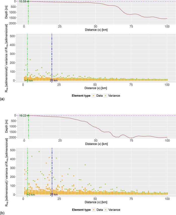
116                                                                  A. Sánchez-Arcilla et al.: The land–sea coastal border

southward of 41◦ N. The most frequently observed patterns
are thus from the north in the coastal sector closer to the
Pyrenees barrier and from the north-west further south, con-
ditioned by the river valleys and gaps in the coastal parallel
mountains (Obermann et al., 2016; Lin-Ye et al., 2016). The
second most frequent pattern corresponds to western winds,
associated with atmospheric depressions in northern Europe
(Barnston and Livezey, 1987; Trigo et al., 2002; Lin-Ye et al.,
2017). Easterly winds are frequent during the summer, trig-
gered by an intense high-pressure area over the British Isles.
   The most common wave fields in the northwestern
Mediterranean Sea correspond to the wind-sea spectral band
driven by easterly, northerly and north-westerly winds (Li-
onello and Sanna, 2005; Bolaños et al., 2009). Because of
the semi-enclosed character of the basin, the waves are fetch-
limited, with maximum trajectory lengths around 600 km,
one-sixth of the average distance that a wave train trav-
els across the Atlantic (García et al., 1993). The aver-          Figure 3. Flow chart summarizing the methodology used in this pa-
age wave climate in the north-western Mediterranean Sea           per. The dashed blue rectangle represents the input data, and the
presents a mean significant wave height (Hs ) of 0.78 m at        dashed red rectangle indicates the output data. The wind velocity
the southern part of the Catalan coast, near the Ebro Delta       is obtained from an external source, and it was validated in Martin
and slightly lower values (around 0.72 m) further north and       et al. (2006). The rest of the steps have been carried out for this anal-
close to the French border. The spatial distribution of wave      ysis. Rectangles indicate data generation (input/output), and rhom-
storms presents an opposite trend, with maximum Hs be-            buses indicate the subsequent analyses of the proposed methodol-
                                                                  ogy.
tween 5.48 m in the southern sector and 5.85 m at the north-
ern coastal stretch (Bolaños et al., 2009). Future projections
(Casas-Prat and Sierra, 2013) indicate, for the interval 2071–
2100 and the A1B scenario (IPCC, 2000), a variation in
the significant wave height around ±10%, whereas the same         there should be a geostatistical boundary to the value of this
variable for a 50-year return period exhibits rates of change     anisotropy that could help define a coastal boundary.
around ±20 %. Additionally, the variability in large-scale in-       The wind fields have been provided by the UK Met Office
dices (i.e. North Atlantic Oscillation, NAO; East Atlantic Os-    from their Unified Model (Cullen, 1993) for weather and cli-
cillation, EA; or Scandinavian Oscillation) may drive sig-        mate applications. This code solves the compressible, non-
nificant changes in wave-storm components (Lin-Ye et al.,         hydrostatic equations of motion with semi-Lagrangian ad-
2017).                                                            vection and semi-implicit time stepping, including suitable
                                                                  parameterizations for sub-grid scale processes such as con-
                                                                  vection, boundary layer turbulence, radiation, cloud micro-
                                                                  physics and orographic drag (Brown et al., 2012). There are
4     Methods                                                     two atmospheric prognostics: the dry one (three-dimensional
                                                                  wind components, potential temperature, Exner pressure and
The approach suggested for assessing the geostatistical           density) and the moist one (specific humidity and prognostic
anisotropy of wind and wave fields is schematized in Fig. 3.      cloud fields (Walters et al., 2011). Both long- and short-wave
It requires high-resolution met-ocean fields to determine how     radiation (from the Sun and the Earth itself) are included, and
the covariance of the geostatistical anisotropies of wind and     the effect of aerosols reflecting radiation is taken into con-
wave fields evolve with distance to the land–sea border. The      sideration. These wind data have been validated in previous
starting point is wind and associated wave fields, as the sug-    works, such as in Martin et al. (2006).
gested candidates for reflecting the heterogeneity induced           The computational domain of the wind field spans the
by coastal topo-bathymetry. Although other definitions of         whole Mediterranean Sea using a regular grid with spacing of
the coastal boundary can be based on river plumes or bio-         17 km and a time step of 1 h. The wave fields have been cal-
geochemical processes, it has been intended to focus on a         culated with the SWAN code, covering the same geograph-
more hydro-dynamical expression of such a boundary for            ical domain and with an equal time step of 1 h. SWAN is a
wave-driven coasts. It is intended to show that, as one ap-       spectral wave model based on the wave action balance equa-
proaches the coast, the wind and the wave fields should           tion (Booij et al., 1999; Zijlema, 2010) that includes non-
present a greater geostatistical anisotropy, i.e. they should     linear interactions at various depths and dissipation processes
display predominant wind and wave directions. Furthermore,        (i.e. whitecapping, bottom friction, wave breaking). It applies

Ocean Sci., 15, 113–126, 2019                                                                     www.ocean-sci.net/15/113/2019/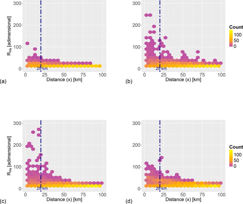
A. Sánchez-Arcilla et al.: The land–sea coastal border                                                                       117

a fully implicit numerical scheme for propagation in geo-            Heat maps are used to represent the spatial distribution of
graphical and spectral spaces that is unconditionally stable.     the geostatistical anisotropy, showing how the density of R
   SWAN employs an unstructured grid with spatial resolu-         behaves as a function of distance to the coast and time (see
tions of 600 m–40 km, denser near the land–sea boundary.          Figs. 6 and 7). These maps are scatter plots that act as a
Mesh sizes are proportional to bathymetry gradients and dis-      2-D histogram, in which two variables (in this case R and
tance to the coastline, following the same criteria than in       distance to the coast) are grouped in pre-defined intervals.
Pallarés et al. (2017). Such a non-structured-grid approach       The elements selected to aggregate samples for the heat map
avoids nesting and internal boundary conditions, while main-      are hexagons with 5 km side and a scale for anisotropy of
taining a good spatial resolution to capture bottom and coast-    20 units for both RVw and RHs . Both R and its variance are
line irregularity (submarine canyons and capes or pro-deltas      calculated on a discrete number of distances to the coast-
that are found in the Catalan continental shelf). Furthermore,    line, assuming that the width of the fringe affected by bound-
unstructured meshes are well suited to tackle non-linear ef-      ary effects is below 100 km for this coastal sector (Sánchez-
fects (Qi et al., 2009; Roland et al., 2012; Roland and Ard-      Arcilla and Simpson, 2002). From here, as is with signifi-
huin, 2014). The resulting wave fields have been validated        cant wave height to determine the presence of wave storms
with two directional wave buoys at the northern (Begur, de-       (Eastoe et al., 2013; Bernardara et al., 2014), the proposed
ployed at 1200 m) and southern (Tarragona coastal buoy, de-       coastal zone limit is the cutting point where the variance in R
ployed at 15 m) ends of the domain, managed by Puertos del        is equal to the 90th percentile of the total R variance span-
Estado (Fig. 2). Altimeter data from three satellites (CryoSat,   ning a fringe between 0 and 100 km:
Jason-2 and Jason-3) are also used as a complementary ob-
servational source. The simulation period ranges from Octo-       l = 90th percentile of var RHs (0 km ≤ x ≤ 100 km) . (4)
ber 2016 to March 2017.
                                                                  This cutting point has shown, as expected, larger stability for
   Once obtained the wave outputs, the empirical semi-
                                                                  the wave field than for the forcing wind patterns. The varia-
variograms for the significant wave height and the wind ve-
                                                                  tion in RHs with coastal distance x (Fig. 7) indicates for ref-
locity at 10 m are estimated. In order to have enough data, the
                                                                  erence the 20 km distance where satellite data offer enough
spatial radius of influence is assumed to be 5 km, plus time
                                                                  robustness (Cavaleri and Sclavo, 2006; Janssen et al., 2007;
blocks of 24 h. From these semi-variograms, the anisotropy
                                                                  Durrant et al., 2009). The plot also displays depth against x.
for the wave height (RHs ) and the wind velocity (RVw ) is es-
                                                                  The obtained RVw and RHs values were fitted to a probabil-
timated along the four transects in Fig. 2.
                                                                  ity distribution, empirically selecting the log-normal function
   Distance to the coast (x) and water depth (h) are selected
                                                                  for the inverse of RVw and the log-logistic function for RHs .
as independent variables for analysing the anisotropy spatial
                                                                  Once the marginal distributions are estimated, the depen-
patterns. RVw and RHs are taken to represent the behaviour of
                                                                  dence structure of the joint probability is adjusted to a Gaus-
met-ocean conditions under the effect of the land–sea bound-
                                                                  sian copula (see Sect. 2).
ary (in this initial analysis height/depth gradients in topo-
bathymetry). Hence, RVw and RHs have been interpolated
(1 km spacing) along a 100 km transect perpendicular to the       5   Results
coast (see Fig. 2), considering periods of 24 h, long enough
for the waves to respond to the acting wind forcing.              The modelled wave heights (Hs ) have been validated with
   The geostatistical anisotropy needs to be computed on a        buoys from the Puertos del Estado monitoring network and
regular grid and therefore both wind velocity (Vw ) and sig-      available altimeter data (Jason-2, CryoSat and Jason-3). Two
nificant wave height (Hs ) have been interpolated on a rect-      locations have been selected, located at the southern (Tarrag-
angular mesh, first on a grid of 1 km then to a finer mesh of     ona) and northern (Begur) coastal sectors (Figs. 4 and 5). The
10 m.                                                             Hs buoy data show good agreement with the simulated Hs ,
   The interpolation method used in this case is the inverse      quantified in Table 1 and in Figs. 4 and 5.
distance weighted (IDW) interpolation, which estimates the           In general, the wave model performs better for deep wa-
value at an interpolated location (x) as the weighted average     ters than for coastal waters. The standard deviation is higher
of neighbouring points with weights w(x) given by                 in the model than in the observations. At Begur, the bias and
            1                                                     the scatter index are lower, whereas the RMSE is higher (Ta-
w(x) =              .                                      (3)    ble 1). At the same buoy, the correlation coefficient is near
         d(x, xi )p
                                                                  95 % and the difference between standard deviations is lower
Here, xi is a neighbouring point, d is the Euclidean distance     (0.2 m vs. 0.4 m). Note that the northern part of the Catalan
and p is the inverse distance weighting power. The IDW            coast is more energetic than the southern one (see Fig. 5).
power chosen is 1 for RVw and 3 for RHs and h, based on           For instance, in Begur the storm peaks can reach about 7 m,
a sensitivity analysis for this area and consistent with the      whereas at Tarragona the highest recordings are 3.5 m.
physical relation between wind velocity and generated wave           The collocated altimeter data have a positive bias in the
height.                                                           coastal zone, and the opposite (i.e. negative bias) in deep

www.ocean-sci.net/15/113/2019/                                                                  Ocean Sci., 15, 113–126, 2019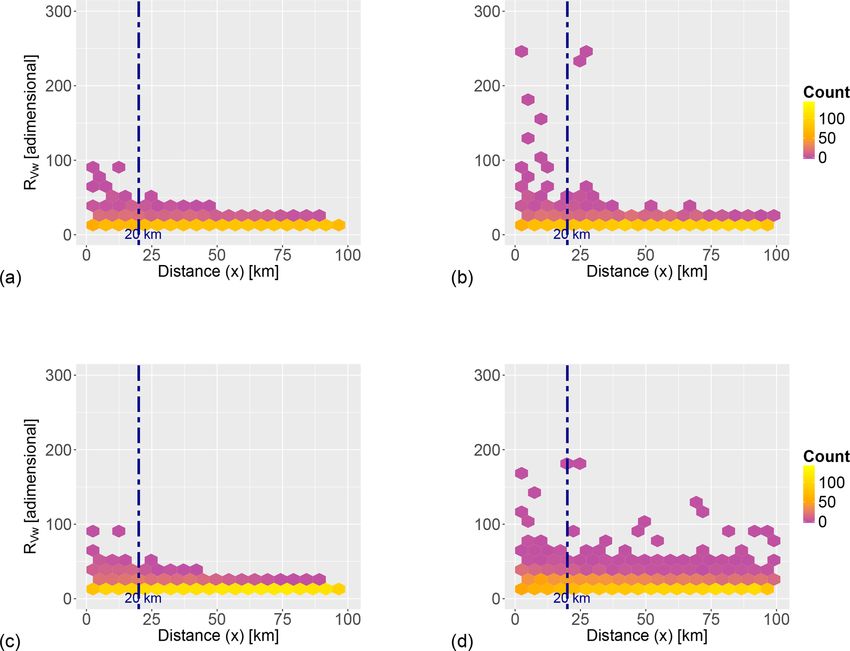
118 A. Sánchez-Arcilla et al.: The land–sea coastal border
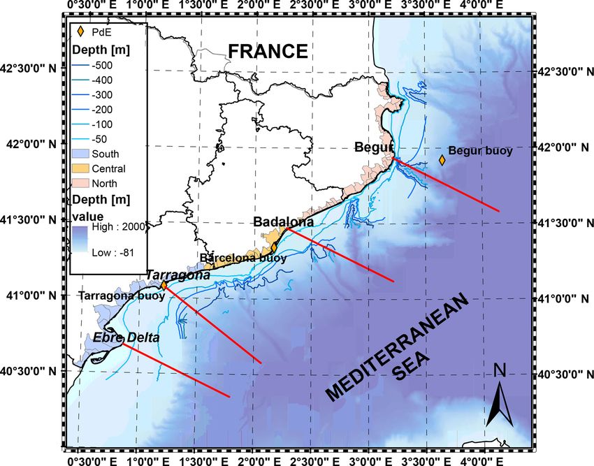
Table 1. Statistics of the agreement between numerical significant
wave height fields (SWAN model) and observations in terms of root
mean square error (RMSE), bias and scatter index (SI) for the con-
trol points at the southern and northern coastal sectors.
Buoy RMSE (m) Bias (m) SI (%)
Tarragona coastal buoy 0.248 −0.132 0.502
Begur 0.393 −0.087 0.249
turning point at about 40 km in all transects (Figs. 8 and 9)
and, thus, a higher level of consistency. From December to
January, there are some winds and waves registered within
20 km of the coast that present higher RVw and RHs ; how-
ever, they are so few that the variances in RVw and RHs in
this area do not differ from warmer seasons. Therefore, there
is not a clear seasonality to the RVw or the RHs . The coastal
zone limit l, corresponding to the 90th percentile of the total
variance (fringe between 0 and 100 km), is calculated from
Eq. (4) (Figs. 8 and 9) and is 3 km. It is consistent with the
time interval (month of study) and location (sector).
In order to find a copula structure, marginal probabil-
ity distributions for the two anisotropies are needed. Skew-
ness and kurtosis from the analysed data show that the in-
verse anisotropy of Vw follows a log-normal distribution,
while the anisotropy of Hs follows a log-logistic distribution.
Quantile–quantile plots were used to assess the fit of each
probability function (not shown here) to its target dataset,
verifying that the selected samples can be adjusted to the
corresponding probability distributions. The joint probabil-
ity structure of the two anisotropies does not present any
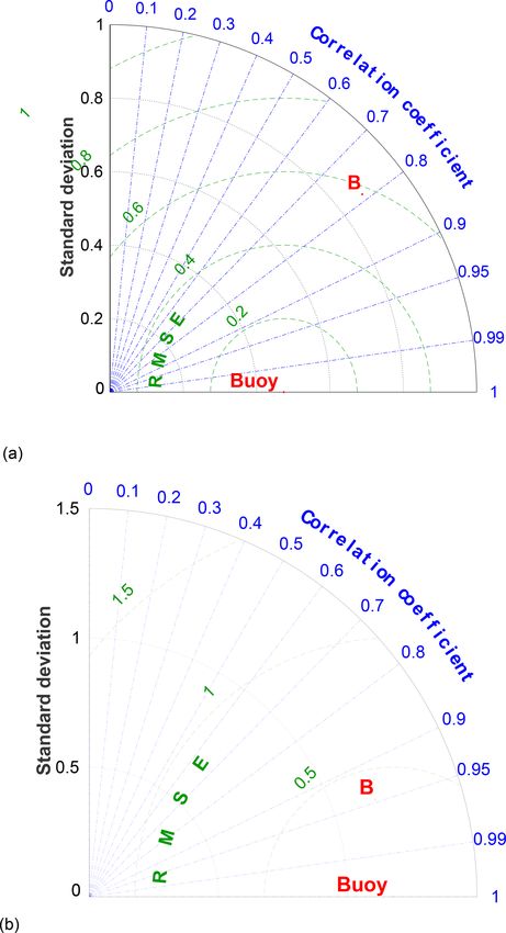
Figure 4. Taylor diagram for the significant wave height (Hs ) marked dependence for the upper-tail percentiles, suggesting
showing correlation, standard deviation and root mean square er- the use of a Gaussian copula, whose dependence parameter ρ
ror (RMSE) between numerical and observed data for (a) south sec- is shown in Fig. 10. The so obtained dependence ranges from
tor (Tarragona location) and (b) north sector (Begur location). The total independence (0) to a mild (|ρ12 | = 0.1) dependence be-
time period ranges from November 2016 to March 2017. tween RVw and RHs .
6 Discussion
waters. Nevertheless, there exists qualitative consistency be-
tween the in situ and remote-sensing sources. Additionally, The calculated anisotropies should be as robust as the start-
SWAN has been able to capture the regime switching and the ing wave or wind fields that are employed in the analysis. Be-
proper timing of the storms, despite that it tends to underes- cause of that, the SWAN code has been calibrated with local
timate the magnitude of the storm peaks. atmospheric and hydrodynamic conditions (Pallarés et al.,
RVw and RHs have been analysed with heat maps (Figs. 6 2017). Special emphasis has been put on using high-quality
and 7) and scatter plots (Figs. 8 and 9). RVw presents values wind fields, both for the direct assessment linked to meteo-
that span from 1 to 250 and display a dependence on coastal rological fields and for the indirect effect they exert on the
distance (Fig. 6), featuring a combination of anisotropy close behaviour of the forced hydrodynamics. The results show,
to the land boundary (0 to 20 km) and then a more isotropic as expected, a higher level of robustness for the wave-based
behaviour towards the offshore region (up to 100 km), al- geostatistical anisotropy, where the calculations used an un-
though with a rich variability. The wind fields present, in structured grid and a locally adjusted whitecapping term cal-
summary, a decreasing variance from 0 to 100 km with a ibration (Pallarés et al., 2014). The cell size has been deter-
pronounced slope from 0 to about 40 km (southern sector) mined as a function of depth and distance to the coast, con-
or even further offshore (northern sector) and then an almost sistently with the transect analyses performed in the paper.
asymptotical trend. RHs behaves similarly to RVw , but with a The application of an unstructured grid allows for reducing
Ocean Sci., 15, 113–126, 2019 www.ocean-sci.net/15/113/2019/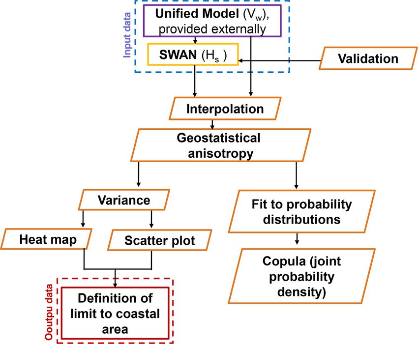
A. Sánchez-Arcilla et al.: The land–sea coastal border                                                                                 119

Figure 5. Comparison of numerically simulated significant wave height (SWAN model) with observations for (a) south sector (Tarragona
location) and (b) north sector (Begur location) for the period October 2016 to March 2017. The red dots are altimeter data (Jason-2, Jason-3
and CryoSat).

computational costs (by about 50 %) and the troublesome im-             where the boundary will be likely located. This suggests a
position of internal boundaries.                                        combined approach using numerical fields and satellite data
   This leads to an efficient determination of the coastal water        supplemented by along-track in situ observations, all suitably
boundary that contains some of its common geometric set-                interpolated in space and time to provide a picture that is as
tings (e.g. bathymetric gradients affecting wave fields). Other         consistent as possible.
processes, such as the continental discharge are of course not             The values of Vw , Hs and h obtained through the IDW in-
captured by the present analysis and would require a simi-              terpolation, using an IDW weighting from 1 to 3, are sim-
lar approach based on the resulting circulation fields, which           ilar and reasonable. For marine variables the weight of 3
would certainly capture the regions of fresh-water influence            has been selected to account for the influence of the clos-
and wave–current interactions (Staneva et al., 2016). How-              est neighbours based on the water inertia (which is 3 orders
ever, the performance of the wave model has shown com-                  of magnitude larger than for air). The proposed IDW power
monalities with previous studies. For instance, the good per-           for Vw is smaller because gas is more turbulent than water
formance of spectral models at the Begur buoy can be found              and thus should have a smaller spatial dependence. The ob-
in multi-model comparisons (see Bertotti et al., 2012), and             tained pattern for RVw is consistent for the four selected tran-
also the consistent underestimation under storm peaks (Cav-             sects in the study area, showing a mostly isotropic behaviour
aleri, 2009).                                                           for coastal distances from 0 to 100 km. Higher values of RVw
   The anisotropy-based approach will lead to different re-             at distances from the coast below 20 km (see Fig. 6) indi-
sults depending on met-ocean conditions (wave conditions in             cate a clear directional spread of winds within the coastal
our case), requiring a reliable simulation of both average and          fringe, linked to orographic control such as channelling by
extreme patterns, as shown by the validation process (e.g.              local mountains and river valleys.
see Figs. 4 and 5). The transfer of energy from the coastal                Despite the fact that the results are based on Novem-
to the offshore domain and vice versa may condition the re-             ber 2016 and February 2017, the spatial trends of the
sults of the analysis for areas near the transition, which is

www.ocean-sci.net/15/113/2019/                                                                           Ocean Sci., 15, 113–126, 2019
120                                                                            A. Sánchez-Arcilla et al.: The land–sea coastal border

Figure 6. Heat map of the geostatistical anisotropy ratio of the wind velocity (RVw ) against distance to the coast for (a) south control transect
(near the Ebro Delta), (b) central-south transect (near Tarragona harbour), (c) central-north transect (near Mataró harbour) and (d) north
control transect (near Begur cape). The elements selected to aggregate samples for the heat map are hexagons with 5 km side and a scale
for anisotropy of 20 units. The counts are the number of elements within a hexagon. A rough limit of the order of magnitude for the direct
applicability of remote-sensing data (20 km) is also shown (dashed blue line). All plots correspond to February 2017.

anisotropy were coherent throughout the simulation period,                 pronounced for transects with more stable atmospheric con-
thus exhibiting the robustness of the methodology.                         ditions. The link between RHs and land-originated winds
   The numerical wind fields present errors below 2 m s−1                  can be appreciated by the shift from a homogeneous to
(Martin et al., 2006), which means that the Vw calculated can              anisotropic behaviour in the northern- most transect (Begur)
well represent actual wind conditions. The RVw is lower in                 where the effect of Vw on Hs is only evident up to 38 km from
the Ebro Delta (Fig. 6a) than at Tarragona (Fig. 6b) due to                the coast. Note that the Ebro Delta shows a more isotropic
the fact that the orography at the Ebro Delta is flat, and wind            value at the coastal zone. This area presents a wider continen-
blows from a wide range of directions; whereas Tarragona                   tal shelf than the other profiles, where wave dissipation and
features mountain chains that channel the winds into a more                refraction tend to be more homogeneous. Henceforth, more
limited directional subset. The anisotropy pattern at Begur                anisotropic winds plus a steeper profile may be considered
(Fig. 6d) may be explained by the strong mistral and eastern               as the main reasons for the discrepancies among the beach
winds (Obermann et al., 2016; Obermann-Hellhund et al.,                    profiles.
2017) that both affect nearshore and deep waters.                             Such behaviour of RHs with coastal distance parallels
   Hence, the behaviour of RVw near the coast can show                     that of particulate matter diffusivity, which tends to become
sharp local variations due to the joint effect of orography,               isotropic at around 10 km (Romero et al., 2013) from the
mesoscale circulation and large-scale circulation, all affect-             land–water boundary. The degree of geostatistical anisotropy
ing wind strength and directionality. However, the seasonal-               in diffusivity is physically related to eddy kinetic energy,
ity does not affect RVw as much. In all cases, Vw becomes                  which varies as x 5/4 (x being separation distance) for depths
more isotropic towards the offshore, denoting a decreasing                 below 20 m (Gràcia et al., 1999). A steep bottom slope will
control by the land–water boundary.                                        favour deep-water wave behaviour at relatively short dis-
   The RHs pattern is similar, with wave fields show-                      tances from the coast, as shown by the distinctive behaviour
ing boundary effects (mainly in directional properties) for                of RHs for coasts of different slope. However, although
coastal distances below 50 km, which has also been consid-                 RHs presents greater variance (more outliers) for steep slopes
ered an order of magnitude estimate for land wind effects.                 (e.g. due to the combination of deep- and shallow-water wave
Farther from the coast there is a clear trend to isotropy, more            regimes as in the central-north transect near Mataró harbour),

Ocean Sci., 15, 113–126, 2019                                                                              www.ocean-sci.net/15/113/2019/
A. Sánchez-Arcilla et al.: The land–sea coastal border                                                                                    121

Figure 7. Heat map of the geostatistical anisotropy ratio of significant wave height (RHs ) against distance to the coast for (a) south control
transect (near the Ebro Delta), (b) central-south transect (near Tarragona harbour), (c) central-north transect (near Mataró harbour) and
(d) north control transect (near Begur cape). The elements selected to aggregate samples for the heat map are hexagons with 5 km side and
a scale for anisotropy of 20 units. The counts are the number of elements within a hexagon. A rough limit of the order of magnitude for the
direct applicability of remote-sensing data (20 km) is also shown (dashed blue line). All plots correspond to February 2017.

the gradient of RHs with distance to the coast is similar for all         transects (see Fig. 10). There seems to be a strong wind chan-
types of bathymetry considered, suggesting a generic value                nelling aligned with the main river valleys (Sánchez-Arcilla
of the proposed approach. This is also true for any time of               et al., 2014; Rafols et al., 2017) in February and March, dom-
the year.                                                                 inating the local wave fields. The ρ parameter should reflect
   The coastal boundaries suggested by Sánchez-Arcilla and                this spatial and temporal variation, resulting in a coastal zone
Simpson (2002) for the Catalan Coast can be 0.1–0.6 km                    width that will be a function of the prevailing met-ocean
(frictional coupling of fluids between shelf and nearshore),              drivers and should thus be considered a dynamic concept.
10 km (non-linear coupling between shelf and slope) and                      The resulting coastal definition can be data (numerical
1 km (non-linear coupling between shelf and nearshore),                   or observed) driven, being directly applicable to any region
among other suggested values of the same order of magni-                  with a forecasting system or with enough coverage of in situ
tude. The l provided in our analysis is slightly larger than              plus satellite data. The proposed criteria appear to work well
the value given for the frictional coupling of fluids between             for wave-dominated and micro-tidal environments; and al-
shelf and nearshore, whereas it is similar or smaller than in             though suitable for any combination of factors, their appli-
the non-linear couplings. Nevertheless, the orders of magni-              cation to macro-tidal regimes or river-discharge-dominated
tude are similar.                                                         areas should account for the corresponding signature in the
   The ρ parameter of the Gaussian copula, characterizing                 hydrodynamic fields. Under these conditions, the preferred
the dependence structure among RVw and RHs , reflects a                   variable could change to current velocity or to temperature,
certain similarity to the spatial behaviour for both variables            considering in all cases the effect of spatial resolution in the
(see Figs. 6 and 7). The overall mutual dependence of RVw                 results.
and RHs is strongest for the northern-most transect (Begur),
where the topo-bathymetric control of the Pyrenees and their
submerged signature becomes better defined. Such mutual
dependence gets weaker for the central and southern coastal

www.ocean-sci.net/15/113/2019/                                                                             Ocean Sci., 15, 113–126, 2019
122 A. Sánchez-Arcilla et al.: The land–sea coastal border
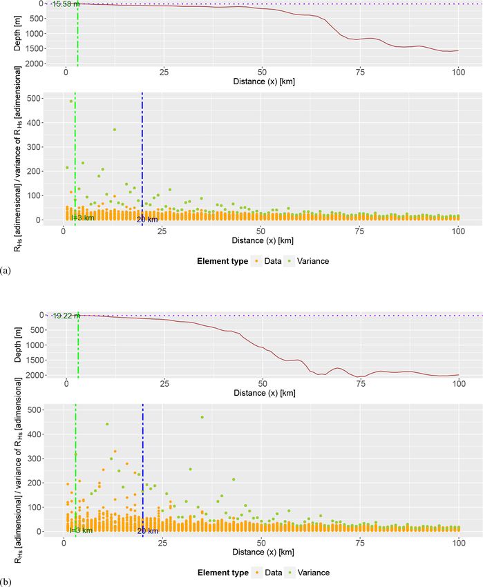
Figure 8. Relation for winter conditions (February 2017) between distance to the coast x, depth and anisotropy ratio of significant wave
height (RHs ) from shore to 100 km offshore. Locations are (a) south control transect (near the Ebro Delta) and (b) central-north transect
(near Mataró harbour). The distance of 20 km, which has been suggested as an approximate order of magnitude limit for direct applicability
of remote-sensing data, is also shown (dashed blue line) together with the variance in RHs across the transect. From here, the coastal zone
anisotropy-based boundary has been calculated and is also depicted. A dash-dotted green line delimits its horizontal distance from the coast,
whereas a dotted purple line denotes its elevation.
7 Conclusions variable that reflects such an influence (here it has been il-
lustrated with wind velocity and significant wave height) and
The proposed coastal fringe (water sub-domain) definition can be easily automated for any field, numerical or observa-
is based on an objective estimation of the geostatistical tional, that presents enough resolution.
anisotropy as a proxy for the influence of the land border. The methodology has been tested with numerically gen-
The suggested statistical assessment can be applied to any erated fields and validated with datasets from Puertos del
Ocean Sci., 15, 113–126, 2019 www.ocean-sci.net/15/113/2019/A. Sánchez-Arcilla et al.: The land–sea coastal border 123 Figure 9. Relation for autumn conditions (November 2016) between distance to the coast x, depth (a) and geostatistical anisotropy ratio of significant wave height (RHs ) from shore to 100 km offshore. Locations are (a) south control transect (near the Ebro Delta) and (b) central- north transect (near Mataró harbour). The distance of 20 km, which has been suggested as a rough order of magnitude limit for direct applicability of remote-sensing data, is also shown (dashed blue line) together with the variance in RHs across the transect. From here, the coastal zone anisotropy-based boundary has been calculated and is also depicted. A dash-dotted green line delimits its horizontal distance from the coast, whereas a dotted purple line denotes its elevation. Estado buoys and altimeter. Anisotropies of wind velocity by the land–sea border, demonstrating the topo-bathymetric and significant wave height have been extracted along a set control on met-ocean factors. This control depends on topo- of characteristic profiles spanning widths of up to 100 km graphic (mountain chains and river valleys) and bathymetric (see Fig. 2), considered sufficient for the relatively narrow (bottom slope, submarine canyons or pro-deltas) features but shelves in the Spanish Mediterranean coast. The performed also on the energetic level of the prevailing weather, lead- analysis has shown how wind and wave fields are influenced ing to a dynamic definition of the coastal water domain. www.ocean-sci.net/15/113/2019/ Ocean Sci., 15, 113–126, 2019
124                                                                        A. Sánchez-Arcilla et al.: The land–sea coastal border

                                                                        Acknowledgements. This paper has been supported by the Eu-
                                                                        ropean project CEASELESS (H2020-730030-CEASELESS) and
                                                                        the Spanish national projects COBALTO (CTM2017-88036-R)
                                                                        and ECOSISTEMA-BC (CTM2017-84275-R). As a group, we
                                                                        would like to thank the Secretary of Universities and Research
                                                                        of the department of economics of the Government of Catalonia
                                                                        (ref. 2014SGR1253). We duly thank the Meteorological Office
                                                                        of the UK for the provided wind fields, Copernicus Marine
                                                                        Environment Monitoring Service for the altimeter data and the
                                                                        public body Puertos del Estado for the in situ measurements.

                                                                        Edited by: Joanna Staneva
                                                                        Reviewed by: three anonymous referees

Figure 10. Copula parameters ρ of the proposed Gaussian copu-
las for all considered profiles: (a) south control transect (near the   References
Ebro Delta), (b) central-south transect (near Tarragona harbour),
(c) central-north transect (near Mataró harbour) and (d) north con-     Aitchison, J. and Brown, J. A. C.: The lognormal distribution with
trol transect (near Begur cape). The plot shows the variation with        special reference to its uses in economics, J. Polit. Econ., 66,
time (horizontal axis) between November 2016 and March 2017.              370–371, 1958.
The parameters are placed in a manner such that they start from         Amadei, B.: Importance of anisotropy when estimating and mea-
January.                                                                  suring in situ stresses in rock, in: International Journal of Rock
                                                                          Mechanics and Mining Sciences & Geomechanics Abstracts,
                                                                          vol. 33, Elsevier, Pergamon, 293–325, 1996.
The resulting widths, based on variance variation, span dis-            Barbier, E. B., Hacker, S. D., Kennedy, C., Koch, E. W.,
tances in the kilometre range, depending on bottom slope                  Stier, A. C., and Silliman, B. R.: The value of estuarine
and coastal plan-shape geometry. The correlation between                  and coastal ecosystem services, Ecol. Monogr., 81, 169–193,
                                                                          https://doi.org/10.1890/10-1510.1, 2011.
the wind- and wave-based definitions (i.e. the mutual de-
                                                                        Barnston, A. G. and Livezey, R. E.: Classification, Seasonality and
pendence among RVw and RHs ) seems to be stronger in
                                                                          Persistence of Low-Frequency Atmospheric Circulation Patterns,
the northern-most parts of the study area, where the topo-                Mon. Weather Rev., 115, 1083–1126, 1987.
bathymetric control is most prominent.                                  Bernardara, P., Mazas, F., Kergadallan, X., and Hamm, L.: A
   This new definition of the coastal zone can be useful for              two-step framework for over-threshold modelling of environ-
setting up standards to delimit this transitional fringe, facil-          mental extremes, Nat. Hazards Earth Syst. Sci., 14, 635–647,
itating the selection of processes and boundary conditions                https://doi.org/10.5194/nhess-14-635-2014, 2014.
for modelling and providing an objective coastal zone limit             Bertotti, L., Bidlot, J., Bunney, C., Cavaleri, L., Passeri, L. D.,
for impact assessments. Such an approach can also support                 Gomez, M., Lefèvre, J., Paccagnella, T., Torrisi, L., Valentini,
directional and asymmetric measures of error and the under-               A., and Vocino, A.: Performance of different forecast systems
lying metrics (between model and data), leading to improved               in an exceptional storm in the Western Mediterranean Sea, Q. J.
                                                                          Roy. Meteorol. Soc., 138, 34–55, https://doi.org/10.1002/qj.892,
products and standards in the coastal zone.
                                                                          2012.
                                                                        Bolaños, R., Jorda, G., Cateura, J., Lopez, J., Puigdefabregas, J.,
                                                                          Gomez, J., and Espino, M.: The XIOM: 20 years of a regional
Data availability. Model outputs are available upon request to the        coastal observatory in the Spanish Catalan coast, J. Mar. Syst.,
first author.                                                             77, 237–260, 2009.
                                                                        Booij, N., Ris, R., and Holthuijsen, L.: A third-generation wave
                                                                          model for coastal regions, Part I, Model description and valida-
Author contributions. ASA led the research and the writing pro-           tion, J. Geophys. Res., 104, 7649–7666, 1999.
cess. All authors contributed equally to this work.                     Brown, A., Milton, S., Cullen, M., Golding, B., Mitchell, J., and
                                                                          Shelly, A.: Unified modeling and prediction of weather and cli-
                                                                          mate: A 25-year journey, B. Am. Meteorol. Soc., 93, 1865–1877,
Competing interests. The authors declare that they have no conflict       2012.
of interest.                                                            Bulleri, F. and Chapman, M. G.: The introduction of coastal
                                                                          infrastructure as a driver of change in marine environ-
                                                                          ments, J. Appl. Ecol., 47, 26–35, https://doi.org/10.1111/j.1365-
Special issue statement. This article is part of the special issue        2664.2009.01751.x, 2010.
“Coastal modelling and uncertainties based on CMEMS products”.          Casas-Prat, M. and Sierra, J.: Projected Future Wave Climate in the
It is not associated with a conference.                                   NW Mediterranean Sea, J. Geophys. Res.-Oceans, 118, 3548–
                                                                          3568, 2013.

Ocean Sci., 15, 113–126, 2019                                                                         www.ocean-sci.net/15/113/2019/
A. Sánchez-Arcilla et al.: The land–sea coastal border 125
Cavaleri, L.: Wave modeling – missing the peaks, J. Phys. Wave Height Data, J. Atmos. Ocean. Tech., 24, 1665–1677,
Oceanogr., 39, 2757–2778, 2009. https://doi.org/10.1175/JTECH2069.1, 2007.
Cavaleri, L. and Sclavo, M.: The calibration of wind and wave Jordi, A., Basterretxea, G., and Wang, D.-P.: Local versus remote
model data in the Mediterranean Sea, Coast. Eng., 53, 613–627, wind effects on the coastal circulation of a microtidal bay in the
2006. Mediterranean Sea, J. Mar. Syst., 88, 312–322, 2011.
Cavaleri, L., Bertotti, L., and Pezzutto, P.: Accuracy of al- Lebeaupin Brossier, C., Béranger, K., and Drobinski, P.: Ocean re-
timeter data in inner and coastal seas, Ocean Sci. Discuss., sponse to strong precipitation events in the Gulf of Lions (north-
https://doi.org/10.5194/os-2018-81, in review, 2018. western Mediterranean Sea): A sensitivity study, Ocean Dynam.,
Cerralbo, P., Grifoll, M., Moré, J., Bravo, M., Sairouní Afif, 62, 213–226, 2012.
A., and Espino, M.: Wind variability in a coastal area (Al- Li, F., van Gelder, P., Vrijling, J., Callaghan, D., Jongejan, R., and
facs Bay, Ebro River delta), Adv. Sci. Res., 12, 11–21, Ranasinghe, R.: Probabilistic estimation of coastal dune erosion
https://doi.org/10.5194/asr-12-11-2015, 2015. and recession by statistical simulation of storm events, Appl.
Chorti, A. and Hristopulos, D. T.: Nonparametric identification Ocean Res., 47, 53–62, 2014.
of anisotropic (elliptic) correlations in spatially distributed data Lin-Ye, J., García-León, M., Gràcia, V., and Sánchez-Arcilla, A.:
sets, IEEE T. Signal Proc., 56, 4738–4751, 2008. A multivariate statistical model of extreme events: An ap-
Crampin, S.: An introduction to wave propagation in anisotropic plication to the Catalan coast, Coast. Eng., 117, 138–156,
media, Geophys. J. Int., 76, 17–28, 1984. https://doi.org/10.1016/j.coastaleng.2016.08.002, 2016.
Cullen, M. J. P.: The unified forecast/climate model, Meteorol. Lin-Ye, J., García-León, M., Gràcia, V., Ortego, M. I., Lionello, P.,
Mag., 122, 81–94, 1993. and Sánchez-Arcilla, A.: Multivariate statistical modelling of fu-
Durrant, T. H., Greenslade, D. J. M., and Simmonds, I.: ture marine storms, Appl. Ocean Res., 65, 192–205, 2017.
Validation of Jason-1 and Envisat Remotely Sensed Lionello, P. and Sanna, A.: Mediterranean wave climate variability
Wave Heights, J. Atmos. Ocean. Tech., 26, 123–134, and its links with NAO and Indian Monsoon, Clim. Dynam., 25,
https://doi.org/10.1175/2008JTECHO598.1, 2009. 611–623, https://doi.org/10.1007/s00382-005-0025-4, 2005.
Eastoe, E., Koukoulas, S., and Jonathan, P.: Statistical measures of Martin, G. M., Ringer, M. A., Pope, V. D., Jones, A., Dear-
extremal dependence illustrated using measured sea surface ele- den, C., and Hinton, T. J.: The physical properties of the at-
vations from a neighbourhood of coastal locations, Ocean Eng., mosphere in the new Hadley Centre Global Environmental
62, 68–77, 2013. Model (HadGEM1). Part I: Model description and global clima-
Embrechts, P., Lindskog, F., and McNeil, A.: Modelling depen- tology, J. Climate, 19, 1274–1301, 2006.
dence with copulas, Rapport technique, Département de math- Miller, S. T. K., Keim, B. D., Talbot, R. W., and Mao, H.: Sea
ématiques, Institut Fédéral de Technologie de Zurich, Zurich, breeze: Structure, forecasting, and impacts, Rev. Geophys., 41,
2001. 1011, https://doi.org/10.1029/2003RG000124, 2003.
Estournel, C., Durrieu de Madron, X., Marsaleix, P., Auclair, Nicolle, A., Garreau, P., and Liorzou, B.: Modelling for anchovy
F., Julliand, C., and Vehil, R.: Observation and modeling of recruitment studies in the Gulf of Lions (Western Mediterranean
the winter coastal oceanic circulation in the Gulf of Lion un- Sea), Ocean Dynam., 59, 953–968, 2009.
der wind conditions influenced by the continental orography Obermann, A., Bastin, S., Belamari, S., Conte, D., Gaertner, M. A.,
(FETCH experiment), J. Geophys. Res.-Oceans, 108, 8059, Li, L., and Ahrens, B.: Mistral and Tramontane wind speed and
https://doi.org/10.1029/2001JC000825, 2003. wind direction patterns in regional climate simulations, Clim.
García, M., Sánchez-Arcilla, A., Sierra, J., Sospedra, J., and Gómez, Dynam., 51, 1059–1076, 2016.
J.: Wind waves off the Ebro Delta, NM Mediterranean, Mar. Obermann-Hellhund, A., Conte, D., Somot, S., Torma, C. Z., and
Syst., 4, 235–262, 1993. Ahrens, B.: Mistral and Tramontane wind systems in climate
Geleynse, N., Voller, V. R., Paola, C., and Ganti, V.: Characteriza- simulations from 1950 to 2100, Clim. Dynam., 50, 693–703,
tion of river delta shorelines, Geophys. Res. Lett., 39, L17402, 2017.
https://doi.org/10.1029/2012GL052845, 2012. Okhrin, O., Okhrin, Y., and Schmid, W.: Properties of hierarchical
Gràcia, V., Jimenez, J. A., Sánchez-Arcilla, A., Guillén, J., and Archimedean copulas, Statist. Risk Model. Appl. Finance Insur.,
Palanques, A.: Short-term relatively deep sedimentation on the 30, 21–54, 2013.
Ebro delta coast. Opening the closure depth, in: 26th Interna- Pallarés, E., Sánchez-Arcilla, A., and Espino, M.: Wave energy
tional Conference on Coastal Engineering, 22–26 June 1998, balance in wave models (SWAN) for semi-enclosed domains–
Copenhaguen, Denmark, 2902–2912, 1999. appication to the Catalan coast, Cont. Shelf Res., 87, 41–53,
Halpern, B. S., Walbridge, S., Selkoe, K. A., Kappel, C. V., Micheli, 2014.
F., D’agrosa, C., Bruno, J. F., Casey, K. S., Ebert, C., Fox, H. E., Pallarés, E., López, J., Espino, M., and Sánchez-Arcilla, A.: Com-
and Fujita, R.: A global map of human impact on marine ecosys- parison between nested grids and unstructured grids for a high-
tems, Science, 319, 948–952, 2008. resolution wave forecasting system in the western Mediterranean
IPCC: Summary for policymakers. Emissions Scenarios, in: A Spe- sea, J. Operat. Oceanogr., 10, 45–58, 2017.
cial Report of Working Group III of the Intergovernmental Panel Petrakis, M. P. and Hristopulos, D. T.: Non-parametric approxima-
of Climate Change, Tech. rep., IPCC, Cambridge University tions for anisotropy estimation in two-dimensional differentiable
Press, Cambridge, 2000. Gaussian random fields, Stoch. Environ. Res. Risk A., 31, 1853–
Janssen, P. A. E. M., Abdalla, S., Hersbach, H., and Bid- 1870, 2017.
lot, J.-R.: Error Estimation of Buoy, Satellite, and Model Qi, J., Chen, C., Beardsley, R. C., Perrie, W., Cowles, G.
W., and Lai, Z.: An unstructured-grid finite-volume sur-
www.ocean-sci.net/15/113/2019/ Ocean Sci., 15, 113–126, 2019126 A. Sánchez-Arcilla et al.: The land–sea coastal border
face wave model (FVCOM-SWAVE): Implementation, val- Sklar, A.: Fonctions dé repartition à n dimension et leurs marges,
idations and applications, Ocean Model., 28, 153–166, Université Paris 8, Paris, France, 1959.
https://doi.org/10.1016/j.ocemod.2009.01.007, 2009. Soomere, T.: Anisotropy of wind and wave regimes in the Baltic
Rafols, L., Grifoll, M., Jorda, G., Espino, M., Sairouni, A., Proper, J. Sea Res., 49, 305–316, 2003.
and Bravo, M.: Shelf Circulation Induced by an Oro- Staneva, J., Wahle, K., Günther, H., and Stanev, E.: Coupling of
graphic Wind Jet, J. Geophys. Res.-Oceans, 122, 8225–8245, wave and circulation models in coastal-ocean predicting systems:
https://doi.org/10.1002/2017JC012773, 2017. a case study for the German Bight, Ocean Sci., 12, 797–806,
Roland, A. and Ardhuin, F.: On the developments of spectral wave https://doi.org/10.5194/os-12-797-2016, 2016.
models: Numerics and parameterizations for the coastal ocean, Swail, V., Komen, G., Ryabinin, V., Holt, M., Taylor, P. K., and Bid-
Ocean Dynam., 64, 833–846, 2014. lot, J.: Wind waves in the Global Ocean Observing System, in:
Roland, A., Zhang, Y. J., Wang, H. V., Meng, Y., Teng, Y.-C., OCEANOBS99, Proc. of the Int. Conf. on the Ocean Observing
Maderich, V., Brovchenko, I., Dutour-Sikiric, M., and Zanke, System for Climate, St. Raphael, France, 1999.
U.: A fully coupled 3D wave-current interaction model on Trigo, I. F., Bigg, G. R., and Davies, T. D.: Climatology of cyclo-
unstructured grids, J. Geophys. Res.-Oceans, 117, C00J33, genesis mechanisms in the Mediterranean, Mon. Weather Rev.,
https://doi.org/10.1029/2012JC007952, 2012. 130, 549–569, 2002.
Romero, L., Uchiyama, Y., Ohlmann, J. C., McWilliams, J. C., and van der Westhuysen, A., Zijlema, M., and Battjes, J.: Nonlinear
Siegel, D. A.: Simulations of nearshore particle-pair dispersion in saturation-based whitecapping dissipation in SWAN for deep and
Southern California, J. Phys. Oceanogr., 43, 1862–1879, 2013. shallow water, Coast. Eng., 54, 151–170, 2007.
Rueda, A., Camus, P., Tomás, A., Vitousek, S., and Méndez, F.: Verdon, J. P., Angus, D. A., Kendall, J. M., and Hall, S. A.: The ef-
A multivariate extreme wave and storm surge climate emula- fect of microstructure and nonlinear stress on anisotropic seismic
tor based on weather patterns, Ocean Model., 104, 242–251, velocities, Geophysics, 73, D41–D51, 2008.
https://doi.org/10.1016/j.ocemod.2016.06.008, 2016. Wahl, T., Jensen, J., and Mudersbach, C.: A multivariate statistical
Sánchez-Arcilla, A. and Simpson, J. H.: The narrow shelf con- model for advanced storm surge analyses in the North Sea, Coast.
cept: couplings and fluxes, Cont. Shelf Res., 22, 153–172, Eng. Proc., 1, 19, 2011.
https://doi.org/10.1016/S0278-4343(01)00052-8, 2002. Walters, D. N., Best, M. J., Bushell, A. C., Copsey, D., Edwards,
Sánchez-Arcilla, A., García, M., and Gràcia, V.: Hydro- J. M., Falloon, P. D., Harris, C. M., Lock, A. P., Manners, J.
morphodynamic modelling in Mediterranean storms – errors C., Morcrette, C. J., Roberts, M. J., Stratton, R. A., Webster, S.,
and uncertainties under sharp gradients, Nat. Hazards Earth Wilkinson, J. M., Willett, M. R., Boutle, I. A., Earnshaw, P. D.,
Syst. Sci., 14, 2993–3004, https://doi.org/10.5194/nhess-14- Hill, P. G., MacLachlan, C., Martin, G. M., Moufouma-Okia, W.,
2993-2014, 2014. Palmer, M. D., Petch, J. C., Rooney, G. G., Scaife, A. A., and
Sánchez-Arcilla, A., García-León, M., Gràcia, V., Devoy, R., Stan- Williams, K. D.: The Met Office Unified Model Global Atmo-
ica, A., and Gault, J.: Managing coastal environments under cli- sphere 3.0/3.1 and JULES Global Land 3.0/3.1 configurations,
mate change: pathways to adaptation, Sci. Total Environ., 572, Geosci. Model Dev., 4, 919–941, https://doi.org/10.5194/gmd-4-
1336–1352, 2016. 919-2011, 2011.
Schaeffer, A., Molcard, A., Forget, P., Fraunié, P., and Garreau, P.: Wiese, A., Staneva, J., Schulz-Stellenfleth, J., Behrens, A.,
Generation mechanisms for mesoscale eddies in the Gulf of Li- Fenoglio-Marc, L., and Bidlot, J.-R.: Synergy of wind wave
ons: Radar observation and modeling, Ocean Dynam., 61, 1587– model simulations and satellite observations during extreme
1609, 2011. events, Ocean Sci., 14, 1503–1521, https://doi.org/10.5194/os-
Shaw, J. B., Wolinsky, M. A., Paola, C., and Voller, V. 14-1503-2018, 2018.
R.: An image-based method for shoreline mapping WISE Group: Wave modelling-the state of the art, Prog. Oceanogr.,
on complex coasts, Geophys. Res. Lett., 35, L12405, 75, 603–674, 2007.
https://doi.org/10.1029/2008GL033963, 2008. Zijlema, M.: Computation of wind-wave spectra in coastal waters
with {SWAN} on unstructured grids, Coast. Eng., 57, 267–277,
https://doi.org/10.1016/j.coastaleng.2009.10.011, 2010.
Ocean Sci., 15, 113–126, 2019 www.ocean-sci.net/15/113/2019/You can also read