KIEL WORKING PAPER Covid-19 Shocking Global Value Chains* - Kiel Institute for the ...
←
→
Page content transcription
If your browser does not render page correctly, please read the page content below

KIEL
WORKING
PAPER
Covid-19 Shocking
Global Value Chains*

                                                           No. 2167 September 2020
Peter Eppinger, Gabriel Felbermayr, Oliver Krebs and Bohdan Kukharsky

Kiel Institute for the World Economy
ISSN 1862–1155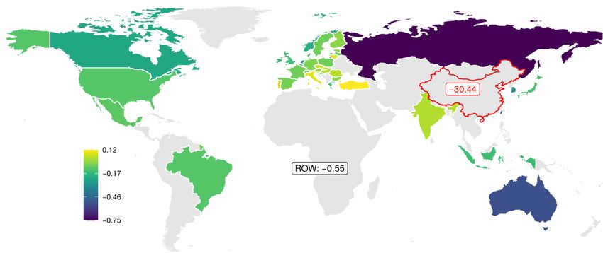
KIEL WORKING PAPER                         NO. 2167 | SEPTEMBER 2020

    ABSTRACT
    COVID-19 SHOCKING GLOBAL VALUE
    CHAINS*
    Peter Eppinger, Gabriel Felbermayr, Oliver Krebs and Bohdan Kukharsky
    In early 2020, the disease Covid-19 caused a drastic lockdown of the Chinese economy. We
    use a quantitative trade model with input-output linkages to gauge the effects of this adverse
    supply shock in China on the global economy through international trade and global value
    chains (GVCs). We find moderate welfare losses in most countries outside of China, while
    a few countries even gain from the shock due to trade diversion. As a key methodological
    contribution, we quantify the role of GVCs (in contrast to final goods trade) in transmitting
    the shock. In a hypothetical world without GVCs, the welfare loss due to the Covid-19 shock
    in China is reduced by 40% in the median country. In several other countries, the effects are
    magnified or reversed for several countries. Had the U.S. unilaterally repatriated GVCs, the
    country would have incurred a substantial welfare loss while its exposure to the shock would
    have barely changed.

    Keywords: Covid-19, quantitative trade model, input-output linkages, global value chains,
    supply chain contagion, shock transmission
    JEL classification: F11, F12, F14, F17, F62

    Peter Eppinger                             Gabriel Felbermayr                          Oliver Krebs
    University of Tübingen                     Kiel Institute for the World Economy        University of Tübingen

    Bohdan Kukharskyy
    City University of New York

    *We thank Wilhelm Kohler for valuable comments. Jaqueline Hansen provided excellent research assistance. All remaining
    errors are our own.

    The responsibility for the contents of this publication rests with the author, not the Institute. Since working papers are of a
    preliminary nature, it may be useful to contact the author of a particular issue about results or caveats before referring to,
    or quoting, a paper. Any comments should be sent directly to the author.
1      I NTRODUCTION
The disease Covid-19, caused by a novel coronavirus (SARS-CoV-2), was first diagnosed in De-
cember 2019 in China’s Hubei province. Within weeks the outbreak turned into an epidemic, and
by mid-February 2020 most Chinese provinces were under complete or partial lockdown. Even
before the virus infected millions of people worldwide, this major shock to Chinese production
and consumption affected the global economy through ‘supply chain contagion’ (Baldwin and
Tomiura, 2020, and Gerschel et al., 2020). As early as February 2020, firms around the world
began experiencing disruptions of their production processes due to a lack of intermediate inputs
from China.1 Soon thereafter, newspapers around the world were filled with speculations on the
global economic repercussions of the Covid-19 shock in China (see, e.g., Reuters, 2020, and The
Guardian, 2020). These events have fueled a public discourse about the reliance on Chinese inputs,
with politicians on both sides of the Atlantic calling for a ‘decoupling’ or ‘repatriation’ of global
value chains (GVCs), in particular those involving China (Irwin, 2020, and Baldwin and Evenett,
2020).
    This paper informs the ongoing debate by providing the following three contributions. First,
we present a model-based quantification of the global repercussions of Covid-19 via international
trade and GVCs. Given the importance of China as a pivotal hub in GVCs, we focus on the well-
defined initial Covid-19 shock in China in January–February 2020, i.e., before the disease turned
into a pandemic.2 Second, and most importantly, we quantify the relevance of GVCs in the shock
transmission by reconsidering the same Covid-19 shock in China occurring in a counterfactual
world in which intermediate goods trade via GVCs has been shut down. Notably, our counterfac-
tual world still permits international trade in final goods and the existence of sectoral linkages in
domestic value chains. Third, and related, we study the repercussions of the shock after the U.S.
has unilaterally decoupled from global (or Chinese) value chains, as recently discussed in policy
circles.
    The framework we use for our analysis is a generalization of the quantitative Ricardian trade
model with multiple sectors and input-output (I-O) linkages. Three key features of the model
make it particularly suited for our purpose: First, it includes both domestic and international I-O
linkages (as in Caliendo and Parro, 2015), and hence describes how sectors are affected directly
and indirectly through GVCs. Second, it distinguishes trade costs for intermediate inputs and final
goods (as in Antràs and Chor, 2018), which allows us to isolate the role of GVCs. Third, we allow
    1
      Between February 1 and March 5, 2020, the majority of the global top 5000 multinational enterprises (MNEs)
revised their earnings forecasts for fiscal year 2020 and more than two thirds of the top 100 MNEs issued statements
on the impact of Covid-19 on their business (UNCTAD, 2020). See also individual reports on Apple Inc. and Airbus
SE in New York Times (2020) and The Economist (2020).
    2
      Until the end of February, Covid-19 infections were still predominantly confined to China (see Dong et al., 2020,
and the discussion in Section 3.2).

                                                          1
for imperfect intersectoral mobility of labor (similar to Galle et al., 2018).
    We use the model and Chinese administrative data to back out the sectoral labor supply shocks
caused by Covid-19. To achieve this, we estimate the initial output drop in Chinese sectors from
monthly time series. Related to the methodology in Allen et al. (2020), this initial output drop
is conceptualized as the ‘zeroth degree’ effect of the shock in China, i.e., before any response by
the rest of the world. By inverting the model for the 0th degree effect, we recover the underlying
shocks to efficient labor supply by sector from the output drop. We calibrate the model based on
the World Input-Output Database (WIOD, Timmer et al., 2015) to study the global repercussions
of the Covid-19 shock in China in a range of counterfactual scenarios. These scenarios are best
thought of as answering the question of how the world economy would have responded if Covid-19
had permanently reduced production in China but had not spread internationally.3
    Our three main findings are as follows: First, our baseline scenario predicts the effects of the
Covid-19 shock in China on welfare and real sectoral output for 43 countries (and the rest of
the world) in 2014, the most recent year covered in the WIOD. We find that, in the new general
equilibrium, China experiences a welfare loss of roughly -30%. At the same time, our model
predicts moderate spillovers of this shock to all other countries, with welfare effects ranging from
-0.75% in Russia to +0.12% in Turkey. Interestingly, nine (mostly European) countries experience
a moderate welfare gain from the shock due to trade diversion.
    Second, we isolate the role of GVCs in transmitting the shock. To this end, we shut down
GVCs by setting the cost of international trade in intermediate goods to infinity. Importantly, our
approach differs from the shutting down of all I-O linkages (as simulated in the seminal paper by
Caliendo and Parro, 2015) in allowing for domestic input trade. It also differs from a (gradual)
return to autarky (as simulated in the contemporaneous studies by Bonadio et al., 2020, and Sforza
and Steininger, 2020) in allowing for final goods trade. This counterfactual analysis corresponds to
a full repatriation of input provision of the type that is currently being discussed in some countries.
We then compare the shock transmission in this ‘no-GVCs’ scenario to our baseline predictions.
We find that shutting down GVCs reduces the welfare loss due to the Covid-19 shock in China by
40% for the median country, with pronounced heterogeneity across countries. Interestingly, in the
world without GVCs, the welfare losses are magnified for several countries, including Germany,
while they are reversed for other countries. Further analyses reveal that these results are mainly
driven by a decoupling from China and less from reduced GVC trade among all other countries.
The cross-country patterns are similar when GVCs are shut down only partially (rather than en-
tirely).
   3
     Notably, the main goal of these exercises is not to explain the actual global developments during the Covid-19
crisis in 2020, but to shed light on the global transmission of a major supply shock in China in a world economy that
is less integrated via GVCs.

                                                         2
Finally, we consider two policy scenarios of the U.S. repatriating value chains (i) from all other
countries or (ii) only from China, and then revisit the international transmission of the Covid-19
shock in China after the policy change. We find that fully repatriating U.S. value chains causes a
welfare loss of around 1.56% in the U.S. but hardly reduces U.S. exposure to the shock in China.
Furthermore, even if the U.S. could anticipate that the next adverse shock were to come from
China, and even if it could fully eliminate any imports of inputs from China, the U.S. welfare
loss due to the Covid-19 shock in China would be reduced merely from -0.11% to -0.08%. The
reduction in shock exposure must be evaluated against the direct welfare cost to the U.S. from
repatriating value chains from China, which amounts to -0.12%. We obtain similar qualitative
conclusions when considering less extreme scenarios of increasing trade barriers by 10% or 100%.
These analyses inform the ongoing debate, in the U.S. but also in the European Union and other
economies, about the costs and benefits of repatriating value chains. Our findings suggest that,
even in the face of large and long-lasting shocks abroad, repatriating value chains can hardly be an
optimal policy from an economic welfare perspective.
The Covid-19 pandemic has given rise to a fast growing literature studying the economic impact
of the disease and policy responses. The macroeconomic effects of the pandemic have been as-
sessed in several important contributions, including Baqaee and Farhi (2020a,b), Eichenbaum et al.
(2020), Fornaro and Wolf (2020), Guerrieri et al. (2020), and McKibbin and Fernando (2020). Our
paper is most closely related to the contemporaneous papers by Bonadio et al. (2020) and Sforza
and Steininger (2020), who consider GVCs in the context of Covid-19. These papers aim at quan-
tifying the impact of quarantine and social distancing measures taken in many countries around the
world, while we focus on the initial shock in China. Moreover, in our analysis, we can distinctly
pin down the contribution of GVCs (as opposed to trade in general) to the transmission of the
Covid-19 shock. Barrot et al. (2020), Bodenstein et al. (2020), and Inoue and Todo (2020) (among
others) study the role of domestic supply chains in a closed economy setup.
More broadly, our paper relates to the theoretical and empirical literature on the role of pro-
duction networks in shaping economic outcomes (see Carvalho and Tahbaz-Salehi, 2019, for a
recent overview). The propagation of shocks through supply chains has been studied extensively
both theoretically (see, e.g., Acemoglu et al., 2012, and Acemoglu and Tahbaz-Salehi, 2020) and
empirically in the context of natural disasters (see, e.g., Barrot and Sauvagnat, 2016, and Carvalho
et al., 2016, and Boehm et al., 2019). We complement these studies with a quantitative exercise
demonstrating that, for some countries, the Covid-19 shock in China might have been exacerbated
(rather than mitigated) in the absence of GVCs.
The paper is organized as follows. We present the model in Section 2. Section 3 describes the
data and empirical methodology. Section 4 presents and discusses the simulation results. Finally,
we draw some conclusions in Section 5.
32 T HE MODEL
Our baseline model is strongly related to Antràs and Chor (2018), who extend the multi-sector
Eaton-Kortum model by Caliendo and Parro (2015) to allow for varying trade costs for intermedi-
ates and final goods, thus being able to exactly match each entry in multi-country I-O tables (i.e.,
each flow by country-sector and country-use category). A new element that we introduce into this
framework is heterogeneity of workers in terms of the efficient labor they can provide to different
sectors. This approach has two important advantages for our application. First, it adds realism by
acknowledging the imperfect mobility of labor across sectors that seems appropriate in our setting.
Second, it allows us to analyze the reductions in efficient labor supply by sector that are at the heart
of the Covid-19 shock.
2.1 E NDOWMENTS
We consider a world economy consisting of J countries indexed by j and i, in which S sectors
indexed by s and r can be active. Each country is endowed with an aggregate mass of worker-
consumers Lj , with each individual inelastically supplying one unit of raw labor. Workers are
immobile across countries and we consider different scenarios concerning their mobility across
sectors, ranging from immobility in the short run over imperfect mobility in the medium run and
perfect mobility in the long run. In the latter two cases the number of workers Ljs in each country-
sector is endogenous in equilibrium, while it is exogenous in the case of immobility.
2.2 P REFERENCES AND SECTOR CHOICE
P REFERENCES . All consumers in country j draw utility from the consumption of a Cobb-Douglas
compound good, which itself consists of CES compound goods from each of the sectors s ∈
{1, ..., S}. Aggregate consumption Cj in country j is given by
S
Y S
X
α
Cj = Cjs js , where αjs = 1, (1)
s=1 s=1
and αjs denotes expenditure shares on sectoral compound goods Cjs . Each Cjs is a CES aggregate
over a continuum of individual varieties ω ∈ [0, 1] produced within each sector:
Z 1 σsσ−1
s
σs −1
Cjs = xjs (ω) σs dω , (2)
0
where xjs (ω) is total final consumption in country j of variety ω from sector s, and σs > 1 is the
elasticity of substitution across varieties.
4S ECTORAL MOBILITY. We assume that if individual Ω in country j decides to work in sector s,
the efficient labor in this country-sector increases by δjs (Ω). Intuitively, these values ‘translating’
raw into efficient labor reflect both the applicability of a worker’s skills and training to a particular
sector and switching costs to this sector. The efficiency of labor δjs (Ω) is drawn by each individual
from sector- and country-specific Fréchet distributions with means δjs > 0 and shape parameter
ϕ > 1, such that the cumulative density function becomes
ϕ
δ
js
− 1 ϕ
δ −ϕ
Pr [δjs (Ω) ≤ δ] = e (
Γ 1− ϕ ) ,
where Γ (·) denotes the gamma function. The normalization of the scale parameter ensures that the
mean of δjs (Ω) for sector s across all workers in country j is exactly equal to δjs and independent
of our choice of ϕ. The parameter δjs will turn out to be our key shock parameter. A reduction in δjs
reduces the supply of efficient labor in the economy, as all workers draw on average lower values
δjs (Ω) for country-sector js. This drop captures the essence of the Covid-19 shock in China, as
workers are held back from going to work or operate under time-consuming or efficiency-reducing
constraints, such as additional hygiene measures or the requirement to work from home.
As explained above, we consider several scenarios with regard to worker mobility across sec-
tors. Under sectoral mobility, workers pick sector s if it offers them the highest compensation.
Therefore, given all compensations per unit of efficient labor wjs in all sectors s in country j we
can derive the number of workers Ljs who pick sector s as their workplace as
ϕ ϕ
δjs wjs
Ljs = Lj PS ϕ ϕ
. (3)
r=1 δjr wjr
Notice that our approach implies that wages per efficiency unit do not need to equalize across
sectors in equilibrium. More specifically, a sector increasing its wages will, on average, attract
workers that provide less efficient labor to this sector than those already working there.
Using the properties of the Fréchet distribution it is easy to show that the average wage wj paid
to each worker, i.e., the ex-ante expected wage, is the same in each sector in country j and given
by
S
! ϕ1
X ϕ ϕ
wj = δjs wjs . (4)
s=1
2.3 P RODUCTION
P RODUCTION . On the production side we assume that, in each country j, each sector s poten-
tially produces a continuum of varieties ω ∈ [0, 1] under perfect competition and with constant
5returns to scale. As in Caliendo and Parro (2015), production uses labor and CES compound
goods from potentially all sectors as intermediate goods.
More specifically, producers of variety ω in country j and sector s combine efficient labor units
ljs (ω) and intermediate goods mjrs (ω) from all sectors r ∈ {1, ..., S} in a Cobb-Douglas fashion:
S
!
Y
qjs (ω) = zjs (ω) ljs (ω)γjs mjrs (ω)γjrs , (5)
r=1
where γjs , γjrs ∈ [0, 1] are the cost shares of labor and intermediates from each sector in produc-
P
tion, and where γjs + Sr=1 γjrs = 1. Following Eaton and Kortum (2002), exogenous productiv-
ities zjs (ω) are drawn from country- and sector-specific Fréchet distributions with the cumulative
−εs
distribution functions Pr[zjs (ω) ≤ z] = e−Tjs z , where Tjs determines the average productivities
in each country j and sector s, and εs measures their dispersion across countries, which we assume
to satisfy εs > σs − 1. The compound intermediate goods mjrs (ω) are produced from individual
varieties ω using the same CES aggregator as specified in equation (2).
P RICES . Production technologies of all varieties within sector s and country j differ only with
respect to productivities. Perfect competition, therefore, implies that all producers in sector s and
country j face the same marginal production costs per efficiency unit cjs and set mill prices of
c
pjs (ω) = zjsjs(ω) .
All varieties can be traded subject to iceberg trade costs between any two countries i and
j. Following Antràs and Chor (2018), we assume that these trade costs depend not only on the
country pair ij and sector r of the traded good, but also on the use category u ∈ {1, . . . , S + 1},
which can be one of the S sectors using the variety as an intermediate or it can be final demand.
Thus, τijru ≥ 1 units have to be shipped from country i and sector r for one unit to arrive in
country j and use category u. The resulting price at which variety ω from sector r in country i is
offered to use category u in country j can be expressed as
cir τijru
pijru (ω) ≡ pir (ω) τijru = . (6)
zir (ω)
As prices depend on productivities, they inherit their stochastic nature. In particular, under the
assumption that variety ω from sector s is homogeneous across all possible producing countries,
firms and consumers buy them from the cheapest source, implying a price of min {pijru ; i ∈ J}.
Using the properties of the Fréchet distribution and following Eaton and Kortum (2002), we can
derive both the price Pjru of sector r compound goods paid in country j and use category u as well
6as the share πijru that country i makes up in use category u’s expenditure in country j on sector r:4
1−σ
1
" J #−1/εr
εr + 1 − σ r r X
Pjru = Γ Tir (cir τijru )−εr (7)
εr i=1
and
Tir [τijru cir ]−εr
πijru = PJ . (8)
k=1 Tkr [τkjru ckr ]−εr
C OSTS . Firms’ profit maximization and the Cobb-Douglas production structure imply that the
total expenditure Ejrs by sector s in country j on intermediates from sector r and its expenditure
on labor are given by
Ejrs = γjrs Rjs and Ljs wj = γjs Rjs , (9)
where Rjs denotes the total revenue of sector s in country j. Moreover, using the price indices (7),
the input bundle cost per efficient unit of output becomes
S
Y
γ γ
cjs = χjs wjsjs Pjrsjrs , (10)
r=1
−γjs QS −γ
with χjs = γjs r=1 γrjsrjs being a country- and sector-specific constant.
2.4 E QUILIBRIUM
E XPENDITURE AND CONSUMPTION . Balanced trade together with factor demands from equa-
tion (9), implies that aggregate expenditure Ejr(S+1) by consumers in any country j on goods from
sector r can be expressed as:
S
!
X
Ejr(S+1) = αjr γjs Rjs . (11)
s=1
Subsequently, aggregate consumer welfare or real expenditure can be derived by combining
expenditures (11) with the price indices (7) to obtain
PS
Ejr(S+1)
Cj = QSr=1 jrα . (12)
r=1 Pjr(S+1)
4
A detailed derivation of the price index and these shares can be found in Appendix A.1.
7G OODS MARKET CLEARING . In equilibrium, goods market clearing requires that the value of
production in country j and sector s equals the value of world final and intermediate goods demand
for that sector:
XJ XS+1
Ris = πijsu Ejsu . (13)
j=1 u=1
FACTOR M ARKET C LEARING . In equilibrium, wages adjust such that factor markets clear.
Specifically, combining sectoral labor compensation (9) with the definition of the per capita wage
given in (4) and the supply of sectoral labor (3) allows us to solve explicitly for the country- and
sector-specific wages per efficiency unit of labor as
1
P ϕ−1
S ϕ
(γjs Rjs ) ϕ
s=1 γjs Rjs
wjs = . (14)
δjs Lj
It is instructive to point out two extreme cases. First, as ϕ approaches infinity, all workers draw
the same parameter δjs for sector s in country j, and hence labor becomes perfectly mobile across
sectors. In this scenario, which is the standard case in the literature, the sectoral wage per efficiency
unit of labor simplifies to wj /δjs . Second, we will also consider a scenario of worker immobility,
in particular when modeling the immediate impact of the Covid-19 shock. In this case, equation
(3) no longer holds and Ljs is given exogenously instead. Also, sectoral per-capita wages no longer
equalize but can be obtained directly from sectoral factor market clearing as γjs Rjs /Ljs .5
E QUILIBRIUM CONDITIONS . An equilibrium in the model is defined by values of Pjru and Rjs
for all countries, sectors and use categories that satisfy the following equilibrium conditions given
all preference parameters αjs and σs , cost shares γjs and γjrs , sectoral and labor productivity
distribution parameters Tjs , δjs , εs and ϕ, and worker endowments Lj . The first set of equilibrium
conditions is obtained from the price index equations (7) after replacing marginal costs using (10)
and subsequently factor prices using (14). The second set of equilibrium conditions is obtained
from goods market clearing (13) after plugging in expenditures from (11) and (9) as well as trade
shares (8) combined with marginal costs (10) and factor prices (14).
E QUILIBRIUM IN CHANGES . Instead of solving the model in levels, we rely on the popular ‘exact
hat algebra’ by Dekle et al. (2007) to solve for counterfactual equilibria in response to a shock in
terms of changes. Denoting variables after the shock with a prime and their relative changes with
a hat we can restate the equilibrium as follows.
5
This scenario cannot be captured by letting ϕ approach 0 since, due to the nature of the Fréchet distribution, the
average productivity of workers is not well defined for ϕ ≤ 1.
8Given a shock defined by relative changes in average worker productivity draws δ̂ir , average
productivities T̂ir , trade costs τ̂ijru for all countries i, j, sectors r and use categories u, the equi-
librium of the model in changes consists of values P̂iru and R̂ir for all countries i, sectors r and
use categories u that satisfy the following equilibrium conditions given all αir , cost shares γir and
γirs , distributional parameters εr and ϕ, as well as labor endowments Li , trade shares πijru , and
revenues Rir in the ex-ante equilibrium:
" J
#−1/εr
X
P̂jru = πijru T̂ir (ĉir τ̂ijru )−εr , (15)
i=1
J S+1
1 XX ′
R̂ir = π̂ijru πijru Ejru , (16)
Rir j=1 u=1
where we use expenditures from (11) and (9), trade shares (8), marginal costs (10) and factor prices
(14), all expressed in changes:
S
!
X
′
Ejr(S+1) = αjr γjs R̂js Rjs , (17)
s=1
′
Ejru = γjru R̂ju Rju ∀u ≤ S , (18)
T̂ir (ĉir τ̂ijru )−εr
π̂ijru = PJ , (19)
k=1 πkjru T̂kr (ĉkr τ̂kjru )−εr
S
Y
γ γ
ĉjs = ŵjsjs P̂jrsjrs , (20)
r=1
ϕ1 PS ϕ−1
s=1 γjs R̂js Rjs
ϕ
R̂js P S
s=1 γjs Rjs
ŵjs = . (21)
δ̂js
3 DATA AND EMPIRICAL METHODOLOGY
In this section we first outline how the model is mapped to global data on trade in intermediate and
final goods from multi-country I-O tables. We then describe our estimation of the initial impact of
Covid-19 on the output of Chinese sectors using administrative data. Finally, we explain how we
9use the model to back out the sectoral labor supply shocks from the estimated output drop.
3.1 M APPING THE MODEL TO THE DATA
Our main data source is the most recent release of the WIOD, which provides annual time-series of
the world input-ouput tables from 2000 to 2014. It covers 43 countries, jointly accounting for more
than 85% of world GDP, and an artificial ‘rest of the world’ (see Table A.1 in the Appendix for a
list of countries). The input-output data are available at the level of 56 sectors classified according
to the International Standard Industrial Classification revision 4 (see Table A.2 in the Appendix for
a list of sectors). In our baseline analysis, we use the data from 2014, the latest available year.
We process the original data by applying the following three adjustments. First, we account
for the static nature of our model and follow Costinot and Rodriguez-Clare (2014) in recalculating
all flows in the WIOD as if positive inventory changes had been consumed and negative inven-
tory changes produced in the current period. Second, to ensure existence of the equilibrium in
a counterfactual world without GVCs, we need to ensure that fixed (exogenous) intermediate re-
quirements of different sectors can be met by an equivalent domestic supply when international
intermediate trade is shut down. To address this issue, we assume that each sector in each country
sources at least 1 USD worth of inputs domestically in all sectors from which it uses any inputs
in the data (similar to Antràs and Chor, 2018).6 Third, to make the WIOD consistent with our
theoretical framework, we purge it from aggregate trade imbalances (following the methodology
by Dekle et al. (2008) and Costinot and Rodriguez-Clare (2014)) and examine all shocks starting
from this counterfactual scenario.
From the WIOD we take initial values for the trade shares (πijru ) and the Cobb-Douglas struc-
ture of our model allows us to recover from the same data the values for cost shares (γir and γirs )
and expenditure shares (αjs ).7
We take the values for trade elasticities (εr ) from Felbermayr et al. (2018), who estimate them
from a structural gravity model. The sectoral elasticities are reported in column 2 of Table A.3.
We set the baseline sectoral labor mobility parameter (ϕ) to 3 and vary its value in the sensitivity
analysis.
3.2 E STIMATING THE INITIAL IMPACT OF C OVID -19 IN C HINESE SECTORS
To estimate the initial output drop in Chinese sectors due to Covid-19, we adopt an event-study
approach that is widely used in economics and finance (see MacKinlay, 1997). We exploit sectoral
6
It should be noted that this treatment of zeros does not significantly affect our baseline results, as the welfare
effects in all countries are identical to those reported below to at least 6 digits precision.
7
Notice that WIOD is the only data base that allows disentangling trade shares according to use category, thereby
allowing for use category specific trade costs τijru .
10time series from the National Bureau of Statistics (NBS) of China over three years before the
Covid-19 shock (the ‘estimation window’) to predict the counterfactual output in the absence of
the shock in January and February 2020 (the ‘event window’). The difference between observed
and predicted output in the event window is our estimate of the initial Covid-19 impact by sector.
Our choice of the event window in January–February 2020 exploits the exact timing of the
Covid-19 crisis. The first official, public mentioning of the disease dates from December 31, 2019
(when the cases were few), so the earliest economic impact can be expected in January 2020. Most
containment measures in China were then implemented over the course of the subsequent two
months. Notably, the spread of the virus was almost exclusively confined to China until late Febru-
ary. More specifically, data from Dong et al. (2020) show that on February 29, 92% of all globally
confirmed Covid-19 cases were recorded in China, with only 6,655 cases confirmed outside of
China (mostly concentrated in South Korea, Italy, and Iran). One week earlier, on February 22,
China’s share was at 98%, with only 1,578 infections confirmed outside of China (of which 634
were recorded on he cruise ship ‘Diamond Princess’). Not before March 11 did the WHO de-
clare Covid-19 a pandemic. While certain containment measures in China remained effective into
March and beyond, the disease had by then spread internationally. Hence, we cannot exclude the
possibility that the output data in these later months reflect also a response to international infec-
tions or to international repercussions of the initial shock in China. It is the latter channel that we
investigate in detail in our main analysis, but we want to rule it out in our estimate of the initial
shock. Thus, we do not consider data after February 2020 in this exercise.
We use monthly sector-level data on output (or more broadly, performance) from the NBS
of China. The NBS reports only cumulative numbers for the first two months of each year (not
for January and February separately), due to the Chinese spring festival. Hence, we construct
bi-monthly time series by sector. For the industrial sector (which encompasses mining, manufac-
turing, and utilities), we use data on operating revenues of industrial enterprises, deflated by the
sectoral producer price index (PPI). These data are reported for 41 sectors, which can be mapped
directly into 23 WIOD sectors, accounting for 57% of total Chinese output in the 2014 WIOD. For
the tertiary sector, we use different time series measuring performance (mostly revenues, appro-
priately deflated) in specific services, corresponding to 17 WIOD sectors (including retail trade,
telecommunications, and transport). We complement these data with the aggregate index of service
production in sectors for which more disaggregate data are unavailable (corresponding to 14% of
total Chinese output). Since monthly data for the Chinese primary sector are unavailable, we use
data from the industry ‘processing of food from agricultural products’ for this sector. Table A.2 in
the Appendix provides the details on the selected time series and a concordance table of NBS and
WIOD sectors (both following the International Standard Industrial Classification Rev. 4).
We denote the output of sector s in 2-month period t by Yst and define the annual (6-period)
11difference in output as ∆Yst ≡ Yst − Ys(t−6) . Our goal is to estimate the impact of the Covid-19
shock as the difference between the observed and expected output change in the first period of
2020 (i.e., the so-called ‘abnormal return’ in the event study literature):
Covid-19 impactst = ∆Yst − E[∆Yst ]. (22)
[
Our preferred estimator ∆Y st for the expected output change E[∆Yst ] is the seasonally differenced
model with a first-order autoregressive AR(1) disturbance:
∆Yst = ust , with ust = ρus(t−1) + est , (23)
where ust is the AR(1) disturbance, ρ is the autocorrelation parameter, and est is the i.i.d., mean-
zero, and normally distributed error term. This estimator is chosen to purge the bi-monthly time
series of sector-specific seasonality while taking into account the serial correlation present in the
data.8 Notably, equation (23) is estimated from bi-monthly time series over the pre-shock years
2017 to 2019, as is customary to ensure that the estimates are unaffected by the event itself, and it
dit for the first period of 2020.
is then used to predict ∆Y
Figure A.1 summarizes the estimates. It shows for each sector: the differenced time series, the
prediction of the differenced AR(1) model, and the predicted abnormal return in the first period of
2020 – our estimate of the initial impact of Covid-19.9 The estimates show that the impact was
dramatic. The average sectoral output declined by 30% compared to its expected value. The most
affected sector (textiles) experienced a drop of almost 60%, while output in land transport and
several other manufacturing sectors dropped by around 50% due to the virus and the lockdown.
Only few sectors experienced no significant drop or even a slight increase in output, in particular
the oil extraction and telecommunication services sectors. The latter example points the relevance
of I-O linkages for the estimated output drop, highlighting the need for backing out the underlying
sectoral labor supply shocks from the estimated output drop, which is what we do in the next
subsection.
The estimated effects are mapped to WIOD sectors according to Table A.2 and aggregated at
the level of WIOD sectors, weighted by initial values in January–February 2019. Table A.3 reports
in column 2 the estimated drop in output caused by Covid-19 for each WIOD sector in China.
8
The size of the estimated impact by sector hardly changes at all if we include a constant term in equation (23)
to allow for a trend in the growth rate. This model, as well as alternative models of the ARIMA class (adding, e.g.,
moving averages, or autoregressive disturbances of higher order) turn out to be inferior to the AR(1) model in most
sectors by the Akaike and Bayesian information criteria.
9
The autocorrelation plots for the AR(1) model residuals, depicted in Figure A.2, demonstrate that there is no
significant autocorrelation pattern remaining.
123.3 BACKING OUT LABOR SUPPLY SHOCKS
The estimated output drop in Chinese sectors due to Covid-19 reflects not only the underlying labor
supply shock in a given sector, but also an equilibrium response to the shock in other sectors linked
via I-O relationships. For instance, output in the Chinese steel sector might drop not only because
steel workers are forced to stay at home, but also because other sectors, such as the machinery, auto,
and construction sectors use less steel. Given the short time frame of only two months (between
the very first announcement of the outbreak and the end of our event window), and in view of
lengthy international shipping times and firms’ inventory holdings, any second-round feedback
effect to China from an early response in other countries is likely to be negligible. Thus, it seems
suitable to interpret the estimated output drop as a short-term response of the Chinese economy to
its domestic Covid-19 shock in January–February 2020.
Conceptually, this approach is related to Allen et al. (2020), who formally demonstrate in a
broad class of gravity trade models that the full general equilibrium response to a shock can be
decomposed into a ‘zeroth-degree’ effect (occurring only in the directly affected countries) and
higher-order effects (starting with the immediate effect on affected countries’ trading partners, fol-
lowed by the feedback effects on all trading partners’ trading partners, and so forth until the general
equilibrium is reached). In this spirit, we define the ‘zeroth degree’ effect in the current application
focused on output drops in January-Februrary 2020 as adjustments in China only, disregarding any
response in the rest of the world or feedback effects thereof on China. Moreover, in consideration
of warehousing, transportation times and binding contracts driving real world economies we take
intermediate and final good prices to be fixed in our short term exercise. Finally, we assume that
the short term view also restricts workers to be (sectorally) immobile. Under these assumptions,
the estimated output drop in China can immediately be translated into changes in Chinese final and
intermediate goods expenditures using equations (17) and (18). With third-country import shares
and intermediate goods prices fixed in the short run, we can combine equation (19), and (20) to
derive the underlying sectoral labor efficiency shocks in China given that sectorally immobile labor
implies ŵir = R̂ir /δ̂ir . 10 Thus,
1
PJ PS+1 ! γ 1 εr
R̂CHN ,r − RCHN ,r j6 = CHN u=1 π CHN ,jru E jru
CHN ,r
δ̂CHN ,r = 1
PS+1 ′ −γCHN ,r εr . (24)
RCHN ,r u=1 π CHN ,CHN ,ru E R̂
CHN ,ru CHN ,r
Table A.3 reports in column 3 the labor supply shocks by sector in China. These shocks do
not correspond one to one to the estimated revenue changes (in column 2), as they reflect, firstly,
Chinese firms substituting workers for intermediates (as labor becomes less efficient), secondly,
changes in Chinese firms’ reliance on imported versus domestic intermediate goods and, thirdly,
10
For the full derivation see appendix A.1.3.
13changes in Chinese expenditure on intermediate and final goods. Nevertheless, the ranking of labor
supply shocks is similar to that of the estimated output changes, with a correlation of 0.92.
4 S IMULATION RESULTS
4.1 G LOBAL REPERCUSSIONS OF THE C OVID -19 SHOCK IN C HINA
Figure 1 illustrates how welfare of all countries in our data is affected by the Covid-19 shock in
China. Our main simulation results show a welfare loss of -30.4% for China in the new general
equilibrium. The welfare effects for all other countries are moderate and range from -0.75% for
Russia to +0.12% in Turkey. The most negatively affected countries (including Russia, Australia,
and Taiwan) are in relatively close geographic proximity and have strong trade linkages to China.
The US (-0.11%) and Germany (-0.05%) experience small negative effects. Interestingly, nine
countries experience moderate welfare gains due to the adverse supply shock in China. Besides
Turkey, these are mostly European countries (e.g. Italy, Portugal, and the Czech Republic). Appar-
ently, these countries gain from trade diversion as importers around the world switch away from
Chinese suppliers.
Figure 1: World map of welfare effects in baseline scenario
To assess the sensitivity of our counterfactual predictions to various auxiliary modeling as-
sumptions and the specific shock magnitudes considered so far, we conduct a range of robustness
exercises. The results are briefly summarized below and discussed in detail in Appendix A.3. First,
our main conclusions do not change if we model trade deficits as exogenous transfers held constant
instead of eliminating them in the initial equilibrium. Second, varying our assumptions on inter-
sectoral labor mobility delivers welfare effects that are highly correlated to our baseline scenario
14across countries. For most countries the effects (both positive and negative) are somewhat magni-
fied if labor is immobile, while they tend to be mitigated if we allow for perfect mobility. Third,
to illustrate the relevance of our backing out of the labor supply shocks (δ̂CHN,r ), we contrast our
results with a set-up in which we ignore any cross-sectoral spillovers in China in January-February
2020 and treat the estimated output drop as sectoral supply shocks (productivity shocks). While
the predicted cross-country pattern of welfare effects is again similar, this alternative treatment of
shocks overpredicts the welfare losses for the vast majority of countries relative to our baseline
setting. Fourth, to assess how our findings depend on the specific sectoral structure of the Covid-
19 shock, we compare them to a set-up in which efficient labor supply is reduced by a uniform
20% in all Chinese sectors. We find a cross-country correlation of 88% with our baseline results,
suggesting that our main insights generalize to other negative supply shocks in China.
4.2 A WORLD WITHOUT GVC S
In this section, we shut down international trade in intermediate goods to study the effect of the
same Covid-19 shock as in the previous section occurring in a world without global value chains.
We simulate such a counterfactual world by raising the barriers to intermediate goods trade (τijru )
to infinity among all country pairs ij, for all producing sectors r, and for all use categories u
except for final demand. Thus, this ‘no GVCs’ scenario reflects the complete repatriation of all
value chains by all countries, while still allowing for final goods trade and domestic input-output
linkages. We will consider less extreme scenarios further below.
Figure 2 displays the welfare effects of the Covid-19 shock by country for the no GVCs sce-
nario and compares them to our baseline predictions. The magnitudes are shown in Figure 2(a),
while Figure 2(b) displays the ratio of the effects in a no-GVCs world relative to the baseline re-
sults. We find that the welfare effects of the Covid-19 shock are more favorable for most countries
in the absence of GVCs. In particular, among the countries experiencing welfare losses, these
losses are smaller in a world without GVCs, by 40% of the initial value for the median country.
The reductions are much greater for Indonesia, Brazil, and the Rest of the World. Notably, there are
seven countries for which the losses are aggravated – including Germany, Slovenia, and Austria.11
In all countries that stand to gain from the shock in China, these gains are reduced in a world with-
out GVCs. Moreover, in four countries the effects are even reversed, resulting in welfare losses for
the Czech Republic, Hungary, Slovakia, and India.
S HUTDOWN OF GVC S INVOLVING C HINA . To what extent are the changes due to the shutdown
of GVCs driven by a decoupling of the world from China – where the shock happened – or driven
11
These are the countries with effect ratios exceeding one in Figure 2(b), where Austria is omitted in the interest of
readability because its very small baseline loss increases by a factor of 32.
15Figure 2: Welfare effects in a world with GVCs vs. without GVCs in 2014
(a) Welfare effects (b) Effect ratio: no GVCs/ GVCs
TUR TUR
ITA ITA
LTU LTU
PRT PRT
CZE CZE
ROU ROU
HUN HUN
SVK SVK
IND IND
AUT AUT
FIN FIN
EST EST
BGR BGR
DEU DEU
ESP ESP
CHE CHE
FRA FRA
POL POL
HRV HRV
SVN SVN
SWE SWE
LVA LVA
MEX MEX
USA USA
BRA BRA
BEL BEL
JPN JPN
GRC GRC
DNK DNK
GBR GBR
IDN IDN
IRL IRL
NOR NOR
LUX LUX
CYP CYP
CAN CAN
NLD NLD
MLT MLT
KOR KOR
TWN TWN
AUS AUS
ROW ROW
RUS RUS
−.8 −.6 −.4 −.2 0 .2 −3 −2 −1 0 1 2 3
baseline no GVCs pos. baseline neg. baseline
by the inability of other countries to trade intermediate goods between themselves? To see this, we
examine a shutdown of only those GVCs that involve China, by raising trade barriers to infinity
on intermediate goods imports to and exports from China. Figure A.7 shows the welfare effects
of the Covid-19 shock after a decoupling from China. The predictions resemble those in the no
GVCs world for most countries, so the direct decoupling from China plays the predominant role
for our analysis. However, the welfare effects are more favorable for almost all countries after
decoupling from China than after a complete shutdown of GVCs. This is intuitive, since allowing
for intermediate goods trade among all other countries provides them with an additional margin
of adjustment when responding to the shock. Interesting patterns arise for Estonia, Slovenia, and
Belgium, where shutting down all GVCs aggravates the welfare losses, while shutting down only
Chinese GVCs mitigates the losses due to the shock. This can be rationalized by the fact that these
countries are deeply integrated into European GVCs, but much less engaged in intermediate goods
trade directly with China.
16S TEPWISE SHUTDOWN OF GVC S . Instead of closing down GVCs altogether, we can also con-
sider less extreme scenarios of higher (but not prohibitively high) barriers to intermediate goods
trade. To assess the effects of the Covid-19 shock in such a world with hampered GVCs, we
alternatively raise intermediate goods trade barriers in the initial (counterfactual) equilibrium by
10%, 50%, 100%, or 200% respectively. The left panel of Figure A.8 illustrates the predicted
welfare effects of the Covid-19 shock in these alternative setups alongside those for the baseline.
We find that, as intermediate goods trade barriers are increased step by step, the welfare effects
adjust smoothly from the baseline to the no-GVCs world for the vast majority of countries. Es-
pecially among the countries that experience the greatest welfare losses, increasingly inhibiting
GVCs seems to monotonically reduce their losses from the shock. Where the shutdown of GVCs
has increased losses, this magnification also seems to be smooth (e.g. Slovenia or Estonia), while
we see some non-monotonicities among the countries with positive welfare effects (e.g. Portugal
or Lithuania).
S HUTDOWN OF ALL TRADE . To contrast our findings with a scenario in which all trade barriers
(on both intermediate and final goods) are raised simultaneously, we stepwise raise trade barriers
in the initial equilibrium by 10%, 50%, 100%, or 200% respectively. The right panel of Figure A.8
illustrates the welfare effects of the Covid-19 shock in China in each of these scenarios. Obviously,
if all trade barriers (on intermediate and final goods) were set to infinity, we would reach the
extensively studied case of autarky, and the international transmission of the shock would converge
to zero. The effects approach this limiting case step by step, they are reduced at a much faster rate
compared to the shutdown of GVCs, and there are hardly any non-monotonicities.
E ATON -KORTUM WORLD Finally, we contrast our findings with an alternative way of shutting
down GVCs, akin to Cappariello et al. (2020). In this exercise we ignore the input-output structure
in the WIOD, assuming that production uses only labor and all trade is in final goods. Hence,
the model boils down to a multi-sector Eaton and Kortum (2002, EK) model. As the Covid-19
shock hits the EK world economy, it can only affect other countries through final goods trade –
as in our ‘no GVCs’ world – but we pretend that all observed trade were final goods trade. Major
differences arise between our main analysis and this exercise. The strong regional pattern discussed
earlier is not visible anymore and many countries are predicted to benefit from the shock, most of
all Germany. This illustrates the need for taking into account the factual pattern of intermediates
vs. final goods trade when thinking about the role of GVCs in international shock transmission.
174.3 U.S. REPATRIATING VALUE CHAINS
The complete shutdown of GVCs studied in the previous section is an interesting benchmark, but
it is also an extreme scenario and unattainable by any individual country’s trade policy. To bring
the analysis closer to the ongoing debate on the repatriating of value chains, we investigate in
this section more realistic policy scenarios, with a focus on the U.S. repatriating value chains.
More precisely, we ask the following questions: What would be the welfare effects of the U.S.
repatriating either (i) its input production from all other countries or (ii) only its GVCs from China?
And how would the effects of the Covid-19 shock in China on U.S. welfare be different in such a
world with repatriated value chains?
To address these questions, we proceed in two steps: In the first step, we implement a policy
change that mirrors the repatriation of value chains by increasing trade barriers on U.S. imports of
intermediate inputs (but not on final goods). In practice, policy makers seeking to repatriate value
chains would face the challenge of distinguishing intermediate inputs from final goods. While
this distinction is not clear cut for every product, we would argue that such a policy could ap-
proximately be implemented by increasing trade barriers within each sector for typical inputs like
fertilizer, heavy machinery, or trucks (as opposed to consumer goods like shampoo, game consoles,
or sport cars). In our analysis, we shut down U.S. GVCs step by step, increasing trade barriers by
10%, 100%, and eventually to infinity (as we did in our no-GVCs scenario for the whole world).
And we consider alternatively (i) U.S. imports of intermediates from all other countries, or (ii) only
U.S. imports of intermediates from China. In the second step, we then reconsider the international
transmission of the Covid-19 shock in China after the U.S. has repatriated its value chains.
The results from our two-step analysis are illustrated in Figure 3. Figure 3(a) presents the
global welfare effects of the policy changes themselves for the case of infinite trade barriers. Fully
repatriating all value chains and inhibiting any imports of intermediate goods reduces U.S. welfare
by 1.56%. Only Mexico would suffer even more from such a policy due to its strong GVC ties
with the U.S. It should be noted that almost all other countries would lose from this policy as
well (though the the effects are mostly much smaller), suggesting that U.S. GVC participation is
beneficial to the world. If the U.S. withdraws input production only from China, welfare drops by
0.12% in the U.S. and by 0.10% in China. In this case, the majority of all other countries benefit
from the policy, among other reasons because value chains are in fact not repatriated to the U.S. but
instead shifted to other countries. This effect is most clearly visible for Mexico, which experiences
welfare gains of 0.04% due to U.S. protectionism against its Asian competitor.
Can the welfare losses in the U.S. due to the repatriation of value chains be justified by a
reduced exposure to adverse shocks from abroad, in particular from China? Figure 3(b) sheds
some light on this question. It reconsiders the effects of the Covid-19 shock in China on U.S.
welfare in the situation after U.S. value chains have been repatriated from all countries (top panel)
18Figure 3: U.S. repatriating value chains
(a) Global welfare effects of U.S. repatriating value chains (b) Effects of Covid-19 shock in China on
U.S. welfare
−.16 −.12 −.08 −.04 0 .04
CYP
SVK
SVN
ESP
GRC
LVA
HRV
ROU
ITA U.S.
POL repatriating
LTU
PRT
all GVCs
CHN
CZE
BGR
IND
JPN
HUN
DNK
AUT
IDN
EST
RUS
FRA
DEU
TUR
SWE
AUS
MLT
BRA
CHE
NOR U.S.
FIN repatriating
KOR
GBR GVCs from
TWN China
NLD
BEL
ROW
LUX
IRL
USA
MEX
−2 −1.5 −1 −.5 0 .5 −.1 −.05 0
U.S. repatriating all GVCs (top scale) baseline 10% barriers
100% barriers no GVCs
U.S. repatriating GVCs from China (bottom scale)
or only from China (bottom panel). We begin by focusing on the bottom (red) bars in each panel of
Figure 3(b), which represent the scenarios of a complete shutdown of U.S. GVCs (overall or from
China), and which correspond to the policy changes depicted in Figure 3(a). It is immediately
obvious that shutting down all GVCs hardly reduces the U.S. exposure to the Covid-19 shock in
China. If only GVCs from China are repatriated, the U.S. welfare loss due to shock is reduced from
0.11% to 0.08%. However, contrasting this reduction with the welfare loss due to the policy itself
(0.12%), it becomes clear that repatriating value chains does not enhance welfare even if the U.S.
were to face a large and long-lasting adverse supply shock in China with certainty. In the more
moderate policy scenarios of increasing U.S. import barriers on intermediate inputs by 10% or
100%, the reduction in shock transmission is naturally smaller, as the middle (yellow and orange)
bars show, and we continue to find that this reduction cannot justify the welfare loss induced by
repatriating value chains.
195 C ONCLUSION
When the disease Covid-19 hit China in early 2020, managers and politicians around the world
feared major disruptions of global value chains (GVCs). We quantify these repercussions using a
multi-country multi-sector trade model that features input-output linkages, different trade costs for
final and intermediate goods, and imperfect sectoral mobility of labor. We find substantial welfare
losses in China in excess of 30%, but only moderate welfare effects in other countries, ranging
from -0.75% to +0.12%.
As a key methodological contribution, we leverage the flexibility of our model to isolate the
role of GVCs in the international transmission of the shock. To achieve this, we reconsider the
effects of the shock in a world without GVCs, where we set trade barriers for intermediate goods
trade to a prohibitively high level. We find that the welfare losses due to the Covid-19 shock in
China are lower by 40% for most countries in a world without GVCs. Interestingly, for a few
countries shutting down GVCs can magnify or even reverse the effects of the shock. We hope that
our approach of isolating the role of GVCs will prove useful also in related applications, studying
trade policy or the international transmission of other shocks.
The Covid-19 crisis has fueled criticism of GVCs in many countries, questioning the depen-
dence on intermediate inputs from China. The U.S. and several EU governments have started or
furthered their considerations to ‘repatriate’ or ‘renationalize’ supply chains with the goal of reduc-
ing their dependence on China or their vulnerability to foreign shocks. To assess these concerns,
we focus on the U.S. and examine the effects of the Covid-19 shock in China in a situation after the
U.S. has unilaterally repatriated value chains from abroad. We find that repatriating supply chains
hardly mitigates the U.S. welfare losses caused by the shock in China, but the policy itself comes
at a substantial welfare cost. In light of these results, repatriating GVCs appears to be a costly and
ineffective way to reduce vulnerability to foreign shocks.
20R EFERENCES
Acemoglu, D., Carvalho, V. M., Ozdaglar, A., and Tahbaz-Salehi, A. (2012). The Network Origins
of Aggregate Fluctuations. Econometrica, 80(5):1977–2016.
Acemoglu, D. and Tahbaz-Salehi, A. (2020). Firms, Failures, and Fluctuations: The Macroeco-
nomics of Supply Chain Disruptions. Technical report, NBER Working Paper No. 27565.
Allen, T., Arkolakis, C., and Takahashi, Y. (2020). Universal Gravity. Journal of Political Econ-
omy, 128(2):393–433.
Antràs, P. and Chor, D. (2018). On the Measurement of Upstreamness and Downstreamness in
Global Value Chains. In Ing, L. Y. and Yu, M., editors, World Trade Evolution: Growth, Pro-
ductivity and Evolution, pages 126–194. Routledge.
Baldwin, R. and Evenett, S. J. (2020). COVID-19 and Trade Policy: Why Turning Inward Won’t
Work. CEPR Press.
Baldwin, R. and Tomiura, E. (2020). Thinking Ahead about the Trade Impact of COVID-19. In
Baldwin, R. and Weder di Mauro, B., editors, Economics in the Time of COVID-19. CEPR Press.
Baqaee, D. R. and Farhi, E. (2020a). Keynesian Production Networks with an Application to the
Covid-19 Crisis. mimeo Harvard University.
Baqaee, D. R. and Farhi, E. (2020b). Nonlinear Production Networks with an Application to the
Covid-19 Crisis. mimeo Harvard University.
Barrot, J.-N., Grassi, B., and Sauvagnat, J. (2020). Sectoral Effects of Social Distancing. CEPR
COVID Economics, 3:85–102.
Barrot, J.-N. and Sauvagnat, J. (2016). Input Specificity and the Propagation of Idiosyncratic
Shocks in Production Networks. Quarterly Journal of Economics, 131(3):1543–1592.
Bodenstein, M., Corsetti, G., and Guerrieri, L. (2020). Social Distancing and Supply Disruptions
in a Pandemic. Technical Report CWPE2031, Cambridge Working Papers in Economics.
Boehm, C., Flaaen, A., and Pandalai-Nayar, N. (2019). Input Linkages and the Transmission of
Shocks: Firm Level Evidence from the 2011 Tohoku Earthquake. Review of Economics and
Statistics, 101(1):60–75.
Bonadio, B., Huo, Z., Levchenko, A., and Pandalai-Nayar, N. (2020). Global Supply Chains in a
Pandemic. University of Michigan, Ann Arbor, mimeo.
Caliendo, L. and Parro, F. (2015). Estimates of the Trade and Welfare Effects of NAFTA. Review
of Economic Studies,, 82(1):1–44.
Cappariello, R., Franco-Bedoya, S., Gunnella, V., and Ottaviano, G. (2020). Rising Protection-
ism and Global Value Chains: Quantifying the General Equilibrium Effects. CEPR Discussion
Papers 14423, C.E.P.R. Discussion Papers.
Carvalho, V., Nirei, M., Saito, Y., and Tahbaz-Salehi, A. (2016). Supply Chain Disruptions: Evi-
21dence from the Great East Japan Earthquake. Becker-Friedman Institute working paper 2017-01.
Carvalho, V. and Tahbaz-Salehi, A. (2019). Production Networks: A Primer. Annual Review of
Economics, 11:635–663.
Costinot, A. and Rodriguez-Clare, A. (2014). Trade Theory with Numbers: Quantifying the Con-
sequences of Globalization. In Gopinath, G., Helpman, E., and Rogoff, K., editors, Handbook
of International Economics, volume 4, chapter 4, pages 197–261. Elsevier.
Dekle, R., Eaton, J., and Kortum, S. (2007). Unbalanced Trade. American Economic Review,
97(2):351–355.
Dekle, R., Eaton, J., and Kortum, S. (2008). Global Rebalancing with Gravity: Measuring the
Burden of Adjustment. IMF Economic Review, 55(3):511–540.
Dong, E., Du, H., and Gardner, L. (2020). An Interactive Web-based Dashboard to Track COVID-
19 in Real Time. The Lancet Infectious Diseases.
Eaton, J. and Kortum, S. (2002). Technology, Geography, and Trade. Econometrica, 70(5):1741–
1779.
Eichenbaum, M. S., Rebelo, S., and Trabandt, M. (2020). The Macroeconomics of Epidemics.
NBER Working Paper 26882, National Bureau of Economic Research.
Felbermayr, G., Groeschl, J., and Heiland, I. (2018). Undoing Europe in a New Quantitative Trade
Model. Technical report, ifo Working Paper No. 250.
Fornaro, L. and Wolf, M. (2020). Covid-19 Coronavirus and Macroeconomic Policy. Working
Papers 1168, Barcelona Graduate School of Economics.
Galle, S., Rodrigues-Clare, A., and Yi, M. (2018). Slicing the Pie: Quantifying the Aggregate and
Distributional Consequences of Trade. Technical report, mimeo.
Gerschel, E., Martinez, A., and Méjean, I. (2020). Propagation of Shocks in Global Value Chains:
The Coronavirus Case. IPP Policy Briefs, 53.
Guerrieri, V., Lorenzoni, G., Straub, L., and Werning, I. (2020). Macroeconomic Implications of
COVID-19: Can Negative Supply Shocks Cause Demand Shortages? NBER Working Paper
26918, National Bureau of Economic Research.
Inoue, H. and Todo, Y. (2020). The Propagation of the Economic Impact through Supply Chains:
The Case of a Mega-City Lockdown against the Spread of Covid-19. Covid Economics: A
Real-Time Journal, 2:43–59.
Irwin, D. (2020). The Pandemic Adds Momentum to the Deglobalisation Trend. Technical report,
VoxEU. Link: https://voxeu.org/article/pandemic-adds-momentum-deglobalisation-trend (Last
checked August 18, 2020).
MacKinlay, A. C. (1997). Event Studies in Economics and Finance. Journal of Economic Litera-
ture, 35(1):13–39.
McKibbin, W. and Fernando, R. (2020). The Economic Impact of COVID-19. In Baldwin, R. and
22You can also read