CONSUMPTION-BASED GREENHOUSE GAS HOUSEHOLD EMISSIONS PROFILES FOR LONDON BOROUGHS - Anne Owen

CONSUMPTION-
BASED GREENHOUSE
GAS HOUSEHOLD
EMISSIONS PROFILES
FOR LONDON
BOROUGHS

Anne Owen

Sustainability Research Institute, University of Leeds,

1 Introduction
In July 2019, London Councils Transport and Environment Committee (TEC) Executive agreed that
London Councils should develop support for borough action on climate change, which was being
accelerated by the passing of climate emergency declarations and the setting of new net zero targets
at the council and borough level.

In December 2019, London Councils agreed a Joint Statement on Climate Change which sets out an
overarching aim, to ‘act ambitiously to meet the climate challenge that the science sets out, and find
political and practical solutions to delivering carbon reductions that also secure the wellbeing of
Londoners.’ It also sets out seven priority areas for collaborative action, which are now being
developed and led by a lead borough or boroughs, together with support from London Councils.

Reducing consumption-based emissions was identified as one of the priority areas, and a working
group was established in mid-2020 to explore the issues and develop a draft action plan. The group’s
membership is drawn from the London boroughs and subject experts and was chaired by LB Camden,
with London Councils and ReLondon (previously the London Waste and Recycling Board). The target
set out for this area in the Joint Statement is to achieve a reduction of two-thirds, focussing on the
areas of food, textiles, electronics, and plastics. Aviation is also potentially in scope as a theme to
develop. From 1 April 2021 LB Harrow was appointed lead borough for this programme, which has
been named ‘One World Living – Reducing London’s Consumption Emissions’ in order to acknowledge
the significant changes that we need to make as a society to learn to live better within the world’s
finite resources. London boroughs need a deeper understanding of consumption-based emissions to
assist in developing the activities and focus areas in the action plan for the Consumption-based
Emissions programme, and developing borough-level actions in line with the local context. The
transport and household energy use data will also help inform the other London-wide climate
programmes dealing with those areas, as identified in the Joint Statement on Climate Change.
Boroughs are keen to both expand and communicate the evidence base to residents and other
stakeholders.

In 2021, the University of Leeds was commissioned by London Councils and ReLondon to provide
consumption-based greenhouse gas (GHG) household emissions profiles for the 32 London Boroughs
and the City of London. This report documents the household consumption-based accounts (HCBA)
for GHG emissions for the boroughs and the City of London for the period 2001-2018. A HCBA
considers the emissions that occur due to the consumption activities of London residents, including
all the emissions associated with the production of goods and services throughout their complete
supply chain.

University of Leeds is responsible for producing the Consumption-based accounts (CBA) for the UK
Government and the Greater London Authority (GLA) (Owen & Barrett, 2019). The same over-arching
methodology has been applied to calculate the HCBA for the London boroughs and the City of London.
This means that the sum of the household footprints for the 32 London boroughs and the City of
London will equal the emissions associated with household consumption reported by the GLA pan-
London. The predominant methodology is an “Environmentally Extended – Multi Regional Input
Output” model (EE-MRIO). This has become the standard approach to assess the consumption-based
emissions of a country or region. EE-MRIO is the most comprehensive, versatile and compatible
approach for consumption-based accounting of greenhouse gas emissions and has become the norm
(Davis & Caldeira, 2010; Hertwich & Peters, 2008; Peters et al., 2011).

 1

The UK has adopted consumption-based emissions as an Official Statistic (UK Government, 2021) and
has undertaken numerous reports that employ the approach to evaluate the effectiveness of climate
mitigation measures beyond technological solutions.

 1.1. Scope of the project
The emissions profiles reported will be the emissions associated with household consumption by
residents of each of the boroughs and the City of London. This means that emissions associated with
consumption by local and regional government and emissions associated with capital expenditure are
not included. It is also important to understand that the emissions profiles are not a measure of the
emissions associated with businesses in the borough or traffic flows. The profiles are solely emissions
associated with consumption of goods and services by residents and those direct emissions from
residents’ fuel burning from private cars and homes. Emissions from local businesses are only
reflected in the total if the goods sold are purchased by London residents and traffic emissions are
only included if the driver is a local resident or the emissions are from the transportation of goods or
services that are consumed by local residents.

 1.2. Structure of the report
Section 2 provides definitions of the three ways GHG emissions can be allocated to a region: territorial-
based, production-based and consumption-based and gives information on what is included and
excluded in the account. Section 3 is an overview of the methods and datasets used for this project.
The results are presented in Section 4. This section aims to briefly introduce the high-level results,
followed by a deep-dive into the results for a single borough with guidance as to how to interpret the
findings. The report concludes with recommendations and next steps.

 2

2 Definitions
GHG emissions can be allocated to a country or region in different ways: (I) territorial-based, (II)
production-based, and (III) consumption-based emission reporting.

2.1 Territorial Emissions
The United Nations Framework Convention on Climate Change (UNFCCC) requires (Annex I and/or
national governments that are Parties to the UNFCCC and/or the Kyoto Protocol) countries to submit
annual National Emission Inventories. These inventories are used to assess the progress made by
individual countries in reducing GHG emissions. The UNFCCC follows the Intergovernmental Panel on
Climate Change’s (IPCC) Guidelines for National GHG Inventories which is, “emissions and removals
taking place within national (including administered) territories and offshore areas over which the
country has jurisdiction” (IPCC, 2007). According to this definition, however, GHG emissions emitted
in international territory, international aviation and shipping, are only reported as a memo and not
allocated to individual countries. In the UK, the Department for Business, Energy and Industrial
Strategy (BEIS) reports these emissions as the UK’s Greenhouse Gas Inventory and they form the basis
for reporting on progress towards our domestic and international emissions reduction targets. In this
report, we call this account “territorial-based emission inventories”.
2.2 Production Emissions
In official reporting to Eurostat1, GHG emissions are allocated in a consistent manner to the system
boundary for economic activities such as the Gross Domestic Product (GDP) used in the System of
National Accounts (SNA). This boundary reporting is known as the residence principle. In the SNA,
international aviation and shipping are typically allocated to countries based on the operator of the
vessel. Particularly in Europe (Eurostat), these inventories are often known as “National Accounting
Matrices including Environmental Accounts (NAMEAs)”. In the UK, the Office for National Statistics
(ONS) publishes this account as part of the UK Environmental Accounts. The figures represent
emissions caused by UK residents and industry whether in the UK or abroad, but exclude emissions
within the UK which can be attributed to overseas residents and businesses and those emissions from
Land use, Land Use Change and Forestry. In this report, we call these “production-based emission
inventories”.
2.3 Consumption Emissions
Consumption-based emissions allocate emissions to the consumers in each country, usually based on
final consumption as in the SNA but also as trade-adjusted emissions (Peters, 2008). Conceptually,
consumption-based inventories can be thought of as consumption equals production minus exports
plus imports (see Figure 1). Consumption-based emissions do not have to be reported officially by any
country, but they are increasingly estimated by researchers (see review by Wiedmann 2009). In the
UK, the Department for Environment, Foot and Rural Affairs (Defra) publishes the consumption-based
emissions calculated by the University of Leeds. In this report, we call these “consumption-based
emission inventories” or “the Carbon Footprint”.

Table 1 provides a simplified view of what is included and excluded in each emissions account.

1
 The statistical office of the European Union

 3

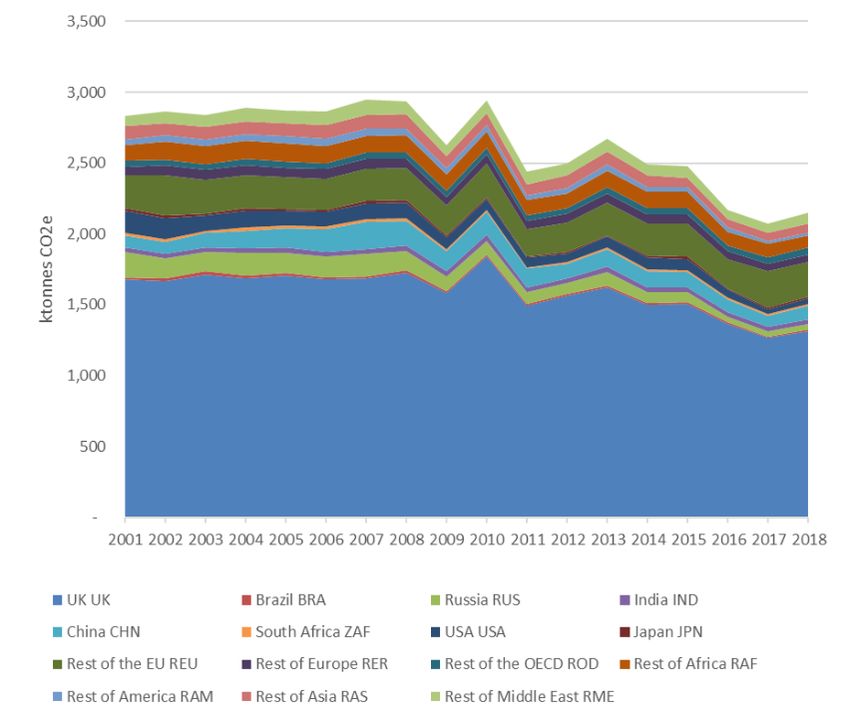
Table 1: Types of emissions inventory included in UK territorial, production and consumption accounts. Green indicated
inclusion and red indicates exclusion. RoW = rest of world

Emissions from… UK UK UK
 Territorial Production Consumption

industries owned by UK, located in UK making products consumed by UK

industries owned by UK, located in UK making products consumed by RoW

industries owned by RoW, located in UK making products consumed by UK

industries owned by RoW, located in UK making products consumed by RoW

industries owned by UK, located in RoW making products consumed by UK

industries owned by UK, located in RoW making products consumed by RoW

industries owned by RoW, located in RoW making products consumed by UK

industries owned by RoW, located in RoW making products consumed by RoW

bunker aviation & shipping owned by UK and used by UK residents

bunker aviation & shipping owned by RoW and used by UK residents

bunker aviation & shipping owned by UK and used by RoW residents

bunker aviation & shipping owned by RoW and used by RoW residents

UK citizens’ activities within UK territory

RoW citizens’ activities within UK territory

UK citizens’ activities within RoW territory

RoW citizens’ activities within RoW territory

land use, land use change and forestry

2.4 Composition of the GHGs
For the 2021 release of the UK consumption-based account we are able to include the full suite of
GHGs as reported to the UNFCCC. These are:

 • Carbon dioxide (CO2)
 • Methane (CH4)
 • Nitrous oxide (N2O)
 • Hydro-fluorocarbons (HFC)
 • Perfluorocarbons (PFC)
 • Nitrogen trifluoride (NF3)
 • Sulphur hexafluoride (SF6) all measured in kilotonnes CO2e

This means that the HCBA for the London Boroughs and the City of London will also contain this full
suite of GHGs.

 4

3 Methodology and data sources
3.1 Overview of the EE-MRIO methodology
Input-output models (IOM) have been adopted by environmental economists due to their ability to
make the link between the environmental impacts associated with production techniques and the
consumers of products. An environmentally-extended multiregional input-output model (EE-MRIO)
uses matrix algebra to transform production-based emissions from industries anywhere in the world
to the point of consumption. This means it is possible to calculate the consumption-based emissions
of nations which take into account the GHGs from full supply chain of production, regardless of where
in the world production stages took place. Once the nation’s CBA is calculated, the emissions
associated with smaller geographies can be determined.

For further detail on the mathematics used in input-output analysis, see the Appendix.

3.2 Data sources
This project will use the University of Leeds’ UKMRIO model (Owen & Barrett, 2020; Owen et al., 2018)
but the data on household final demand for each of the London boroughs and the City of London will
need to be constructed. We need to calculate what proportion of the total London household spend
each of the individual London administrative areas is responsible for, for each consumption item
contained in the database. For example, if households in Harrow spend 30 per cent of the total London
household spend on clothing, it will receive 30 per cent of the total London household footprint
associated with clothing. To understand the portion of London households’ spend by product
attributed to each administrative area we will use two approaches:

Firstly, for domestic consumption of gas and electricity we will use the ‘Regional and local authority
consumption statistics’ produced by BEIS which give estimates of gas and electricity consumption at
the Local Authority level for Great Britain for the years 2005-2019. We will convert the data into
proportions (i.e., what proportion of the total gas and electricity use for London is each administrative
area using) and use trend projections to project the data back to 2001. Home energy use represents
around ¼ of a household’s consumption-based emissions account and so using data on real energy
use is an advantage and will lead to a more accurate estimate of household consumption-based
emissions.

Secondly, for all other consumption, we will construct unique spend profiles using the Living Costs and
Food Survey (LCFS) and the census output area classification (OAC) for each of the 32 London boroughs
and the City of London.

3.3 Using the LCFS and the OAC to construct borough spend profiles
Since 1957, the Office for National Statistics (ONS) has annually surveyed UK households on their
weekly expenditure (UK Data Service, 2019). In 2008 this survey became known as the Living Costs
and Food Survey (LCFS). The LCFS achieves a sample of around 6,000 UK households and is used to
provide information on retail price indices, National Account estimates of household expenditure, the
effect of taxes and benefits, and trends in nutrition. In addition to providing information on household
spend on over 300 different product types (coded by the European Standard Classification of
Individual Consumption by Purpose (COICOP)), further information is collected such as the age, sex
and occupation of members of the household, the total household income, the Government Office
Region they reside in and the household classification of the census output (OAC). The characteristics
of each sampled household are compared to the characteristics of all UK households using the UK
census. The survey strives to produce a representative sample of the 27 million UK households. For
each of the 5000+ household surveys in the 2018 release, a weight is supplied to indicate the

 5

proportion of UK households that are represented by this profile. For example, the 1st household in
the 2018 survey has a weight of 4,576 meaning that 4,567 households in the UK are represented by
this single survey. The sum of every weight is 27 million – the total number of households in the UK.
The LCFS is available in a format that is comparable for the years 2001-2018. This means that results
for the devolved regions and administrative districts below this level start from 2001.

Since the LCFS collects information on the household’s Government Office Region, we can easily
construct a spend profile for all households in London. We then calculate the proportion of spend by
product that London spends compared to the UK total. Multiplying these proportions by total UK
footprint by product disaggregates the consumption-based GHG emissions for the UK down to the
London level. This method ensures that the sum of the regions equals the total footprint. We do not
have locational information on the borough where the surveyed households live, so we cannot simply
follow this method to calculate our borough level HCBAs.

3.3.1 The OAC hierarchy
To construct spend profiles for the London boroughs and the City of London, we use the output area
classification (OAC) data recorded in the LCFS. The OAC is the ONSs’ free and open geodemographic
household segmentation. The OAC provides “summary indications of the social, economic,
demographic, and built characteristics” of the census Output Areas of the UK (Gale et al., 2016, p1).
The OAC is constructed using datasets from the UK Census and there have been two versions of the
classification: one that classifies the 2001 output areas using data from the 2001 census (Vickers &
Rees, 2007) and one which classifies the 2011 output areas using data from the 2011 census (Gale et
al., 2016).

Geodemographic classifications use mathematical clustering algorithms to generate groupings such
that the differences within any group are less than the difference between groups. Once a set of
groups is generated, the creators of the classification system name the individual groups based on
features of the profile and write short “pen portrait” descriptions of them (Gale et al., 2016). Vickers
& Rees (2007, p399) describe the naming process as “difficult and perilous” and note that some names
appear to be contentious, particularly when describing what could be perceived as negative
characteristics. However, Gale et al. (2016, p15) point out that the process “help[s] end users to
identify with the names and description given to local areas” and that the “descriptors had strong and
literal links to the underlying distributions revealed by the data”. The 2001 and 2011 OAC classification
names can be found in the appendix.

Both OACs follow a three-tier classification of supergroups, groups and subgroups (see Table 2). For
example, the 2011 supergroup type 5 is Urbanites, the group type 5a is Urban professionals and
families and the subgroup type 5a3 is Families in terraces and flats.
Table 2: Properties of the 2001 and 2011 OAC

 2001 OAC 2011 OAC
 Number of supergroups 7 8
 Number of groups 21 26
 Number of subgroups 52 76

The LCFS records the 2001 OAC type in the survey years 2008-2013 and the 2011 OAC type in the
survey years 2014-2018. No OAC type is recorded in the LCFS for the years 2001-2007. Using the LCFS,
we generate average spends profiles for each classification type (for the supergroups, groups and
subgroups) by summing the surveys that are characterised by each OAC type and dividing the product

 6

spends by the total weights assigned to these surveys – essentially producing an average spend by
product by household OAC type. We do this for each year to reflect the fact that an OAC type will
change its spend pattern over time. For the years 2001-2007, the spend profiles for 2008 are used as
a proxy. If we know the number of households of each type recorded in each borough, we can produce
a total spend profile for the borough. We then work out the proportion that the borough spends
compared to the total for London. This method ensures that the sum of the boroughs plus the City of
London equals the total footprint of the GLA.

To ensure that the spends captured for the London boroughs truly reflect the character of spends of
London households, rather than use the complete LCFS to generate spend profiles by OAC type, we
first isolate only those surveys found in London. This means that instead of profiling the spend of a
‘3c2 Constrained Commuter’ we are generating the profile of a ‘London 3c2 Constrained Commuter’.
By restricting the surveys to the London surveys, we risk having too few surveys for a representative
sample of households classified as ‘3c2’ (for example). The number of surveys in the LCFS from London
households ranges from 678 in 2001 to 407 in 2014.

To solve the issue of having too few surveys for a representative sample of certain OAC types, we use
a hierarchical decision tree to generate the spend profiles by OAC type. If we take the subgroup
‘London 3c2 Constrained Commuter’ as an example OAC type, if there are 20 or more household
surveys of this type, the average spend for ‘London 3c2’ is recorded. If there are fewer than 20
observations, we move up the classification tree to the group ‘London 3c Ethnic Dynamics’. If there
are 20 or more observations for this type, any households with the classification type 3c2 will be given
the expenditure profile of type 3c. Otherwise, we move to the supergroup ‘London 3 Ethnicity Central’
and follow the same logic. Finally, if there are fewer than 20 observations at the supergroup level, the
households classified as 3c2 would be given the London average spend profile (see Figure 1).

Figure 1: Hierarchical decision tree for assigning spend profiles

Table 3 shows a record of the 2011 OAC subgroups found in Harrow in 2018 and whether the profile
from the subgroup was used or whether it was replaced with a group, supergroup or regional average
spend profile. In the 2018 LCFS there were 25 surveys from households living in London output areas
classified as 3a2 Young families and students and this was deemed to be a sizable sample to create a
spend profile for this subgroup. However, there were only 17 surveys from London households

 7

classified as 3a1 Established renting families. For type 3a1, the group ‘London 3a Ethnic family life’
was used as a proxy spend profile because once we reached this level in the OAC hierarchy, there
were 42 surveys in the 2018 LCFS.
Table 3: Example of the 2011 OAC subgroups found in Harrow in 2018 and the substitution OAC Group or Supergroup used
if needed

 Subgroup OAC name OAC code OAC name used
 Code used
 2a1 Student communal living 2 Cosmopolitans
 2c1 Comfortable cosmopolitan 2 Cosmopolitans
 2d1 Urban cultural mix 2d Aspiring and affluent
 2d3 EU white-collar workers 2d Aspiring and affluent
 3a1 Established renting families 3a Ethnic family life
 3a2 Young families and students 3a2 Young families and students
 3b1 Striving service workers 3b1 Striving service workers
 3b3 Multi-ethnic professional 3b3 Multi-ethnic professional service
 service workers workers
 3c1 Constrained neighbourhoods 3 Ethnicity central
 3d1 New EU tech workers 3d Aspirational techies
 4a3 Commuters with young families 4a3 Commuters with young families
 4b1 Asian terraces and flat 4b1 Asian terraces and flat
 4c1 Achieving minorities 4c Asian traits
 4c2 Multicultural new arrivals 4c2 Multicultural new arrivals
 4c3 Inner city ethnic mix 4c3 Inner city ethnic mix
 5a2 Multi-ethnic professionals with 5a Urban professionals and families
 families
 5a3 Families in terraces and flats 5a Urban professionals and families
 5b1 Delayed retirement 5 Urbanites
 5b2 Communal retirement 5 Urbanites
 6a1 Indian tech achievers 6 Suburbanites
 6b1 Multi-ethnic suburbia 6 Suburbanites

3.3.2 Generating estimates of population by year, OAC and administrative region
Alongside estimates of the spend profiles by OAC types, we need to know how many households are
of each type in each of the London Boroughs and the City of London for each year. 2001 was a Census
year and each of the output areas (OA) in London was classified as one of the 52 different OAC types.
It is possible to record the population and number of households by OA and link the 2001 OAs to
higher level geographies such as the 2018 local authorities (which includes the 32 London boroughs
and the City of London). Similarly, there is population and number of households data for 2011 from
the 2011 Census. The issue is that we need to be able to estimate the population or number of
households by OAC types, by borough, for the years 2002-2010 and 2012-2018.

For the years 2002-2013, it was only possible to find population estimates at the local authority level.
This growth rate in population can be applied to the number of households by OAC from 2001 to
estimate the mix of household types by borough and the City of London. For these years we have to
assume that household occupancy remains stable (the population per households) and we assume
that if the population of a borough grew by 5%, the households classified by each OAC type grew at
exactly the same rate. The mix of OAC types remains in the same proportion as observed in 2001. We

 8

are also assuming that the classification type assigned to an output area (OA) in 2001 is still relevant
in 2013. We assume that the character of the individual OA has not changed.

For the years 2014-2018, population estimates are available at the output area level. This means we
can observe varying growth rates by OAC type since some OAs might grow faster than others within a
borough. However, we are still making the assumption that the classification type assigned in the 2011
census is relevant in 2018. Again, we assume that the character of the individual OA has not changed
and that household occupancies by OAC type are constant over the time period.

Now we have annual estimates of number of households by OAC by borough and annual estimates of
spend by households by OAC type. Multiplying the two together gives a total spend by product by
borough. Table 4 summarises the datasets and methods used to generate the spend profiles for the
boroughs and the City of London. A traffic light system is used to indicate the reliability of the datasets
and methods. It is then a simple step to work out the proportion of the total London spend by product
that each borough is responsible for and apply these proportions to the GLA HCBA to produce the
HCBAs for the 32 boroughs and the City of London.
Table 4: Summary of datasets and methods used to generate spend profiles for the boroughs and the City of London

 OAC OAC spend data Population by OAC type and borough
 classification
 type used
 2001 2001 OAC Take OAC spend Take household figures by OAC from 2001
 proportions from census and sum to borough level
 2008 but match to
 2001 London
 spends
 2002-2007 2001 OAC Take OAC spend Take household figures by OAC from 2001
 proportions from census and sum to borough level. Then use
 2008 but match to ONS dataset 2 on population change by LA
 2002-2007 London level to calculate annual growth rate in
 spends households from a 2001 baseline. Apply this
 same percentage change to each OAC type in
 each LA.
 2008-2013 2001 OAC Annual spend Take household figures by OAC from 2001
 profiles available in census and sum to borough level. Then use
 the LCFS ONS dataset on population change by LA
 level to calculate annual growth rate in
 households from a 2001 baseline. Apply this
 same percentage change to each OAC type in
 each LA.
 2014-2018 2011 OAC Annual spend Take household figures by OAC from 2011
 profiles available in census at the OA level. Use ONS dataset3 on
 the LCFS population change by OA for 2014-2018 to
 estimate number of households by OAC in
 the LAs

2
 MYEB3_summary_components_of_change_series_UK_(2018_geog19).csv. We are aware that the GLA has
their own estimates of population change by London borough which differ from the ONS figures but we aim to
use a national dataset to ensure consistency with other data from the ONS and to match the population data
used from the ONS from 2014-2018
3
 mid-2014-2018-coa-unformatted-syoa-estimates-london.xlsx

 9

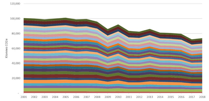
4 Results
4.1 High level results
The household consumption-based account for London has decreased from 101 Mtonnes CO2e in
2001 to 74 Mtonnes CO2e in 2018 – a reduction of 27 per cent (Figure 2). Note there is no key as this
chart is illustrative of the overall pattern. This reduction is in line with reductions seen at a national
level and is mainly due to decarbonisation of the electricity sector reducing the emissions intensity of
products bought. Some of the reduction is due to reduced spend post-recession and an increased
reliance on domestically produced goods rather than imports post-recession.

Figure 2: Cumulative HCBA for all London boroughs and the City of London

Every London borough has seen a reduction in their total HCBA with Kensington and Chelsea reducing
by the largest proportion (37.2 per cent) and Tower Hamlets reducing by the smallest (7.5 per cent),
starting from a relatively high and relatively low base to start with (see Figure 3a).

London has seen population growth in the period 2001-2018. On a per capita basis, which takes
account of population changes within London, the reductions are even more significant. Newham has
seen the largest reduction (44.0 per cent) and Tower Hamlets the least (31.8 per cent) (see Figure 3b).

 10

Figure 3a: Percentage change in total HCBA for all London boroughs and the City of London between 2001 and 2018

Figure 4b: Percentage change in per capita HCBA for all London boroughs and the City of London between 2001 and 2018

In addition to seeing overall reductions in HCBA GHG emissions per capita, the variation in impact has
reduced over the time-period with a standard deviation of 1.55 tonnes in 2001 and 0.94 tonnes in
2018 (Table 5).
Table 5: Summary statistics for 2001 and 2018

 2001 2018
 Max (tonnes CO2e per capita) 17.33 (City of London) 11.22 (City of London)
 Min 10.27 (Tower Hamlets) 6.03 (Newham)
 Standard deviation 1.55 0.94

 11

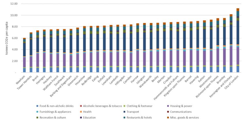
The breakdown of HCBA by high level product groups is similar for all boroughs in 2018 (Figure ). In every borough, the item with the largest impact is
transport, followed by housing and power. Transport has the largest range (1.83 tonnes) in per capita HCBA, ranging from 4.15 tonnes in the City of London
to 2.32 in Newham. The range (1.63 tonnes) of values for housing and power is between 3.35 tonnes in Kensington and Chelsea and 1.73 tonnes in Newham.
Please see the Appendix for information as to what is contain in each product group.

In London, food and drink makes up 10.9 per cent of an average household CBA. In the wealthier areas of the City of London and Kensington and Chelsea this
proportion is slightly smaller (9.9 per cent and 9.6 per cent respectively). We see a greater proportion of impact associated with restaurants and hotels in the
City of London (8.1per cent) compared to the average (7.0 per cent). In general, the wealthy areas have larger than average impacts, driven by spends on
goods such as clothing, air travel, recreation and other services.

Figure 4: Breakdown of HCBA per capita by high level consumption items for all London Boroughs and the City of London (2018)

 12

4.2 Guide to using the individual borough level datasets
An Excel dataset has been produced for each of the 32 London Boroughs and the City of London. The
first sheet (see Figure 5) is a menu of the type of data that can be viewed for the specific local area.

Figure 5: The overview sheet in the borough level dataset

The remainder of the dataset is as follows:

 1. Dashboard – this is a summary sheet showing headline results for the borough
 2. Total emissions by source region (2001-2018) – this is the total HCBA broken down by the
 region of origin of the emissions
 3. Emissions by detailed COICOP classification (2001-2018) – this shows the total emissions at
 the most detailed level or 307 different COICOP products
 4. Emissions per capita by detailed COICOP classification (2001-2018) – this is the same as (3)
 but divided by population to show per capita emissions
 5. Emissions by aggregated product group (2001-2018) – the emissions by 12 high-level
 product groups
 6. Emissions by source industry (2001-2018) – this is the HCBA broken down by the industry of
 origin of the emissions
 7. Emissions by GHG protocol (2001-2018) – this is the HCBA broken down by scopes 1, 2 and 3
 8. Index chart by product group (2001-2018) – chart showing relative change from 2001 of the
 12 high-level product groups
 9. Comparison with region and UK by product (2001-2018) – sheet showing 12 per capita HCBA
 charts for each of the high-level product groups, for the borough, GLA and UK
 10. Start of the datasheets – the core datasheets that are used to construct the previous 9
 sheets start from this point

In the following sections we deep dive into the results of Harrow as an example of how to interpret
the data.

 13

4.2.1 Total and per capita emissions time series
The first two charts on the dashboard show the time series of total household consumption-based
emissions for Harrow and a comparison of the per capita emissions with London as a whole and the
whole of the UK. Comparing the blue line for Harrow on Figure 6 and Figure 7 reveals how population
growth effects the emissions estimate and that the per capita reduction is steeper. Harrow has a larger
than average HCBA compared to London as a whole and the UK. Most of the reduction in emissions
occurred between 2008 and 2011 and 2015 and 2016. Country-wide, we see large reductions in
emissions during the 2007-2009 recession and more recently due to decarbonisation of the electricity
sector.

Figure 6: Total emissions from households for Harrow 2001-2018

Figure 7: Per capita household emission for Harrow, London and the UK 2001-2018

 14

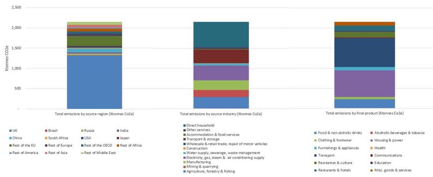
4.2.2 Emissions breakdown by source and final product
The third chart (Figure 8) on the dashboard shows the total household CBA for Harrow broken down in three different ways:

 • Where in the world the emissions were released to meet consumption by Harrow residents?
 • Which industries were responsible for these emissions?
 • Which final products are the emissions embodied in?

Figure 8: Breakdown of total Harrow HCBA by source and final product (2018)

The greatest proportion (61.1per cent) of emissions associated with Harrow household’s consumption are released in the UK. This is due to the large
proportion of consumption associated with home heating and personal transport. A further 11.6 per cent are emissions from the EU. The UK imports many
products from the continent, particularly agriculture. 29.2 per cent of Harrow’s household consumption emissions are direct household emissions from

 15

burning fuel in the home and personal transport. A further 17.1 per cent can be traced back to the
production of electricity used both in the home and in the supply chain of other goods. The final
stacked bar in Figure 8 is the same breakdown shown in Figure 4. These type of breakdown charts can
be useful in order to understand where emissions reduction policy should focus.

 For example, in Harrow, policy makers may consider targeting emissions from the three largest
consumption areas: transport, housing & power and food & non-alcoholic drinks. The breakdown
shows that targeting emissions associated with household spend on education will not be associated
with large reduction

4.2.3 Product based comparisons with the UK and London
Figure 9 allows the user to compare the average levels of consumption in the borough with averages
for the whole of the UK and the whole of London. The chart is a propensity chart with the UK and
London set at 100 and the borough level is compared to this index level. For example, Harrow has a
level of 82 for furnishing and appliances meaning that the average household in Harrow spends 82 per
cent of the UK average for this product type and consequently has a lower-than-average impact for
this category of spend. For recreation and culture, Harrow has a level of 153 compared to London,
meaning that residents of Harrow spend and have an impact 53 per cent higher than the average
London resident for this category of spend.

Figure 9: Product based comparisons for Harrow with the UK and London (2018)

This type of data can be useful in understanding why a borough has a lower or higher than average
impact compared to London or the UK. Harrow has a higher-than-average impact for housing and
power. The policy maker may want to investigate if this could be due to a less-than-average efficiency
of housing stock.

 16

4.2.4 Ranked comparisons with the rest of London
The next few charts in the dashboard compare total and per capita results for Harrow with the other
London boroughs and the City of London. The borough of Harrow is highlighted in red.

Figure 10: Per capita results comparing the borough of Harrow with the other London boroughs and the City of London (2018)

Ranked charts can be useful when comparing two boroughs with similar characteristics but different
household emissions profiles. Are there two boroughs with similar levels of wealth but very different
housing and power impacts? Comparing the borough rankings over time might reveal information
about how some areas have changed and some have not.

 17

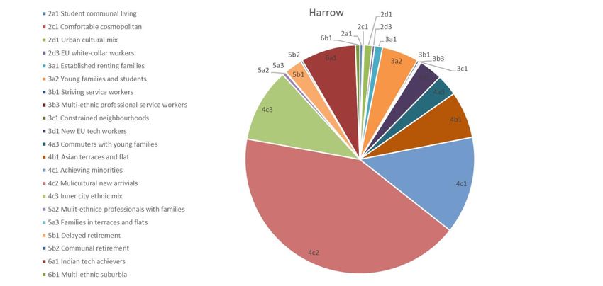
4.2.5 Breakdown of OAC subgroups
The final chart on the dashboard shows the make-up of OAC subgroups in the borough. In 2018, there are an estimated 105,599 residents living in output
areas classified as type 4c2 Multicultural new arrivals. This is the largest group (42.2per cent), followed by 4c1, achieving minorities and 4c3, inner city ethnic
mix.

Figure 11: OAC subgroups in Harrow by population (2018)

In the ‘backend’ of the spreadsheet you can find further information about the OAC for earlier years. Sheets in the format ‘ghg_year_oac’ show the population
by OAC type and the higher level OAC substitutions made where this was necessary.

 18

4.2.6 Source region time series
The next sheet in the dataset, shows the breakdown by source region for the entire timeseries.

Figure 12: Breakdown of total HCBA for Harrow by source region (2001-2018)

In 2001, imported emissions contributed 40.8 per cent of the total HCBA, compared to 38.9 per cent
in 2018. Post-recession, imported emissions reduced by a greater proportion than domestic emissions
because households reduced expenditure on consumables by a greater amount than spend on
heating, power and local transportation where emissions are predominantly domestic.

4.2.7 Further detailed breakdowns by year, product, industry and scope
Sheets 3 and 4 show the most detailed breakdown of the results by total and by per capita. At the
most detailed level, borough results can be viewed by 307 product types. However, it is not
recommended that results are used at this level. As a general rule, the more granular the results, the
less accurate the numbers are. Due to the way the UKMRIO database is constructed, although there
is information about the spend levels by 307 product groups, by the different OAC types, the CO2e
conversion factors operate best at a more aggregated level. Many of the product types have the same
conversion factor because the model can only determine a conversion factor for clothing, for example
not at the level of ‘womens’ under garments’. It is recommended that the 12 product types shown in
previous figures are adopted for reporting purposes. However, if the user wants to understand the
portion of the transport impact that is passenger travel by air, for example, sheets 3 and 4 can help
disaggregate the results for this type of analysis.

Sheet 6 breaks down the emissions by year and 114 source industries and sheet 7 reclassifies the
emissions to fit the Scope 1, 2 and 3 categories used in the GHG protocol.
 19

4.2.8 Product-based time-series comparisons and a note on noise in the data
Sheet 9 reveals how the per capita impact for the borough has changed over time for each of the 12
high-level product groups. A comparison with the London and UK averages is also shown. Figure 13
shows that Harrow’s food and drink impact per capita is lower than the UK average and similar to that
of London.

Figure 13: Per capita food and non-alcoholic drinks HCBA for Harrow, London and UK (2001-2018)

Note that the UK data is a relatively smooth line, whereas London, then the borough get progressively
more jagged. A more extreme example of this can be seen in Figure 14, the health impact chart, where
there is a significant spike in 2007.

Figure 14: Per capita health HCBA for Harrow, London and UK (2001-2018)

 20

This irregularity or noise further demonstrates how the aggregated data is more accurate than the
disaggregated values. The UK trend for health is smooth and it gets more erratic, the smaller the
geography. The reason for this is that health expenditure in the LCFS is a sporadic spend – not
something that every household spends money on every week. In 2007, London households were
disproportionately captured as spending a larger than average share of the total UK spend on private
health services and those OAC type that spent on this category were concentrated in Harrow, meaning
the spike appears even larger. With this type of sporadic spend item, we recommend considering a
‘line of best fit’ approach to the footprint, viewing the overall trend (slight reduction) rather than
giving too much importance to individual years’ values.

Fortunately, the consumption items that are most important in a household account are items that
are bought frequently (food, fuel, transportation) and do not suffer from noise in the data due to
sporadic spend. The expenditure categories where the consumption impact is erratic have a very low
overall impact.

4.2.9 Advanced level analysis
Further sheets in the back end of the spreadsheet allow for further breakdown of the results. For
example, sheet ‘ghg_2001_reg’ shows the source emission region by product type in the year 2001.
Here you can determine that three quarters of the emissions associated with household appliances
are imported, for example. Or sheet ‘ghg_2018_ind’ can be used to show the source industries
associated with each product. Here you can predict how each product may reduce its impact if the
emissions associated with ‘electric power generation’ were zero.

 21

5 Conclusions, recommendations and next steps
5.1 Overall findings
The University of Leeds has successfully developed a robust and replicable methodology to calculate
the household consumption-based GHG account of all 32 London Boroughs and the City of London.
The results show that household consumption emissions have reduced significantly across all
boroughs in the period 2001-2018. However further action is needed to reach targets at the borough,
region and national level. We find that major areas of consumption are broadly consistent across
boroughs – emissions from transport, housing & power and food represent the majority of a HCBA.
There is some variation across the boroughs with the richest boroughs having the highest impact for
non-essential consumption items like hotels and restaurant spend. We have recommended caution in
using results at the more granular levels where there is potential for noise in the data but we are
confident that the overall trends accurately indicate the direction of travel in emissions.

The results presented provide an important borough level picture for how boroughs and the region
can focus efforts to reduce emissions in line with adopted targets.

5.2 Comment on methodology, data sources and update potential
The methodology used ensures that the sum of the London boroughs plus the City of London equals
the reported HCBA for the GLA. The data used to disaggregate the GLA’s HCBA to the individual
borough level is free, open source and annually updated. Now that the methodology has been
established, updating the dataset for 2019 should be a relatively straight forward process. The
UKMRIO database will be updated in early 2022 and will be capable of reporting the UK CBA for 1990-
2019. This data will be published in Spring 2022 alongside the GLA CBA for 2001-2019. Once this data
is published, the 2019 borough and City of London results could be processed.

2021 is a census year, which means there will be a new 2021 Output Area Classification and any
changes to an area’s character can be reflected. It takes a number of years for the census to be
processed and for a new OAC to be finalised. It is unlikely that we will see a 2021 OAC reflected in the
LCFS until 2024. In addition, the UKMRIO database is always 3 years out of date due to the time it
takes to update the National Accounts. This means that we will not see the effects of a new OAC until
publication of 2024 in 2027.

It is important to note that the underlying model, the UKMRIO database, is completely updated each
year and the entire time series is re-estimated to reflect any updates to data sources and
methodological improvements. This means that results for 2001-2018 may be re-estimated in 2022
and change slightly. This will affect the London borough HCBA and it is recommended that the entire
time series is re-estimated each year, rather than simply reporting the next additional year.

5.3 Recommendation for wider coverage
This project has demonstrated that it is possible to disaggregate HCBA for the UK regions down to the
local authority level. The data used for the London boroughs is available for all the other regions in
England and for the devolved nation of Wales. This means it would be simple to produce results
datasheets for all local authorities in England and Wales. Scottish census data is recorded slightly
differently but we are confident that this methodology could also be applied to the Scottish Local
Authorities. The OAC is not recorded for Northern Irish households in the LCFS so an alternate
approach would need to be developed to disaggregate HCBA in Northern Ireland.

London Councils has led the way in commissioning data on consumption-based emissions accounts
for the boroughs and the City of London. As accounting for emissions from consumption continues to

 22

move up the political agenda, and the UK starts to consider how to develop targets for consumption
emissions reductions, it is likely that more and more local councils will request consumption-based
emissions estimates. These results will only be meaningful if developed in a manner consistent with
the national level results. We strongly recommend that this London case study becomes the blueprint
for the rest of the country.

 23

6 References
Davis, S. J., & Caldeira, K. (2010). Consumption-based accounting of CO2 emissions. Proceedings of
 the National Academy of Sciences, 107(12), 5687–92. doi:10.1073/pnas.0906974107
Gale, C. G., Singleton, A. D., Bates, A. G., & Longley, P. A. (2016). Creating the 2011 area classification
 for output areas (2011 OAC). Journal of Spatial Information Science, 12(2016), 1–27.
 doi:10.5311/JOSIS.2016.12.232
Hertwich, E. G., & Peters, G. P. (2008). Policy Analysis CO 2 Embodied in International Trade with
 Implications for Global Climate Policy. Environmental Science & Technology, 42(5), 1401–1407.
 doi:10.1021/es072023k
IPCC. (2007). Climate Change 2007 : An Assessment of the Intergovernmental Panel on Climate
 Change. Synthesis Report, (November), 12–17.
Kitzes, J. (2013). An Introduction to Environmentally-Extended Input-Output Analysis. Resources, 2,
 489–503. doi:10.3390/resources2040489
Miller, R. E., & Blair, P. D. (2009). Input-output analysis: foundations and extensions. Cambridge
 University Press.
Owen, A., & Barrett, J. (2019). Consumption based Greenhouse Gas Emissions for London. Retrieved
 from https://www.london.gov.uk/sites/default/files/final_report_-
 _consumption_ghg_accounts_for_london_-_for_publication.pdf
Owen, A., & Barrett, J. (2020). Reducing inequality resulting from UK low-carbon policy. Climate
 Policy, 20(10), 1193–1208. doi:10.1080/14693062.2020.1773754
Owen, A., Scott, K., & Barrett, J. (2018). Identifying critical supply chains and final products: An input-
 output approach to exploring the energy-water-food nexus. Applied Energy, 210, 632–642.
 doi:10.1016/j.apenergy.2017.09.069
Peters, G. P., Andrew, R., & Lennox, J. (2011). Constructing an Environmentally-Extended Multi-
 Regional Input–Output Table Using the Gtap Database. Economic Systems Research, 23(2),
 131–152. doi:10.1080/09535314.2011.563234
UK Data Service. (2019). Living Costs and Food Survey.
UK Government. (2021). UK’s Carbon Footprint. Retrieved May 5, 2021, from
 https://www.gov.uk/government/statistics/uks-carbon-footprint
Vickers, D., & Rees, P. (2007). Creating the UK National Statistics 2001 output area classification.
 Journal of the Royal Statistical Society. Series A: Statistics in Society, 170(2), 379–403.
 doi:10.1111/j.1467-985X.2007.00466.x
Wiedmann, T. (2009). A review of recent multi-region input–output models used for consumption-
 based emission and resource accounting. Ecological Economics, 69(2), 211–222.
 doi:10.1016/j.ecolecon.2009.08.026

 24

7 Appendix
7.1 Input-output analysis
The Leontief Input-Output model is constructed from observed economic data and shows the
interrelationships between industries that both produce goods (outputs) and consume goods (inputs)
from other industries in the process of making their own product (Miller & Blair, 2009).

 Purchases from intermediate
 demand

 Zaa Zab yac
 Sales to Intermediate

 Total Output (x)
 Sales to
 Transaction Matrix
 demand

 Final
 (Z) Demand
 (Y)
 Zbb ybd

 Value Added (H)

 Total Input (x)

 Environmental Extensions (F)
Figure 15: Basic structure of a Leontief Input-Output Model

Consider the transaction matrix Z; reading across a row reveals which industries a single industry sells
to and reading down a column reveals who a single industry buys from. A single element, zij, within Z,
represents the contributions from the ith sector to the jth industry or sector in an economy. For
example, represents the ferrous metal contribution in making ferrous metal products, , the
ferrous metal contribution to car products and the car production used in making cars. Final
demand is the spend on finished goods. For example, is the spend on ferrous metal products by
households as final consumers whereas is the spend on car products by government as final
consumers.

The total output (xi) of a particular sector can be expressed as:

 = + + ⋯ + + (1)

where yi is the final demand for that product produced by the particular sector. If each element, zij,
along row i is divided by the output xi , associated with the corresponding column j it is found in, then
each element in Z can be replaced with:
 
 = 
 (2)

to form a new matrix .

Substituting for (2) in equation (1) forms:

 = + + ⋯ + + (3)

Which, if written in matrix notation is = + . Solving for gives:

 25

 = ( − )− (4)

where and are vectors of total output and final demand, respectively, is the identity matrix, and
 is the technical coefficient matrix, which shows the inter-industry requirements. ( − )− is
known as the Leontief inverse (further identified as ). It indicates the inter-industry requirements of
the ith sector to deliver a unit of output to final demand. Since the 1960s, the IO framework has been
extended to account for increases in the pollution associated with industrial production due to a
change in final demand (Kitzes, 2013).

Consider, a row vector of annual GHG emissions generated by each industrial sector

 = ̂ − (5)

is the coefficient vector representing emissions per unit of output4. Multiplying both sides of (4) by
 ′ gives

 ′ = ′ (6)

and simplifies to

 = ′ (7)

where is the GHG emissions in matrix form allowing consumption-based emissions to be
determined. is calculated by pre-multiplying by emissions per unit of output and post-multiplying
by final demand. This system can be expanded to the global scale by considering trade flows between
every industrial sector in the world rather than within a single country. This type of system requires a
multi-regional input –output (MRIO) table (Peters et al., 2011).

To calculate the emissions associated with a subset of the total region, the final demand vector is
replaced with the final demand corresponding to the area of focus. For example, if the final demand
vector _ is used which shows final demand by product for households in Harrow, the
calculation = ′ _ will give the consumption-based account for Harrow’s households

7.2 Output area classifications for 2001 and 2011
Table 6: 2001 OAC Supergroups

 Supergroup name
 1 Blue Collar Communities
 2 City Living
 3 Countryside
 4 Prospering Suburbs
 5 Constrained by Circumstances
 6 Typical Traits
 7 Multicultural

Table 7: 2001 OAC Groups

 Group name
 1a Terraced Blue Collar
 1b Younger Blue Collar

4 ̂ denotes matrix diagonalisation and ′ denotes matrix transposition

 26

1c Older Blue Collar
 2a Transient Communities
 2b Settled in the City
 3a Village Life
 3b Agricultural
 3c Accessible Countryside
 4a Prospering Younger Families
 4b Prospering Older Families
 4c Prospering Semis
 4d Thriving Suburbs
 5a Senior Communities
 5b Older Workers
 5c Public Housing
 6a Settled Households
 6b Least Divergent
 6c Young Families in Terraced Homes
 6d Aspiring Households
 7a Asian Communities
 7b Afro-Caribbean Communities

Table 8L 2001 OAC Subgroups

 Subgroup name
 1a1 Terraced Blue Collar 1
 1a2 Terraced Blue Collar 2
 1a3 Terraced Blue Collar 3
 1b1 Younger Blue Collar 1
 1b2 Younger Blue Collar 2
 1c1 Older Blue Collar 1
 1c2 Older Blue Collar 2
 1c3 Older Blue Collar 3
 2a1 Transient Communities 1
 2a2 Transient Communities 2
 2b1 Settled in the City 1
 2b2 Settled in the City 2
 3a1 Village Life 1
 3a2 Village Life 2
 3b1 Agricultural 1
 3b2 Agricultural 2
 3c1 Accessible Countryside 1
 3c2 Accessible Countryside 2
 4a1 Prospering Younger Families 1
 4a2 Prospering Younger Families 2
 4b1 Prospering Older Families 1
 4b2 Prospering Older Families 2
 4b3 Prospering Older Families 3
 4b4 Prospering Older Families 4
 4c1 Prospering Semis 1
 4c2 Prospering Semis 2

 27

4c3 Prospering Semis 3
 4d1 Thriving Suburbs 1
 4d2 Thriving Suburbs 2
 5a1 Senior Communities 1
 5a2 Senior Communities 2
 5b1 Older Workers 1
 5b2 Older Workers 2
 5b3 Older Workers 3
 5b4 Older Workers 4
 5c1 Public Housing 1
 5c2 Public Housing 2
 5c3 Public Housing 3
 6a1 Settled Households 1
 6a2 Settled Households 2
 6b1 Least Divergent 1
 6b2 Least Divergent 2
 6b3 Least Divergent 3
 6c1 Young Families in Terraced Homes 1
 6c2 Young Families in Terraced Homes 2
 6d1 Aspiring Households 1
 6d2 Aspiring Households 2
 7a1 Asian Communities 1
 7a2 Asian Communities 2
 7a3 Asian Communities 3
 7b1 Afro-Caribbean Communities 1
 7b2 Afro-Caribbean Communities 2

Table 9: 2011 OAC Supergroups

 Supergroup name
 1 Rural residents
 2 Cosmopolitans
 3 Ethnicity central
 4 Multicultural metropolitans
 5 Urbanites
 6 Suburbanites
 7 Constrained city dwellers
 8 Hard-pressed living

Table 10: 2011 OAC Groups

 Group name
 1a Farming communities
 1b Rural tenants
 1c Aging rural dwellers
 2a Students around campus
 2b Inner city students
 2c Comfortable cosmopolitan
 2d Aspiring and affluent

 28

3a Ethnic family life
 3b Endeavouring Ethnic Mix
 3c Ethnic dynamics
 3d Aspirational techies
 4a Rented family living
 4b Challenged Asian terraces
 4c Asian traits
 5a Urban professionals and families
 5b Ageing urban living
 6a Suburban achievers
 6b Semi-detached suburbia
 7a Challenged diversity
 7b Constrained flat dwellers
 7c White communities
 7d Ageing city dwellers
 8a Industrious communities
 8b Challenged terraced workers
 8c Hard pressed ageing workers
 8d Migration and churn

Table 11L 2011 OAC Subgroups

 Subgroup name
 1a1 Rural workers and families
 1a2 Established farming communities
 1a3 Agricultural communities
 1a4 Older farming communities
 1b1 Rural life
 1b2 Rural white-collar workers
 1b3 Aging rural flat tenants
 1c1 Rural employment and retirees
 1c2 Renting rural retirement
 1c3 Detached rural retirement
 2a1 Student communal living
 2a2 Student digs
 2a3 Students and professionals
 2b1 Students and commuters
 2b2 Multicultural student neighbourhoods
 2c1 Comfortable cosmopolitan
 2c2 Migrant commuters
 2c3 Professional service cosmopolitans
 2d1 Urban cultural mix
 2d2 Highly-qualified quaternary workers
 2d3 EU white-collar workers
 3a1 Established renting families
 3a2 Young families and students
 3b1 Striving service workers
 3b2 Bangladeshi mixed employment
 3b3 Multi-ethnic professional service workers

 29

3c1 Constrained neighbourhoods
3c2 Constrained commuters
3d1 New EU tech workers
3d2 Established tech workers
3d3 Old EU tech workers
4a1 Social renting young families
4a2 Private renting new arrivals
4a3 Commuters with young families
4b1 Asian terraces and flat
4b2 Pakistani communities
4c1 Achieving minorities
4c2 Multicultural new arrivals
4c3 Inner city ethnic mix
5a1 White professionals
5a2 Multi-ethnic professionals with families
5a3 Families in terraces and flats
5b1 Delayed retirement
5b2 Communal retirement
5b3 Self-sufficient retirement
6a1 Indian tech achievers
6a2 Comfortable suburbia
6a3 Detached retirement living
6a4 Ageing in suburbia
6b1 Multi-ethnic suburbia
6b2 White suburban communities
6b3 Semi-detached ageing
6b4 Older workers and retirement
7a1 Transitional Eastern European neighbourhoods
7a2 Hampered aspiration
7a3 Multi-ethnic hardship
7b1 Eastern European communities
7b2 Deprived neighbourhoods
7b3 Endeavouring flat dwellers
7c1 Challenged transitionaries
7c2 Constrained young families
7c3 Outer city hardship
7d1 Ageing communities and families
7d2 Retired independent city dwellers
7d3 Retired communal city dwellers
7d4 Retired city hardship
8a1 Industrious transitions
8a2 Industrious hardship
8b1 Deprived blue-collar terraces
8b2 Hard pressed rented terraces
8c1 Ageing industrious workers
8c2 Ageing rural industry workers
8c3 Renting hard-pressed workers
8d1 Young hard-pressed families
8d2 Hard-pressed ethnic mix
8d3 Hard-pressed European Settlers

 30