HETEROGENEOUS IMPACT OF MERCOSUR 2021 - Documentos de Trabajo N.º 2114 Rodolfo G. Campos and Jacopo Timini - Banco de España
←
→
Page content transcription
If your browser does not render page correctly, please read the page content below
UNEQUAL TRADE, UNEQUAL GAINS: THE
HETEROGENEOUS IMPACT OF MERCOSUR
                                      2021

Documentos de Trabajo
N.º 2114

Rodolfo G. Campos and Jacopo Timini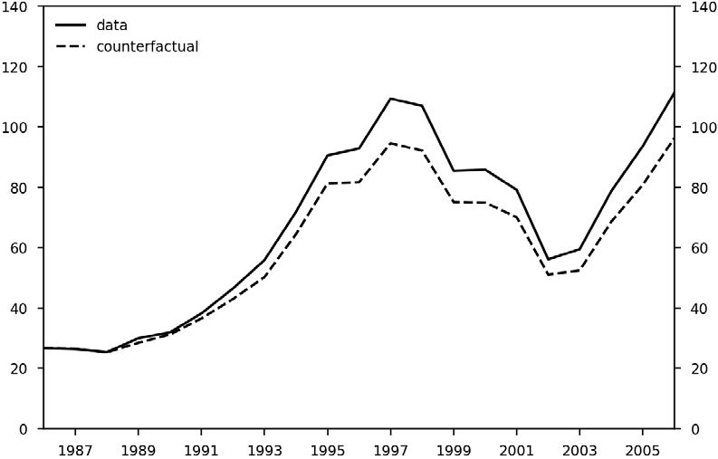
UNEQUAL TRADE, UNEQUAL GAINS: THE HETEROGENEOUS IMPACT
OF MERCOSUR
UNEQUAL TRADE, UNEQUAL GAINS: THE HETEROGENEOUS
IMPACT OF MERCOSUR (*)

Rodolfo G. Campos and Jacopo Timini
BANCO DE ESPAÑA

(*) In writing this paper we have benefited from the discussion by Francisco Requena Silvente at the XVII Workshop
on Economic Integration (Valencia), and from comments and suggestions by Pedro del Río, an anonymous referee
(Banco de España working paper series), and seminar participants at Banco de España and at the FREE seminar.
The views expressed in this paper are those of the authors and do therefore not necessarily reflect those of the
Banco de España or the Eurosystem.

Documentos de Trabajo. N.º 2114
March 2021
The Working Paper Series seeks to disseminate original research in economics and finance. All papers
have been anonymously refereed. By publishing these papers, the Banco de España aims to contribute
to economic analysis and, in particular, to knowledge of the Spanish economy and its international
environment.

The opinions and analyses in the Working Paper Series are the responsibility of the authors and, therefore,
do not necessarily coincide with those of the Banco de España or the Eurosystem.

The Banco de España disseminates its main reports and most of its publications via the Internet at the
following website: http://www.bde.es.

Reproduction for educational and non-commercial purposes is permitted provided that the source is
acknowledged.

© BANCO DE ESPAÑA, Madrid, 2021

ISSN: 1579-8666 (on line)
Abstract

We estimate the impact of MERCOSUR on trade flows and on gains from trade for its
member countries using a standard modern general equilibrium quantitative structural
gravity model. We find a highly heterogeneous impact on bilateral trade flows and gains
from trade. We estimate that gains from trade attributable to MERCOSUR are equivalent
to a 4.0 % increase in per-capita consumption for Argentina. For the other countries,
gains from trade are smaller: 0.8 % for Uruguay, 0.5 % for Paraguay, and 0.3 % for Brazil.
We study whether Brazil would benefit from withdrawing from MERCOSUR and signing
a trade agreement with a different trade bloc but conclude that net gains from such a
switch would be small, if any.

Keywords: general equilibrium, international trade, MERCOSUR, structural gravity
model, trade agreements.

JEL classification: F13, F14, F15, F62.
Resumen

Este artículo estima el impacto del MERCOSUR sobre los flujos comerciales y el
bienestar usando un modelo de gravedad estructural cuantitativo estándar. El impacto
sobre los flujos de comercio bilateral y sobre el bienestar es altamente heterogéneo
entre los países del MERCOSUR. El aumento de bienestar atribuible al MERCOSUR
equivale a un incremento del 4,0 % del consumo per cápita en el caso de Argentina,
mientras que para los otros integrantes del acuerdo el efecto es inferior: el 0,8 % en el
caso de Uruguay, el 0,5 % en Paraguay y el 0,3 % en Brasil. Un cálculo estimativo del
efecto sobre el bienestar para Brasil de abandonar el MERCOSUR, y firmar un acuerdo
con otro bloque comercial, arroja un resultado neto muy reducido o incluso nulo.

Palabras clave: equilibrio general, comercio internacional, MERCOSUR, modelo de
gravedad estructural, tratados de comercio.

Códigos JEL: F13, F14, F15, F62.
1       Introduction

          Countries do not benefit equally from signing a trade agreement. Recent research (e.g., Kohl,
          2014; Baier et al., 2019b; El Dahrawy Sánchez-Albornoz and Timini, 2020) reports estimates
          of the impact of trade agreements on trade flows that differ widely, both between and within
          trade agreements. Usually, welfare gains from trade also differ substantially between trade
          partners, possibly leading to conflict within a trade bloc, or ex-post renegotiation attempts
          by countries that sign a trade agreement. In this paper we study mercosur, a trade bloc
          established by Argentina, Brazil, Paraguay and Uruguay in 1991, and estimate the impact on
          trade and welfare for its members within a structural gravity model framework, using modern
          methods, and allowing for heterogeneity within the trade bloc.

          Mercosur serves as an interesting case study for various reasons. First, countries are of very
          different sizes, a circumstance that is likely to lead to heterogeneity in trade flows and in gains
          from trade. Second, as with other trade blocs, some of its members have occasionally flirted
          with abandoning the trade bloc, and our estimates will serve to compute the impact on welfare
          of such a move.1 Third, although mercosur has received a moderate amount of attention in the
          past, it has not been studied to the same extent as the European Union or the North American
          Free Trade Agreement (nafta); in particular, the study of this particular trade bloc—the
          fourth largest in the world—lags behind in the use of the most recent methodological advances.
          To our knowledge, ours is the first paper to study the impact of mercosur specifically using a
          modern medium-sized quantitative structural gravity model and data on intra-national trade
          flows that are constructed in a consistent way.2

          To draw conclusions that are unencumbered by specific model details, we employ a general
          structural gravity framework that encompasses a large set of individual models that have been
          proposed to explain bilateral trade flows in the past. After estimating the parameters of the
          model in a theory-consistent way, we calculate gains from trade in general equilibrium using a
          sufficient statistics formula à la Arkolakis et al. (2012), which requires information on just two
          sufficient statistics: the change in the share of internal trade and an elasticity parameter. This
          implies that our results on welfare do not depend on the exact details of an underlying model,
          as long as it fits into the structural gravity framework, as defined by Head and Mayer (2014).

          We find that mercosur has had a very heterogeneous impact on trade flows between its
          members. Argentina plays a central role, with trade flows attributed to mercosur into and
          out of Argentina rising more than for the other trade relationships within the bloc. In fact,
          the bilateral trade flows between Argentina and Brazil strengthened substantially, as did trade
          flows between other bloc members and Argentina—but not between other bloc members and
          Brazil. These results explain why we find the largest gains from trade for Argentina.

         Brazil is the member of mercosur with the lowest gains from trade. This begs the question of
         whether Brazil would be better off by withdrawing from the agreement and joining a different
         trade bloc. We explore this question through a series of counterfactual scenarios and find that

              1
               Newspaper coverage on countries’ threats to withdraw from mercosur is abundant, for example, The
          Economist (2012), Preissler Iglesias and Gamarski (2019), and Nessi (2020).
             2
               Intra-national trade flows are desirable for theoretical reasons in a structural gravity model and, in our case,
          they are a necessary input to calculate effects on welfare.

BANCO DE ESPAÑA   7   DOCUMENTO DE TRABAJO N.º 2114
gains from trade for Brazil of switching into other trade agreements would be small, and therefore
likely to be outweighed by switching costs associated to exiting the old treaty (e.g., increased
uncertainty, disruptions in global and regional value chains) or entering the new one (use of
political capital for negotiations and approval of the treaty), other economic factors (economic
benefits from further integration within mercosur) and domestic considerations distinct from
gains from trade (e.g., the democratic clause or the migratory regulations embedded in the
mercosur treaty).
Prior work that has studied the impact of mercosur on trade flows within a structural gravity
framework consistently finds that mercosur has led to an increase of intra-bloc trade. For
example, Baier et al. (2007) report a large positive impact on trade flows and Magee (2008)
and Baier et al. (2018) find that the impact of mercosur on trade flows exceeds that of other
regional trade agreements.3 Closer to our work is the recent paper by Baier et al. (2019b),
which estimates a structural gravity model allowing for heterogeneous impacts on trade bloc
members, and using data that include intra-national trade flows. It finds that the trade impact
of mercosur is on the high end of the distribution of regional trade agreements.4
Our empirical strategy differs from prior work in that we employ more flexible specifications
to explore whether the impact of mercosur changes over time, or is heterogeneous between
mercosur members, and that we also focus on gains from trade. We proceed in two steps.
In a first step we use a specification in which mercosur is allowed to have a fully flexible
impact on trade costs and trade flows along the temporal dimension. The results from this first
part confirm historical details known about mercosur and show a distinction between two
periods: a transitional period between 1991 and 1994 with a rising impact on trade flows and a
second period that starts in 1995 during which the impact on trade settles at a higher level. In
a second step, we study heterogeneity between bloc members in each of these two periods.
A paper that comes close in spirit to our general question and to our focus on the computation of
gains from trade is a recent article by Baier et al. (2019a), who study the impact of a hypothetical
dissolution of nafta. Apart from the fact that we analyze a different trade agreement, our
papers also differ in their methodology. Whereas they identify the partial equilibrium impact
used as an input for the general equilibrium computations from the estimation of a common free
trade agreement dummy variable plus a symmetric fixed effect, we allow the partial equilibrium
impact to be specific to mercosur, to evolve over time (before and after 1995, when mercosur
officially became a customs union), and to differ within country pairs depending on the direction
of trade flows. In fact, we find that this second point is an important distinction, given that the
heterogeneity in the partial equilibrium estimates is substantial in the case of mercosur.
The paper is structured as follows. We review the theory used to interpret our results and the
empirical strategy employed in Section 2. Lengthy theoretical derivations are relegated to an
appendix (Appendix A). In Section 3 we report our findings for trade flows and in Section 4
the results for gains from trade. We conclude in Section 5.
3
A few papers do not find clear evidence. For example, Kohl (2014) finds a large but imprecisely estimated
point estimate and Carrère (2006) finds conflicting evidence for mercosur, although for data ending in 1996.
4
This result is confirmed by El Dahrawy Sánchez-Albornoz and Timini (2020), who use a different database
and focus on Latin American countries.
BANCO DE ESPAÑA 8 DOCUMENTO DE TRABAJO N.º 21142 Theory and empirical strategy
2.1 Structural gravity
We interpret our results through the lens of a generic structural gravity model. Let Xij ≥ 0
denote trade flows from country i (the exporter) to country j (the importer). The case i = j
denotes intra-national (domestic) trade flows and i = j denotes international trade flows. A
standard definition of a structural gravity model of trade (e.g., Head and Mayer, 2014) is a
model where bilateral trade flows satisfy the following multiplicative relationship
Y i Ej
Xij = θij , (1)
Ω i Πj
def def
where production in country i is Yi = j Xij and expenditure in country j is Ej = i Xij .
Structural gravity models also satisfy two additional conditions:
Ek
Ωi = θik (2)
Πk
k
and Yk
Πj = θkj . (3)
Ωk
k
The term Ωi is an outward resistance term. It is specific to the exporting country i and measures
i’s access to potential export markets. The term Πj is an inward resistance term; it measures
how much competition trade flows from any origin face in destination country j. Higher values
of any of these terms lead to lower bilateral trade flows, which is why they are called multilateral
resistance terms. The remaining element in the equation is θij , which captures all bilateral
details that affect trade flows from country i to j, such as geographical or cultural distance
between countries, tariffs, and other bilateral non-tariff hindrances to trade. Higher bilateral
trading costs correspond to lower values of θij . Bilateral trade costs are fully described by the
def
matrix θ = [θi,j ]N ×N , where N is the number of countries in the world.
Trade shares are defined as the ratio of trade that flows from country i to j to expenditure in
the importing country:
def Xij
λij = (4)
Ej
By definition, trade shares are non-negative and sum to 1 when summed over i. The trade share
λii is the fraction of goods imported by country i from itself. It is a measure of how closed to
trade country i is.
The signature of a new trade agreement affects tariffs between countries, and therefore modifies
entries in the matrix θ. This will affect trade flows and, in general, all the elements in the
structural gravity relationship (1). With the usual hat-notation (for any variable x, we denote
the change in this variable by x̂ = xx ), the change in bilateral trade flows in response to the
change θ̂ = θθ is given by
Ŷi Êj
X̂ij = θ̂ij . (5)
Ω̂i Π̂j
BANCO DE ESPAÑA 9 DOCUMENTO DE TRABAJO N.º 2114It is not evident from (5) how equilibrium trade flows can be solved for because the change θ̂
produces an endogenous response of Ŷi and Ω̂i for all exporters and Êj and Π̂j for all importers.
However, a combination of adding-up identities coupled with common patterns across various
structural models yield a greatly simplified problem. In particular, assuming that an inelastic
supply of labor is the only factor of production, and denoting the wage level in country i by wi ,
the Armington, Eaton-Kortum, Melitz, etc, models all lead to the same recursive system of
equations.5 Denote the trade elasticity, which has a different interpretation in each of these
models, by < 0. The solution can then be obtained in two steps.6 First, changes in wages
are obtained as the solution to a fixed point problem, where all variables except wages are
parameters or values that can be directly measured in the data:
1 λij (ŵi ) θ̂ij
ŵi = Ej ŵj , ∀i. (6)
Yi
k λkj (ŵk ) θ̂kj
j
Once wages are solved for, changes in all other variables are determined by the following
relationships:
Ŷi = ŵi (7)
Êi = ŵi (8)
1−
Ω̂i = (ŵi ) (9)
Π̂j = λkj (ŵk ) θ̂kj (10)
k
(ŵi )
λ̂ij = θ̂ij (11)
Π̂j
X̂ij = λ̂ij Êj (12)
In this framework, gains from trade are determined by the Arkolakis et al. (2012) formula,
which requires only two sufficient statistics as inputs, the change in the share of internal trade
of each particular country and the trade elasticity:
1/
Ĝi = λ̂ii . (13)
The term λ̂ii measures how closed an economy becomes relative to the situation before the
change in θ̂. In structural gravity models an opening-up of a country to international trade
(λ̂ii < 1) unambiguously leads to higher gains from trade because < 0.
2.2 Theory-consistent estimation
It is straightforward to extend the static structural model in (1) to a dynamic setting by adding
time subscripts t to all variables. A theory-consistent estimation of the structural gravity model
is then achieved by specifications of the following form:
Xijt = exp (ηit + ψjt + bijt ) + νijt . (14)
5
While our method of choice is fairly general in that it encompasses various well-known trade models, it
does leave out some factors, such as some dynamic effects of trade agreements, varying input-output linkages,
etc. However, it is usually considered a good benchmark for computing the general equilibrium effects of trade
policies (Baier et al., 2019b).
6
The derivation of this result is well-known, and can be found in the handbook chapter by Head and Mayer
(2014). We also provide a derivation of this result in Appendix A.
BANCO DE ESPAÑA 10 DOCUMENTO DE TRABAJO N.º 2114On the right side, the terms ηit and ψjt are exporter-time and importer-time fixed effects. They
Yit E
capture the time-varying multilateral resistance terms Ω it
= exp(ηit ) and Πjt
jt
= exp(ψjt ). This
implies that the third term is a measure of bilateral trade costs θijt = exp(bijt ). Finally νijt is
an error term. We estimate (14) via a Poisson Pseudo-Maximum-Likelihood (ppml) procedure
(Santos Silva and Tenreyro, 2006) and compute standard errors by clustering on exporter,
importer and year.7
All our estimations can be thought of as choosing different specifications for the bilateral term
bijt . In all cases, we include either pair or directional fixed effects in bijt to capture the part of
bilateral trade costs that stays constant through time (such as geographical distance). By adding
dummy variables for the agreements in the Baier-Bergstrand eia database we also introduce
time-variation in bijt . The Baier-Bergstrand eia database classifies trade agreements into six
different types: non-reciprocal preferential trade agreement (denoted by gsp, the acronym for
generalized system of preferences), preferential trade agreement (pta), free trade agreement
(fta), customs union (cu), common market (cm), and economic union (ecu). At any point in
time, a pair of countries can be in at most one of these categories. mercosur is classified as a
pta until 1994 and as a cu starting in 1995. Because we focus on mercosur separately, we
remove this agreement from the Baier-Bergstrand database (set the dummy variables to zero)
but include all other agreements.
Formally, the introduction of trade agreements can be described by defining time-indexed sets
that contain all pairs of countries that participate in any given agreement. So, for example,
F T At contains the (ordered) pair (i, j) if and only if trade from country i to country j at date
t is regulated by an agreement of type fta. To economize on notation, we collect all agreements
a time t in the vector T At = (GSPt , P T At , F T At , CUt , CMt , ECUt ) and use the index k to
denote the elements of this vector.8 The collection {T At } contains all the information on trade
agreements (different from mercosur) and their evolution over time.
Because our focus is on mercosur countries, we adopt a more flexible specification for the
bilateral trade costs between these countries. We denote the set of mercosur countries by
M . This set contains the pairs (i, j) with i = j such that both i and j are one of the four
founding members of mercosur: Argentina, Brazil, Paraguay, and Uruguay. The set M is not
time-dependent but we will estimate time-varying coefficients for this variable in our estimations.
With this notation, our initial specification for bilateral trade costs is
bijt = δij + μt I{(i,j)∈M } + γt I{i=j} + αk I{(i,j)∈T Akt } + β Zijt , (15)
k
where I{cond} denotes an indicator function that takes the value one if condition cond is satisfied
and zero otherwise. The first term, δij , is a directional fixed effect that takes the value one if
trade flows from country i to j and zero otherwise. The object of interest is the sequence of
parameters μt , which traces out the impact of mercosur membership on trade through time.
7
Santos Silva and Tenreyro (2006) introduced ppml as an appropriate choice to deal with heteroskedasticity.
An added advantage of this estimator was discovered by Fally (2015), who showed that the estimated fixed
effects of the ppml estimator comply with the definition of outward and inward multilateral resistance terms and
the equilibrium constraints that they need to satisfy. Finally, the estimator can handle trade flows that are zero.
8
For example, for k = 3, T Akt makes reference to the third element: T A3t = F T At .
BANCO DE ESPAÑA 11 DOCUMENTO DE TRABAJO N.º 2114The coefficients γt measure how trade is affected by the presence of a border. The evolution of
these coefficients over time can be interpreted as a measure of a general globalization trend. The
coefficients αk capture the impact of the six types of trade agreement in the Baier-Bergstrand
eia database. Finally, β Zijt stands for additional controls that we include in robustness checks.
Our specification encompasses more restrictive specifications as special cases. For example, a
specification with symmetric pair effects corresponds to the special case in which directional
fixed effects are restricted to satisfy δij = δji . Any estimation that uses the original Baier-
Bergstrand eia database, which classifies the relationship between mercosur countries as a
pta until 1994 and as a cu afterwards, implies the restriction μt = α2 for t ≤ 1994 and μt = α4
for t > 1994.
2.3 Data
Given our focus in gains from trade, we require data that contains intra-national trade flows.
Our source for bilateral trade flows is the database compiled by Yotov et al. (2016). This
database contains yearly bilateral trade flows of manufacturing goods for 69 countries over the
period 1986–2006 constructed in a homogeneous way, and including intra-national trade flows.
Unfortunately it does not contain data on Paraguay, one of the members of mercosur. We
therefore construct bilateral data flows involving Paraguay following the procedure described by
Yotov et al. (2016) as close as possible. With the addition of Paraguay, our database contains
all flows between 70 countries over the period 1986–2006. We describe our methodology and
the choices we made in detail in Appendix B.9
Data on trade agreements are taken from the 2017 version of the Baier-Bergstrand eia database.
When reporting results, we express flows in constant US dollars using consumer inflation from
the April 2020 World Economic Outlook by the International Monetary Fund. Bilateral distance,
which is used in robustness checks, is taken from the geography database by cepii.
2.4 General equilibrium computations
As usual, we infer the value of θ̂ between two scenarios using estimates obtained for bijt . We then
solve the fixed-point problem in (6) for a particular date t using this value of θ̂ and observed
data on λijt , Yit and Ejt . We use a trade elasticity of four ( = −4) in all computations, as
suggested by the results by Simonovska and Waugh (2014) and Bajzik et al. (2020). Because
the fixed-point problem in (6) is homogeneous of degree zero in wages, the solution requires a
normalization to pin down the growth rate of nominal variables. We use the same normalization
as Baier et al. (2019b) and scale nominal wage growth so that that nominal world output stays
constant between scenarios.10 This assumption is particularly appealing in our case because we
consider changes in trade policy involving mercosur countries, who represent a small fraction
of world trade and world gdp.
9
The focus on manufacturing is dictated by data availability and cross-study comparability. Indeed, the
overwhelming majority of previous studies on trade agreements and trade flows use manufacturing flows only
(see, e.g., Baier et al., 2019b).
10
With this normalization, the fixed-point problem can be solved in Stata with an extremely fast procedure
using the excellent ge gravity package by Thomas Zylkin.
BANCO DE ESPAÑA 12 DOCUMENTO DE TRABAJO N.º 21143 The impact of Mercosur on trade
Mercosur was founded by the Treaty of Asunción in March 1991; Argentina, Brazil, Paraguay
and Uruguay agreed to become a customs union by January 1995, and to gradually reduce tariffs
applied to trade flows between them. Trade was to be liberalized over the period 1991–1994,
by progressively reducing tariffs according to a linear schedule and by eliminating non-tariff
barriers. In the Protocol of Ouro Preto (December 1994) and related agreements, the four
mercosur members approved an exception for goods on reduced country-specific lists, whose
tariffs were allowed to remain positive, but had to converge linearly to zero over the next
five years. In parallel, mercosur also allowed for country-level deviations from the common
external tariff. Despite not operating at full speed, in January 1995, mercosur was a customs
union with free trade within the bloc, except for selected items on the Ouro Preto lists, for
which tariffs were still being phased out.
The initial generalized phasing out of tariffs over the period 1991–1994, and the posterior
phasing out for a limited set of goods point to a gradual trade impact of mercosur. We expect
the coefficients μt in our specification of bilateral trade costs in (15) to increase over time,
starting in 1991, when tariffs start to be reduced, and to keep increasing, although at a slower
pace, after 1995.11
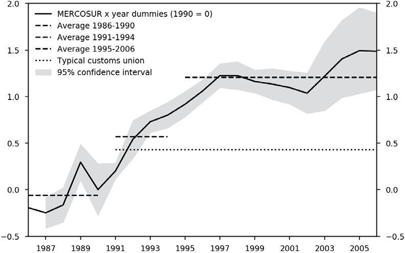
The evidence is consistent with this pattern. We plot estimates of μt in Figure 1. The continuous
line traces out the evolution of point estimates, with the coefficient for the year 1990 normalized
to zero. Coefficients are therefore interpreted as differences with respect to the value in the year
immediately before the start of mercosur.12 The coefficients pick up a rapid intensification
of intra-mercosur trade flows between 1991 and 1994. After 1995, the partial effect of the
mercosur dummies continues to intensify, although at a slower pace.
It is tempting to interpret the solitary jump in 1989 as an anticipatory effect of mercosur. As
with most trade agreements, public announcements preceded the establishment of mercosur.
For example, in 1988, Argentina and Brazil signed an Integration, Cooperation and Development
Treaty, with the explicit goal of establishing a common market, which could be joined by other
Latin American countries, although no clear time horizon was given. It is therefore possible that
trade could have risen in anticipation of mercosur. However, the year 1989 also witnessed other
events that confound the inference. In 1989, both Argentina and Brazil experienced significant
macroeconomic instability, with periods of hyperinflation and strong exchange rate fluctuations,
which are likely to lead to fluctuations in trade flows (or their valuation). If these fluctuations
were larger for the important bilateral trade relationship between Argentina and Brazil than
for trade of these countries with other partners, then individual country-year dummy variables
cannot fully absorb them, and the point estimate of μt for 1989 might be affected by events
unrelated to trade policy.
Figure 1 also shows averages of the estimated coefficients for the periods before mercosur
1986–1990, the transitional period 1991–1994, and the period 1995–2006. The two steps are
substantial: the average in the pre-mercosur period is slightly below the 1990 value, at
-0.063. The other two averages are 0.568 and 1.204. Formal statistical tests reported in Table 6
11
In comparison, Baier et al. (2019b) and El Dahrawy Sánchez-Albornoz and Timini (2020), as do papers that
use the Baier-Bergstrand database, use 1995 as the starting date of mercosur. This will lead to an underestimate
of the effect of mercosur if there is an impact on trade flows already in the period 1991–1994.
12
The coefficients used to construct the figure are taken from specification (3) of Table 6.
BANCO DE ESPAÑA 13 DOCUMENTO DE TRABAJO N.º 2114Figure 1: Intensification of trade between mercosur countries
Notes: The continuous line depicts the estimates of μt with the coefficient for the year 1990 normalized to
zero. The coefficients are taken from specification (3) of Table 6. The 95% interval shown as a shaded area is
constructed from standard errors clustered by exporter, importer and year. The line for a typical customs union
is set at the level of the point estimate for the cu dummy variable in specification (3) of Table 6.
confirm that these average values are statistically different from each other at the 1% level
across all specifications. More importantly, a quick back-on-the-envelope partial equilibrium
calculation using these averages implies that mercosur is associated with a rise in intra-bloc
trade of exp(0.568 − (−0.063)) − 1 = 87.8% during the transitional period, and an additional
exp(1.204 − 0.568) − 1 = 89.1% in the period in which it is a full customs union.13 This increase
in trade is substantially higher than that of a typical customs union (other than mercosur) in
the Baier-Bergstrand eia database, which raises international trade flows between its members
by an estimated exp(0.430) − 1 = 53.7%.
Our results are consistent with prior studies and are located at the higher end of the range
of estimates that are obtained using modern methods. Our average estimate for the period
1995–2006 is very close to the coefficient estimated by Baier et al. (2019b), who use the same
database as we do. They report a point estimate of 1.20. El Dahrawy Sánchez-Albornoz and
Timini (2020) use the wtf database by Feenstra and Romalis (2014)—which does not include
intra-national trade flows—and compute intra-national trade flows as the difference between
gdp and exports, and obtain a lower point estimate, at 0.88. This lower coefficient could be
explained by the fact that their coefficient for mercosur also includes the transitional period
1991–1994.14 Estimates using only international trade flows obtain lower estimates: Baier et al.
(2007) and Kohl (2014) report point estimates of 0.78 and a 0.81, respectively. These graduated
partial equilibrium trade impacts—higher when intra-national flows are included, lower when
13
The increase in trade according to the exact formulas that use all individual coefficients instead of the
averages are very close to these approximations (and close to each other), at 88.7% and 87.1%, respectively.
14
In principle, their use of gdp rather than gross output to compute internal trade could also lead to a lower
estimate: if trade agreements systematically lead to an expansion in higher value added activities, then this
would mechanically introduce a downward bias for the coefficient of interest. However, Campos et al. (2021) find
that the inclusion of the fixed effects that are usual in structural gravity estimations alleviates this problem and
that the effects of trade agreements on trade is estimated to be very similar, regardless of how domestic trade
flows are computed.
BANCO DE ESPAÑA 14 DOCUMENTO DE TRABAJO N.º 2114not—are to be expected, as they have been documented, for example, in a recent study by
Vaillant et al. (2020).
To gauge the impact of mercosur on trade flows over time through the lens of a structural
gravity model, we solve for general equilibrium trade flows as described in section 2.4. We do not
choose a base year and, instead, iterate over all years. For each year we construct counterfactual
trade flows by setting that year’s μt to zero, solving the fixed point problem in (6), and deriving
the implied impact on trade flows using the relationships in (7)–(12). The counterfactual
should be interpreted as trade flows that would have occurred if bilateral trade costs between
mercosur countries had remained at their level of 1986 instead of weakening systematically
relative to those with other partners. The counterfactual also removes all general equilibrium
effects that result from lower trade costs between mercosur members. International trade
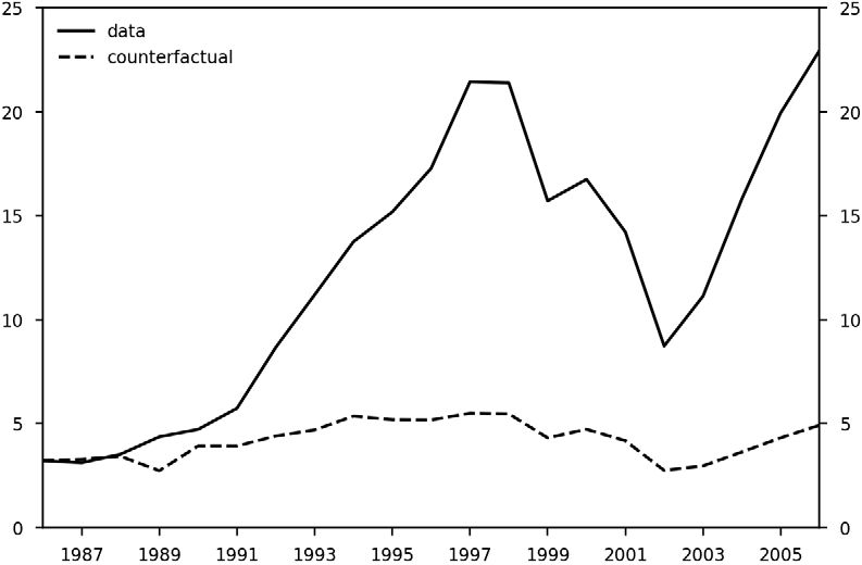
and counterfactual trade between mercosur countries are shown in Figure 2. In this figure
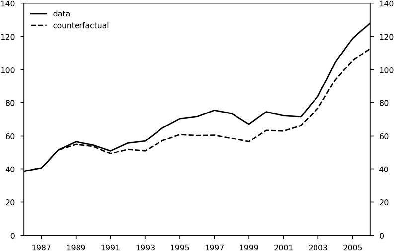
imports equal exports by definition. Figure 3 shows international trade and counterfactual
trade, exports and imports, between mercosur countries and all origins and destinations,
including mercosur.
mercosur appears to have had a substantial impact on trade flows within the trade bloc but a
limited impact on overall trade openness. Figure 2 shows a large and widening gap between
actual data and the counterfactual. From start to end, trade grows by 53% in the counterfactual
scenario while it increased more than 600% in the actual data. The gap widens especially after
1991, coinciding with the start of the initial period of tariff reductions. The 1999 currency crisis
in Brazil and the 2001–2002 crisis in Argentina are clearly visible, both in the actual data and
in the counterfactual; the gap between data and the counterfactual narrows in those years but
starts widening again in 2002. In contrast, Figure 3 shows that the impact of mercosur on
total trade, and therefore trade openness is relatively limited. Before 1991, both lines are hardly
Figure 2: Trade between mercosur countries
Notes: Units are billion constant US dollars for 2010 constructed using consumer inflation for the US (the source
for US inflation is the April 2020 World Economic Outlook database by the IMF. Data and counterfactual are
calculated as the sum of international trade flows between mercosur members (intra-national trade flows are
excluded). The counterfactual is the general equilibrium outcome computed by setting all coefficients μt to zero
and using a trade elasticity of 4.
BANCO DE ESPAÑA 15 DOCUMENTO DE TRABAJO N.º 2114Figure 3: Total exports and imports by mercosur countries
(a) Exports (all international destinations)
(b) Imports (all international origins)
Notes: Units are billion constant US dollars for 2010 constructed using consumer inflation for the US (the source
for US inflation is the April 2020 World Economic Outlook database by the IMF. Total exports is the sum
of all exports by mercosur countries to all destinations, including mercosur as a destination, but excluding
intra-national trade flows. Total imports is the sum of all imports by mercosur countries from all origins,
including mercosur as an origin, but excluding intra-national trade flows. The counterfactual is the general
equilibrium outcome computed by setting all coefficients μt to zero and using a trade elasticity of 4.
distinguishable. In later years, the two lines separate but they remain remarkably close. Part of
the diminished effect on total trade is driven by general equilibrium forces that redirects trade
with other destinations to trade within mercosur. However, the primary reason for the muted
impact on total trade is that trade flows between mercosur members are a small fraction of
total trade, both in actual data and in the counterfactual.
BANCO DE ESPAÑA 16 DOCUMENTO DE TRABAJO N.º 2114The results we have discussed were derived assuming a homogeneous impact of mercosur on
all internal trade relationships. However, it is possible that mercosur had heterogeneous effects
on its members due to their differing economic structures, and also the different configuration
of initial tariffs. Recent research by Baier et al. (2019b) finds evidence of heterogeneous effects
between trade partners in trade agreements in a systematic study using trade flows with the
Yotov et al. (2016) database and, using a different database, El Dahrawy Sánchez-Albornoz
and Timini (2020) find evidence of heterogeneous impacts on trade flows both between and
within Latin American trade agreements, including mercosur.15
We study whether mercosur has a heterogeneous impact on member countries by amending
the baseline specification in (15). A complete disaggregation into directed pair-year effects
within mercosur is infeasible, as it would imply that each coefficient is estimated from a single
observation. It is therefore convenient to group years. Based on the previous analysis, we use
1986–1990, 1991-1994, and 1995-2006 as the three periods of interest. By doing so, we move
away from exploring the year-by-year evolution of the intensification of trade and focus on the
longer terms effects of mercosur. Formally, we allow for variation of the coefficient of interest
along origin country i and destination country j, i.e., by turning the coefficient μt into μijt
leaving the rest of the specification in (15) unchanged. To group the coefficients into periods,
we restrict the coefficients μijt to be constant in across in the period 1991-1994 and in the
period 1995-2006 (the period 1986–1990 is the excluded category). We also consider the case of
heterogeneous but symmetric trade impacts, which corresponds to estimations that restrict the
coefficients to satisfy symmetry, i.e., μijt = μjit . Results are shown in Table 7 in the appendix.
In Tables 1 and 2 we show the implied partial equilibrium impact on trade flows from these
estimations.
In Table 1 we report results for a symmetric specification. There are three stylized facts that
emerge. We find that
1. mercosur has a particularly strong impact on trade links involving Argentina,
2. the link between Argentina and Brazil shows the greatest impact, and
3. trade flows between Paraguay and Uruguay strengthen, especially in the 1995–2006 period.
A specification that lifts the symmetry assumption, and allows for different effects depending on
the direction of trade, allows to refine these findings. Results without the symmetry assumption
are shown in Table 2. All three stylized fact continue to hold. Both exports and imports of
Argentina attributed to mercosur grow substantially. We find that this intensification of
trade is stronger for Argentina’s imports; their growth rates roughly double those of exports.
In addition, we find that exports from Brazil to Argentina attributed to mercosur have
the highest growth rate, exceeding 600%. Moreover, we find that mercosur increased trade
between Paraguay and Uruguay in both directions, with a higher impact on exports from
Paraguay to Uruguay. An additional finding of the heterogeneous specification is that some
directional impacts are small, or even negative.16 As highlighted by Waugh (2010), among
15
As mentioned in the introduction, Baier et al. (2019a) estimate heterogeneous effects of nafta. Esteve-Pérez
et al. (2020) also report heterogeneous effects on bilateral trade flows for countries in the European Monetary
Union.
16
However, only the impact on flows from Paraguay to Brazil in the 1995–2006 period is negative and
significantly different from zero.
BANCO DE ESPAÑA 17 DOCUMENTO DE TRABAJO N.º 2114Table 1: Partial equilibrium trade impact of mercosur assuming
symmetrya,b
from/to Argentina Brazil Paraguay Uruguay
Period 1991–1994
Argentina 155 129 85
Brazil 155 11 -1
Paraguay 129 11 49
Uruguay 85 -1 49
Period 1995–2006
Argentina 451 187 109
Brazil 451 60 1
Paraguay 187 60 229
Uruguay 109 1 229
a
Changes are expressed in percentage points. Exporters in rows, importers
in columns. The coefficients used for the calculations are reported in
Table 7, specification (1).
b
The italic font denotes a calculation based on a coefficient that is sig-
nificantly different from zero at the 5% level. The bold font denotes a
calculation based on a coefficient that is significantly different from zero
at the 1% level.
others, directional pair fixed effects may be better equipped for obtaining unbiased estimates if
trade is unbalanced or trade costs are asymmetric. Baier et al. (2019b) argue that the estimation
of country-specific coefficients increases the likelihood that estimates reflect omitted factors. In
our case, exports from Paraguay to Brazil start out from a very low value in the data, which
may partially explain the large magnitude of this particular negative estimate.
Table 2 shows the partial equilibrium trade impact. To compute the general equilibrium trade
impact we again iterate over all years and compare a scenario with mercosur to a scenario
without mercosur. We convert nominal trade flows in each year to constant US dollars and
then average them over the three periods of interest. Table 3 reports the resulting growth rates
of trade flows attributed to mercosur.
For trade within mercosur, the general equilibrium flows are a muted version of the partial
equilibrium flows, although the stylized facts remain unchanged. Relative to a counterfactual
scenario without mercosur, within-bloc trade increases by 93% in 1991–1994 and 208% in
1995–2006. The impact of mercosur on trade relations with the rest of the world differs by
country: Argentina and Paraguay experience an increase in their exports while those of Brazil
and Uruguay decrease. On the other hand, imports from the rest of the world fall by 8% in the
case of Argentina and by 18% for Paraguay, as they are replaced by within-bloc trade, while
those of Brazil and Uruguay are roughly unchanged.
The degree to which mercosur influences trade openness, and therefore gains from trade, also
differs by country. Argentina experiences the largest opening to international trade, as internal
flows drop by 6%. In Paraguay and Uruguay internal trade flows fall by 5.5% and almost 3%,
whereas for Brazil they decrease but by less than 1%.17
17
Because we constructed data for Paraguay ourselves, it is convenient to check whether these data have an
impact on the results from other countries. In Table 12 in the appendix we replicate the general equilibrium
exercise and find that results are very similar.
BANCO DE ESPAÑA 18 DOCUMENTO DE TRABAJO N.º 2114Table 2: Partial equilibrium trade impact of mercosur without
the symmetry assumptiona,b
from/to Argentina Brazil Paraguay Uruguay
Period 1991–1994
Argentina 123 111 30
Brazil 202 14 -15
Paraguay 323 13 7
Uruguay 181 22 61
Period 1995–2006
Argentina 301 160 71
Brazil 632 85 -7
Paraguay 467 -55 285
Uruguay 132 10 169
a
Changes are expressed in percentage points. Exporters in rows, importers
in columns. The coefficients used for the calculations are reported in
Table 7, specification (3).
b
The italic font denotes a calculation based on a coefficient that is sig-
nificantly different from zero at the 10% level. The bold font denotes a
calculation based on a coefficient that is significantly different from zero
at the 1% level.
The effects on trade—and therefore welfare—are heterogeneous across mercosur members,
not only because the estimated reductions in bilateral trade costs are heterogeneous, but
Table 3: General equilibrium trade impact of mercosura
from/to Argentina Brazil Paraguay Uruguay mercosurb RoWc All destinations
1991-1994
Argentina -2.7 138 107 50 112 4 19
Brazil 173 0.1 4 -9 94 -2 5
Paraguay 305 20 -2.9 22 62 3 21
Uruguay 136 13 37 -0.1 52 -9 12
mercosurb 169 94 24 10 93 -1 8
RoWc -7 2 -6 10 -1 0.0 0.0
All origins 10 7 1 10 8 0.0 0.1
1995-2006
Argentina -6.0 310 113 70 239 1 29
Brazil 541 -0.6 46 -10 250 -2 9
Paraguay 495 -47 -5.5 343 17 17 17
Uruguay 108 9 114 -2.9 31 -2 10
mercosurb 484 202 62 19 208 -2 14
RoWc -8 2 -18 -1 -2 0.0 0.0
All origins 24 10 -2 7 13 0.0 0.1
a
Percent change in trade flows in general equilibrium computed for a trade elasticity of 4. Exporters
are in rows, importers in columns. Intra-national trade flows (the first four elements on the diagonals)
are shown in italics. All other cells exclude intra-national trade. Changes are expressed with respect to
a counterfactual in which trade intensification due to mercosur does not occur and are measured in
percentage points. The coefficients used for the computations are from the specification with heterogeneous
directional trade effects in Table 7, column (3).
b
The definition of mercosur excludes the own country in cells that show a trade flow from/to Argentina,
Brazil, Paraguay, or Uruguay. In all other cells, these four countries are included in the definition.
c
RoW (rest of the world): all countries except the mercosur countries: Argentina, Brazil, Paraguay, and
Uruguay.
BANCO DE ESPAÑA 19 DOCUMENTO DE TRABAJO N.º 2114also because factors that affect the general equilibrium, such as a country’s size, differ across
countries.18 To separate the role payed by the heterogeneity in estimates, in Table 11 (in the
appendix) we compute the general equilibrium impact from assuming that mercosur has a
homogeneous effect on trade costs for member countries. As expected, the general equilibrium
impact on trade flows becomes more similar across countries, i.e., lower in the case of trade
flows involving Argentina and larger for those between other bloc members. In particular, the
computation assuming homogeneity leads to a sizable impact on intra-national trade flows, and
therefore welfare gains, for Uruguay (-11.5% instead of -2.9%) and Paraguay (-9.3% instead of
-5.5%). In other words, disregarding heterogeneity leads to a substantial overestimation of the
effect of mercosur on trade openness and welfare for the two smaller countries. Because the
change in trade openness translates directly into welfare calculations, this difference highlights
the importance for our purposes of allowing for heterogeneity in the coefficients estimated in
the gravity equations.
4 Gains from trade
In the previous section we analyzed the impact of mercosur on trade flows. By participating
in mercosur, all four countries experience a reduction in their domestic trade shares. Using
the change in domestic shares, from (13), gains from trade—in growth rates—are equal to
ΔGi 1/
Gi = λ̂ii − 1. Gains from trade are expressed in terms of consumption of a representative
agent in each country. We conduct various experiments changing the structure of mercosur.19
Results are reported in Table 4. For all calculations, we solve for a counterfactual scenario as
described in Section 2.4 for the three more recent years of data (2004–2006).20 The results in
the table are calculated in averages of trade flows over this period, after expressing trade flows
in constant US dollars.
In a first experiment we simulate a complete disintegration of mercosur. We follow the
standard approach in the literature (e.g., Baier et al. 2019a and Mayer et al. 2019) and simulate
the disintegration by assuming that the effect on trade costs of establishing and dismantling
a trade agreement are symmetric.21 This simulation reveals that a dissolution of mercosur
would reduce gains from trade by 4.0% in Argentina. For the other countries, the welfare loss
induced by a dissolution of mercosur would be smaller; for all three countries, their gains from
trade would be reduced by less than 1%. These results are consistent with the prior finding
that mercosur has had an impact primarily on the trade relationship between Argentina and
the other partners. The central role played by Argentina within mercosur also explains why
in our second scenario (shown in the second panel in the table) a unilateral exit by Argentina
would impact all the other members of the trade bloc so strongly. The other scenarios show that
an exit by Brazil would have a substantial negative impact on welfare in Argentina but a small
18
In structural gravity models, reductions in bilateral trade costs always lead to welfare gains for all countries
involved. However, some countries may gain more than others even if the reduction in trade costs is homogeneous
across countries.
19
These scenarios are not a merely of hypothetical interest. Member countries of mercosur have recurrently
expressed threats of leaving the bloc. See for example Preissler Iglesias and Gamarski (2019).
20
By choosing only the three most recent years we exclude the period 2002–2003, which includes a currency
crisis in Argentina, and may have led to temporary atypical trade flows.
21
Glick and Rose (2016) argue that the symmetry assumption is reasonable for currency unions. For trade
agreements, it assumes that a disintegration implies the reestablishment of both tariffs and non-tariff barriers
that were eliminated with the agreement.
BANCO DE ESPAÑA 20 DOCUMENTO DE TRABAJO N.º 2114Table 4: Gains from trade in mercosura
All origins and destinations With trade bloc Multilateral index Gains
Domestic Exports Imports Exports Imports Inward Outward from trade
1. Trade bloc disintegrates
Argentina 18 -20 -20 -71 -82 -17 -18 -4.0
Brazil 0 -7 -10 -72 -70 2 -1 -0.3
Paraguay 6 -16 2 -18 -38 -15 -2 -0.5
Uruguay 3 -7 -6 -26 -14 -2 -4 -0.8
2. Argentina exits
Argentina 18 -20 -20 -71 -82 -17 -18 -4.0
Brazil 0 -7 -9 -70 -70 2 -1 -0.3
Paraguay 2 -21 -1 -41 -10 -3 -3 -0.5
Uruguay 3 -6 -6 -19 -16 -4 -4 -0.7
3. Brazil exits
Argentina 18 -18 -19 -64 -79 -17 -17 -3.8
Brazil 0 -7 -10 -73 -70 2 -1 -0.3
Paraguay 3 11 4 35 -21 -12 1 0.2
Uruguay -1 1 1 2 3 1 1 0.1
4. Paraguay exits
Argentina 0 0 0 -2 -1 0 0 -0.1
Brazil 0 0 0 -2 1 0 0 0.0
Paraguay 6 -16 2 -19 -38 -16 -2 -0.5
Uruguay 0 0 0 -2 -1 0 0 0.0
5. Uruguay exits
Argentina 0 -1 -1 -4 -2 0 -1 -0.1
Brazil 0 0 0 1 0 0 0 0.0
Paraguay 0 -4 0 -8 -2 0 -1 -0.1
Uruguay 3 -7 -7 -28 -15 -2 -4 -0.8
a
All numbers are expressed in percent deviations from the status quo. The first scenario computes the general
equilibrium impact of a dissolution of mercosur. The other scenarios compute the general equilibrium impact of
a single country leaving the trade bloc. A trade elasticity of 4 is used in all scenarios.
positive impact on Paraguay and Uruguay, who benefit from increased trade with Argentina
once Brazil is removed from the trade bloc. Finally, an exit by either Paraguay or Uruguay,
would reduce the welfare of the country involved, leaving that of the other countries mostly
unchanged.
Across scenarios, Brazil, the largest trade bloc member, is least affected by disruptions of
mercosur. In Brazil, trade with mercosur and also overall international trade is small relative
to intra-national trade, both in the actual data and in the counterfactual scenarios, leading
to small changes in welfare.22 Notably, an exit of Brazil would impose substantial trade costs
on Argentina, its main trade partner within the bloc, but lead to a drop that is an order of
magnitude lower for Brazil. One of the main reasons that explain this findings is the relative
size of Argentina and Brazil’s internal market (with respect to their external sector).
22
The fact that Brazil is relatively closed to international trade has been studied before. Canuto et al. (2015)
explain Brazil’s low import and export penetration by an idiosyncratic economic structure that relies primarily
on domestic value chains instead of global production networks.
BANCO DE ESPAÑA 21 DOCUMENTO DE TRABAJO N.º 2114The low gains from trade derived from trading with mercosur members leads to the question
whether Brazil could gain by switching from mercosur to other preferred trade partners. The
most likely candidates include an integration with other Latin American countries, or even
signing an agreement with nafta, the European Union, or with China. However, agreements
with other trade blocs impose certain costs. They require time for negotiations and spending
political capital; they may influence domestic variables, such as income inequality, imply changes
in regulation, or affect the environment, sometimes with undesired consequences. Additionally,
exiting a consolidated trade agreement may have economic consequences beyond direct trade
effects, by increasing uncertainty, disrupting existing global and regional value chains, etc.
There may also be other payoffs to Brazil from remaining a member of mercosur. Among
them are the democratic clause of mercosur, migration regulations tied to mercosur and,
more generally, the value placed on Latin American integration.
The argument that a country does not always prefer a trade agreement that maximizes gains
from trade can be formally rationalized by modeling the choices of a decision maker whose
objective function includes other considerations besides gains from trade. We define a function
Ri (θ) > 0 that scales gains from trade to denote all other consequences of changing trade policy
to the matrix of trade costs θ and write the value of trade policy θ for the decision-maker in
country i as:
Vi (θ) = Ri (θ)Gi (θ). (16)
Because Gi (θ) is the ratio between total nominal expenditure on final goods in a country and
an ideal price index it can be interpreted as the consumption by a representative agent in each
country. The term Ri (θ) scales up or down consumption of this representative agent, as in the
consumption-based welfare measure of Lucas (2003). The function R(θ) may include concerns
about inequality or the environment, which are not captured in the gains from trade measure,
or the various (economic, political, social, etc.) costs or political economy motivations described
above.23 The factor R(θ) should not be interpreted simply as a parameter but can be thought of
as an endogenous result of a process in which the decision-maker has exhausted all possibilities
of improving the situation after switching to an alternative new trade agreement.24
The decision-maker in a country finds it worthwhile to change trade policy if
ΔVi ΔRi ΔGi
≈ + ≥ 0, (17)
Vi Ri Gi
with indifference if the weak inequality becomes an equality. This implies that a new trade
policy will not be adopted if positive gains from trade are more than compensated by a negative
value of ΔR i
Ri .
To quantify the value placed by Brazil on mercosur, we consider different scenarios in which
Brazil exits mercosur and enters a closer relationship with other trade blocs or countries.
This depends on the type of trade or integration agreement considered, and on the assumed
effect of the agreement on trade flows. We simulate the effects of Brazil signing a customs union
23
Recent examples that use a multiplicative specification as in (16) include the models by Heid and Larch
(2016), where Ri captures changes in employment and Carrère et al. (2015), where it captures aversion to
inequality.
24
Results in this section are derived in the theoretical appendix (Appendix A).
BANCO DE ESPAÑA 22 DOCUMENTO DE TRABAJO N.º 2114with other trade blocs, which implies a relatively strong relationship with its new partners.
Particularly, most scenarios imply the establishment of a customs unions involving countries in
different geographical regions, while customs unions tend to be an intra-regional phenomenon
(Lake and Yildiz, 2016). In this sense, results should be interpreted as upper bounds on the
gains from trade from joining different blocs of countries. We simulate the impact of a customs
union using the coefficient that we estimated for this type of agreement over the whole period
(1986–2006). We interpret this value as the ex-ante estimate of the increase in trade in a
typical customs union. This estimate has the benefit that it would also be available to the
decision-maker at the time of the decision, which we place in the second half of the 2000s.
We report changes in trade flows and the resulting gains from trade in Table 5. Numbers
reported are the net effect of Brazil withdrawing from mercosur and joining a customs union
with different trade blocs or countries. The different alternatives we consider are the group of
countries which would later form Alianza del Pacı́fico (Chile, Colombia, Peru, Mexico), nafta
(Canada, Mexico, the US), and the European Union (the group of countries after the 2004
expansion but before the 2007 expansion).25 We also report results for a customs union with
two individual countries: China and the US.
Table 5: Net impact for Brazil of withdrawing from mercosur and forming a customs
union with another trade bloca
All origins and destinations Multilateral index Gains
Domestic Exports Imports Inward Outward from trade
Alianza del Pacı́fico 0 -3 -5 0 -1 -0.2
nafta -1 8 11 -1 2 0.3
European Union -2 6 9 3 2 0.3
US -1 5 7 0 1 0.2
China 0 -4 -6 3 -1 -0.2
a
All numbers are expressed in percent deviations from the status quo. Scenarios compute the general
equilibrium impact of Brazil withdrawing from mercosur and joining a customs union with a different
trade bloc. A trade elasticity of 4 is used in all scenarios.
The overall conclusion from Table 5 is that net gains from some alternatives are positive,
although they do not exceed 0.3%. The simulations indicate that, although Brazil would become
more open to international trade by leaving mercosur and signing a customs union agreement
with either the European Union or the US, the gains from trade would not be substantial. The
signature of a customs union agreement would probably also impose regulatory changes in
Brazil or lead to other changes that would be costly for the decision-maker. In fact, because
Brazil did not seek to enter an agreement with nafta or the European Union during the
Ri ≤ −0.3 was associated to these
2000s, a revealed preference argument suggests that a value ΔR i
choices.
In conclusion, although Brazil does not exact substantial gains from trade from mercosur, the
incentives to leave mercosur to join another trade bloc are small, and probably overshadowed
by other economic and political economy considerations.
25
An analysis of the recent trade agreement between the European Union and mercosur is outside the scope
of the paper. See Timini and Viani (2020) for an in-depth study of this particular trade agreement.
BANCO DE ESPAÑA 23 DOCUMENTO DE TRABAJO N.º 21145 Conclusion
In this paper we estimate the impact of mercosur on trade flows and on gains from trade for its
member countries. We find that Argentina occupies a central role, with trade flows into and out
of Argentina due to mercosur strengthening more than for the other members of the trade bloc.
Gains from trade are largest for Argentina and smallest for Brazil. Using a general equilibrium
quantitative structural gravity model, we estimate that the dissolution of mercosur would
reduce welfare derived from gains from trade by 4.0% (in consumption-equivalent terms) in
Argentina, and by much smaller amounts, 0.8%, 0.5% and 0.3%, in Uruguay, Paraguay and
Brazil.
Because of the reduced gains from trade that accrue to Brazil, we study whether Brazil would
be better off by withdrawing from mercosur and joining a different trade bloc. Counterfactual
scenarios show that the net gains from trade to Brazil of switching into other existing trade
agreements would be 0.3% of consumption of a representative agent, at most, a small but
positive number. However, as we discuss in the text, it is likely that Brazil’s decision to remain
in mercosur was driven by other (economic, political, social, etc.) considerations.
Our results are subject to a number of well-known caveats. Our methodology does not explicitly
account for dynamics and input-output linkages and our empirical results rely on data on
manufacturing goods alone. Certainly, the inclusion of trade in agricultural products and
services would enrich the analysis. Moreover, the aggregate nature of the manufacturing data
we use does not allow to shed light on interesting phenomena such as the integration in the
automotive industry within mercosur, where trade flows encompass both intermediate and
final goods.
Our results shed light on the more general question of how bilateral trade flows and gains
from trade are distributed among trade bloc members. In the case of mercosur we uncover
a substantial amount of heterogeneity. It would be interesting to see an application of the
techniques of modern quantitative trade models that we use in this paper to other trade blocs,
to detect to what extent mercosur is an example of a more general pattern.
BANCO DE ESPAÑA 24 DOCUMENTO DE TRABAJO N.º 2114You can also read