Masses and compositions of three small planets orbiting the nearby M dwarf L231-32 (TOI-270) and the M dwarf radius valley
←
→
Page content transcription
If your browser does not render page correctly, please read the page content below
MNRAS 507, 2154–2173 (2021)                                                                                              https://doi.org/10.1093/mnras/stab2143
Advance Access publication 2021 August 24

Masses and compositions of three small planets orbiting the nearby M
dwarf L231-32 (TOI-270) and the M dwarf radius valley
V. Van Eylen ,1,2‹ N. Astudillo-Defru ,3 X. Bonfils,4 J. Livingston ,5 T. Hirano,6 R. Luque ,7,8
K. W. F. Lam,9 A. B. Justesen ,10 J. N. Winn,2 D. Gandolfi ,11 G. Nowak ,7,8 E. Palle,7,8 S. Albrecht,10
F. Dai,12 B. Campos Estrada,13 J. E. Owen ,13 D. Foreman-Mackey,14 M. Fridlund ,15,16 J. Korth ,17
S. Mathur,7,8 T. Forveille,4 T. Mikal-Evans ,18 H. L. M. Osborne ,1 C. S. K. Ho ,1 J. M. Almenara ,4
E. Artigau,19 O. Barragán ,20 S. C.C. Barros,21,22 F. Bouchy,23 J. Cabrera,24 D. A. Caldwell,25

                                                                                                                                                                   Downloaded from https://academic.oup.com/mnras/article/507/2/2154/6356971 by guest on 17 September 2021
D. Charbonneau,26 P. Chaturvedi,27 W. D. Cochran,28 S. Csizmadia ,24 M. Damasso,29 X. Delfosse,4
J. R. De Medeiros,30 R. F. Dı́az,31 R. Doyon,19 M. Esposito,27 G. Fűrész,32 P. Figueira,21,33 I. Georgieva,15
E. Goffo,11 S. Grziwa,18 E. Guenther,27 A. P. Hatzes,27 J. M. Jenkins,34 P. Kabath,35 E. Knudstrup ,10
D. W. Latham,26 B. Lavie,23 C. Lovis,23 R. E. Mennickent ,36 S. E. Mullally,37 F. Murgas,7,8
N. Narita,7,38,39,40 F. A. Pepe,23 C. M. Persson,15 S. Redfield ,41 G. R. Ricker,18 N. C. Santos,21,22
S. Seager,18,42,43 L. M. Serrano ,11 A. M. S. Smith,24 A. Suárez Mascareño,8 J. Subjak,34
J. D. Twicken,25,34 S. Udry,23 R. Vanderspek42 and M. R. Zapatero Osorio44
Affiliations are listed at the end of the paper

Accepted 2021 July 21. Received 2021 July 20; in original form 2020 December 10

ABSTRACT
We report on precise Doppler measurements of L231-32 (TOI-270), a nearby M dwarf (d = 22 pc, M = 0.39 M , R =
0.38 R ), which hosts three transiting planets that were recently discovered using data from the Transiting Exoplanet Survey
Satellite (TESS). The three planets are 1.2, 2.4, and 2.1 times the size of Earth and have orbital periods of 3.4, 5.7, and 11.4 d. We
obtained 29 high-resolution optical spectra with the newly commissioned Echelle Spectrograph for Rocky Exoplanet and Stable
Spectroscopic Observations (ESPRESSO) and 58 spectra using the High Accuracy Radial velocity Planet Searcher (HARPS).
From these observations, we find the masses of the planets to be 1.58 ± 0.26, 6.15 ± 0.37, and 4.78 ± 0.43 M⊕ , respectively.
The combination of radius and mass measurements suggests that the innermost planet has a rocky composition similar to that
of Earth, while the outer two planets have lower densities. Thus, the inner planet and the outer planets are on opposite sides
of the ‘radius valley’ – a region in the radius-period diagram with relatively few members – which has been interpreted as a
consequence of atmospheric photoevaporation. We place these findings into the context of other small close-in planets orbiting
M dwarf stars, and use support vector machines to determine the location and slope of the M dwarf (Teff < 4000 K) radius valley
as a function of orbital period. We compare the location of the M dwarf radius valley to the radius valley observed for FGK
stars, and find that its location is a good match to photoevaporation and core-powered mass-loss models. Finally, we show that
planets below the M dwarf radius valley have compositions consistent with stripped rocky cores, whereas most planets above
have a lower density consistent with the presence of a H-He atmosphere.
Key words: planets and satellites: composition – planets and satellites: formation – planets and satellites: fundamental parame-
ters – planets and satellites: individual: L231-32.

                                                                                    on both of these fronts. The Transiting Exoplanet Survey Satellite
1 I N T RO D U C T I O N
                                                                                    (TESS) was launched in 2018 April to conduct an all-sky survey
The small, Earth-sized planets that are being discovered around other               and discover transiting planets around the nearest and brightest stars
stars may or may not resemble our own Earth in terms of composition,                (Ricker et al. 2014). Because the transit signal varies inversely as the
formation history, and atmospheric properties. They are also a                      stellar radius squared, searching small M dwarf stars is of particular
challenge to study, because they produce such small transit and radial-             interest because there is a greater opportunity to find small planets.
velocity (RV) signals. Fortunately, recent progress has been made                   For the same reason, planets around M dwarfs are valuable targets
                                                                                    for atmospheric studies through transmission spectroscopy. To under-
                                                                                    stand which planets have a rocky composition and whether they are
   E-mail: v.vaneylen@ucl.ac.uk

                                                                                                                                         C 2021 The Author(s)

       Published by Oxford University Press on behalf of Royal Astronomical Society. This is an Open Access article distributed under the terms of the Creative
    Commons Attribution License (http://creativecommons.org/licenses/by/4.0/), which permits unrestricted reuse, distribution, and reproduction in any medium,
                                                                                                                   provided the original work is properly cited.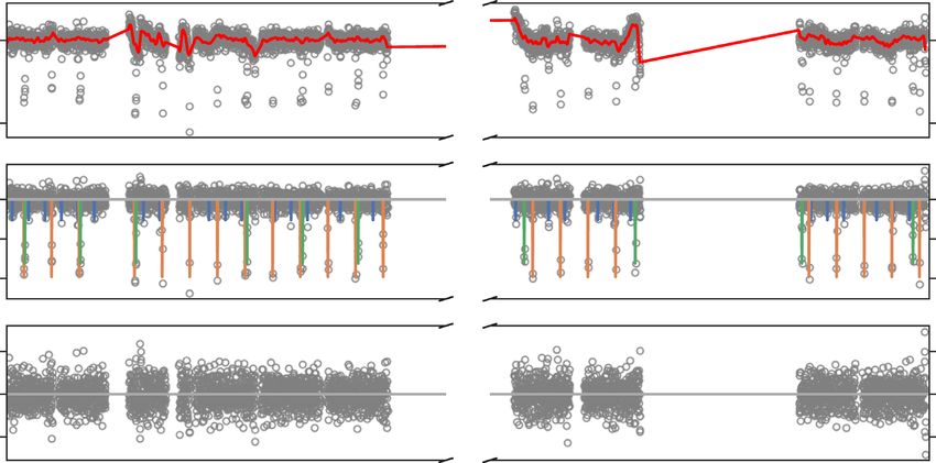
L231-32 and the M dwarf radius valley                             2155
likely to have atmospheres, precise radius measurements from transit       2020 December 16) in the 2-min cadence mode. The data observed
surveys need to be paired with mass measurements from dynamical            in sector 30 were taken on CCD 4 of camera 3, while the data
observations such as precise RV measurements. To this end, the novel       observed in sector 32 were taken on CCD 3 of camera 3. The data
Echelle Spectrograph for Rocky Exoplanet and Stable Spectroscopic          were reduced by the TESS data processing pipeline developed by the
Observations (ESPRESSO, Pepe et al. 2010, 2014, 2020) at the Very          Science Processing Operations Center (SPOC, Jenkins et al. 2016),
Large Telescope (VLT) provides an unprecedented RV precision.              and the transits of three planet candidates were detected in the SPOC
   Here, we present the result of an ESPRESSO campaign (ESO                pipeline and promoted to TESS object of interest (TOI) status by the
observing program 0102.C-0456) to characterize three small (1.1,           TESS science team.
2.3, and 2.0 R⊕ ) transiting planets around L231-32 (TOI-270), a              We started radial velocity (RV) observations to confirm and
nearby (22 pc), bright (K = 8.25, V = 12.6), M3V dwarf star (M =          measure the mass of these transiting planets with ESPRESSO and
0.39 M , R = 0.38 R ), as well as four additional ESPRESSO              with HARPS, on 2019 February 9 and 2019 January 1, respectively
observations obtained as part of observing programs 1102.C-0744            (see Section 2.2). As these observations were ongoing, Günther et al.
and 1102.C-0958. We also used data from the High Accuracy Radial           (2019) also reported on the validation of these planets, by performing

                                                                                                                                                            Downloaded from https://academic.oup.com/mnras/article/507/2/2154/6356971 by guest on 17 September 2021
velocity Planet Searcher (HARPS) program for M-dwarf planets               a statistical analysis of the TESS observations, as well as obtaining
amenable to detailed atmospheric characterization (ESO observing           ground-based seeing-limited photometry coordinated through the
program 1102.C-0339). These planets were observed to transit by            TESS Follow-up Observing Program (TFOP).1
TESS in three subsequent campaigns, each lasting about 27 d. The              We downloaded the TESS photometry from the Mikulski Archive
transit signals were described and validated by Günther et al. (2019).    for Space Telescopes (MAST2 ) and started our analysis using the
Because of the characteristics of the host star and its planets, L231-32   presearch data conditioning (PDC) light curve reduced by SPOC.
is a prime target for exoplanet atmosphere studies, which are ongoing      We searched for additional transit signals using a Box Least-Square
with the Hubble Space Telescope (HST, program id GO-15814, PI              (BLS) algorithm (Kovács, Zucker & Mazeh 2002) and the ‘Détection
Mikal-Evans; Mikal-Evans et al. 2019). Furthermore, simulations            Spécialisée de Transits’ (DST) algorithm (Cabrera et al. 2012) for
have shown these planets are highly suitable for atmospheric char-         additional transit signals but found no evidence for any transiting
acterization with the James Webb Space Telescope (JWST; Chouqar            planets in addition to the three that were alerted. In Section 4.1, we
et al. 2020). Further transit observations with e.g. TESS or other         describe our approach to the modelling of the TESS photometry.
space telescopes may reveal transit timing variations (TTVs) which
can be used to constrain the planet masses independently of RVs.           2.2 Spectroscopic observations
   Our mass measurements for these three planets allow us to
constrain their possible compositions. The planets are located on          2.2.1 ESPRESSO
both sides of the radius valley, which separates close-in super-Earth      We obtained 26 high-resolution spectroscopic observations of L231-
planets from sub-Neptune planets (e.g. Lopez & Fortney 2013; Owen          32 between 2019 February 9 and 2019 March 22 using ESPRESSO
& Wu 2013; Fulton et al. 2017; Van Eylen et al. 2018), and we              (Pepe et al. 2014, 2020) on the 8.2 m Very Large Telescope (VLT;
show how their compositions can be interpreted in this context. We         Paranal, Chile) as part of observing program 0102.C-0456. Four
furthermore compare the properties of L231-32’s planets with those         additional observations were obtained as part of observing programs
of other small planets with precisely measured masses, radii, and          1102.C-0744 and 1102.C-0958. ESPRESSO is a relatively novel
periods, and use this sample to measure the location of the M dwarf        instrument at the VLT which was first offered to the community in
radius valley and its slope as a function of orbital period.               2018 October.
   This paper is organized as follows. In Section 2, we describe              Each observation has an integration time of 1200 s, a median
the TESS transit observations, and ESPRESSO and HARPS RV                   resolving power of 140 000, and a wavelength range of 380–788 nm.
observations. In Section 3, we derive the parameters of the host star,     We used the slow read-out mode, which uses a 2 × 1 spatial by
by combining high-resolution spectra with other sources of ancillary       spectral binning. Observations were taken in high-resolution (HR)
information. In Section 4, we describe the approach to modelling           mode. One of the observations was flagged as unreliable due to a
L231-32 and the properties of its planets. In Section 5, we show the       detector restart just before the exposure, and we excluded this data
resulting properties of L231-32’s planets and discuss the composition      point from the analysis as a restart can result in additional noise.
of the planets. In Section 6, we compare their properties to radius        This leaves a total of 29 ESPRESSO observations that we use in our
valley predictions and to other planets orbiting M dwarf stars, and        subsequent analysis.
measure the location and slope of the M dwarf radius valley. Finally,         To determine a wavelength-calibration solution, daytime ThAr
in Section 7, we provide a brief summary and conclusions.                  measurements were taken and the source was observed with simulta-
                                                                           neous Fabry–Pérot (FP) exposures, following the procedure outlined
                                                                           in the ESPRESSO user manual.3 The signal-to-noise ratio (SNR) for
2 O B S E RVAT I O N S A N D M O D E L L I N G                             individual spectra at orders 104 and 105, which are both centred at
                                                                           557 nm, ranges from 9 to 40, with a median SNR of 29.
2.1 TESS photometry                                                           To calibrate and reduce the data we used the publicly available
L231-32 (TOI-270; TIC 259377017) was observed by the TESS                  pipeline for ESPRESSO data reduction,4 together with the ESO
mission (Ricker et al. 2014) during three 27-d sectors, namely sectors     Reflex tool (Freudling et al. 2013). This tool uses the science
3, 4, and 5, between 2018 September 20 and 2018 December 11. It
was observed on CCD 4 of camera 3 in sector 3 and 4, and on                1 https://tess.mit.edu/followup/
CCD 3 of camera 3 in sector 5. The star was pre-selected (Stassun          2 https://archive.stsci.edu/tess
et al. 2018) and was observed in a 2-min cadence for the whole             3 https://www.eso.org/sci/facilities/paranal/instruments/espresso/ESPRES
duration of these sectors. During the TESS extended mission, the           SO User Manual P102.pdf
target was reobserved in sectors 30 (between 2020 September 23             4 http://eso.org/sci/software/pipelines/espresso/espresso-pipe-recipes.html, v

and 2020 October 19) and 32 (between 2020 November 20 and                  ersion 2.0

                                                                                                                  MNRAS 507, 2154–2173 (2021)
2156 V. Van Eylen et al.
spectra and all associated calibration files (i.e. bias frames, dark [Fe/H]sm = −0.20 ± 0.12. To obtain precise stellar parameters, we
frames, led frames, order definitions, flat frames, FP wavelength combined the spectroscopic information with a distance measure-
calibration frame, Thorium-FP calibration, FP-Thorium calibration, ment of the star based on the Gaia parallax (44.457 ± 0.027 mas,
fibre-to-fibre efficiency exposure, and a spectrophotometric standard Gaia Collaboration 2018) and the apparent magnitude of the star
star exposure) to reduce and calibrate the raw spectra, and provide from the 2MASS catalogue (mKs ,2MASS = 8.251 ± 0.029, Skrutskie
one-dimensional and two-dimensional reduced spectra.5 All required et al. 2006). For the Gaia observations, we include an additional
calibration frames are automatically associated with the raw science uncertainty as reported by Stassun et al. (2018), who find a systematic
frames and were simultaneously downloaded from the ESO archive.6 error of 0.082 ± 0.033 mas. We adopted a conservative systematic
We followed the standard pipeline routines for the ESPRESSO data error of 0.115 mas and add this in quadrature to the internal error
reduction pipeline using ESO Reflex. The radial velocities were on the parallax measurement of L231-32. This results in a distance
computed following the procedure described in Astudillo-Defru et al. estimate of dGaia = 22.453 ± 0.060 pc.
(2017b). A slight adaptation to ESPRESSO data was introduced to To determine stellar parameters that combine the information from
construct the stellar template by combining the two Echelle orders the apparent magnitude, distance, and spectra, we implemented a
Downloaded from https://academic.oup.com/mnras/article/507/2/2154/6356971 by guest on 17 September 2021
covering a common spectral range. The template is then Doppler Markov Chain Monte Carlo (MCMC) code to estimate the final
shifted and we maximized its likelihood with each two-dimensional stellar parameters. For this, we defined the log likelihood (log L) as a
reduced spectrum. The mean RV precision is 0.47 m s−1 . The function of the stellar radius (R ) and apparent magnitude (mKs ) as
resulting RV observations are listed in Table A1.
(R − R,sm )2 (mKs − mKs,2MASS )2
2.2.2 HARPS log L ∝ 2
+ . (1)
σR,sm σm2 K
s,2MASS
We used HARPS (Mayor et al. 2003) on the the La Silla 3.6m
telescope to gather 58 additional spectra (program id. 1102.C-0339). The parameters R and mKs are related to each other through the
These high-resolution spectra, with a resolving power of 115 000, empirical relations determined by Mann et al. (2015). These relations
were obtained between 2019 January 1 and 2019 April 17, spanning show how R depends on [Fe/H] and the absolute magnitude MKs ,
89 d. We fixed the exposure time to 1800 s, resulting in a total which in turn is related to the apparent magnitude and the distance
equivalent to 29 h of open shutter time. The read-out speed was set through mKs − MKs = 5 log d − 5. We imposed Gaussian priors on
to 104 kHz. To prevent possible contamination from the calibration [Fe/H] and d, i.e.
lamp in the bluer zone of the spectral range, we elected to put the
calibration fibre on the sky.
Raw data were reduced with the dedicated HARPS Data Reduction ([Fe/H] − [Fe/H]sm )2 (d − dGaia )2
pprior ∝ exp − 2
− . (2)
Software (Lovis & Pepe 2007). The resulting spectra have an SNR 2σ[Fe/H] sm
2σd2Gaia
ranging between 14 and 29 at 550 nm, with a median of 22.
We then extracted RVs, again following Astudillo-Defru et al. For mKs and R , we used a uniform prior distribution. We
(2017b), resulting in an RV extraction consistent with how RVs then sampled the likelihood and prior from equations (1) and (2)
were extracted for ESPRESSO (see Section 2.2.1). The mean RV using a customized MCMC implementation (Hirano et al. 2016),
precision of the HARPS observations is 2.05 m s−1 and the data which employs the Metropolis–Hastings algorithm and automatically
have a dispersion of 5.10 m s−1 . The resulting RVs and stellar optimizes the chain step sizes of the proposal Gaussian samples so
activity indices are listed in Table A2. The mean RV precision of the that the total acceptance ratio becomes 20−30 per cent after running
HARPS observations is 2.17 m s−1 . The HARPS timestamps were ∼106 steps. From the MCMC posterior sample we determined the
converted to Barycentric Dynamical Time (BJDTDB ) for consistency median and 15.87 and 84.13 percentiles to report best values and their
with ESPRESSO and TESS observations. The resulting RVs and uncertainties, which are shown in Table 1. We further determined the
stellar activity indices are listed in Table A2. stellar mass (M ) from its corresponding empirical relation based
on mKs (Mann et al. 2015, equation 5). For both stellar radius and
3 S T E L L A R PA R A M E T E R S stellar mass, we take into account the uncertainty of the empirical
relationships, which are 2.7 per cent and 1.8 per cent, respectively
3.1 Fundamental stellar parameters (Mann et al. 2015). Since the effective temperature (Teff ) does not
affect the empirical relations, we adopt the spectroscopic effective
We co-added the ESPRESSO spectra and analysed the combined
temperature as our final value (Teff = Teff,sm ). We use Teff and R
spectrum of L231-32 to estimate its spectroscopic parameters. We
to determine the stellar luminosity (L), and finally, from mass and
used SPECMATCH-EMP (Yee, Petigura & von Braun 2017), which is
radius we also calculated the stellar density (ρ ) and surface gravity
known to provide accurate estimates for late-type stars. Following
(log g). Interstellar extinction was neglected, as the star is relatively
the prescriptions described in Hirano et al. (2018), we lowered
nearby. All these values are reported in Table 1.
the spectral resolution of the combined ESPRESSO spectrum from
These values can be compared with the stellar parameters derived
140 000 to 60 000 and stored the spectrum in the same format as
by Günther et al. (2019). For example, the stellar mass and radius
Keck/HIRES spectra before inputting it into SPECMATCH-EMP.
determined here, 0.386 ± 0.008 M and 0.378 ± 0.011 R , are con-
Using SPECMATCH-EMP, we determined the stellar effective tem-
sistent with the mass and radius determined by Günther et al. (2019),
perature (Teff,sm ), stellar radius (R,sm ), and metallicity ([Fe/H]sm ),
i.e. 0.40 ± 0.02 M and 0.38 ± 0.02 R , respectively. The values
and found Teff,sm = 3506 ± 70 K, R,sm = 0.410 ± 0.041 R , and
determined here make use of a high-resolution combined ESPRESSO
spectrum in addition to distance and magnitude information and are
5 See the ESPRESSO pipeline user manual for details, ftp://ftp.eso.org/pub/ slightly more precise. Similarly, the temperature determined here,
dfs/pipelines/instruments/espresso/espdr-pipeline-manual-1.2.3.pdf i.e. 3506 ± 70 K, is consistent with the value determined by Günther
6 http://archive.eso.org/ et al. (2019), i.e. 3386+137
−131 K, and more precise.
MNRAS 507, 2154–2173 (2021)L231-32 and the M dwarf radius valley 2157
Table 1. System parameters of L231-32.
Basic properties
TESS ID TOI-270, TIC 259377017, L231-32
2MASS ID J04333970–5157222
Right ascension (hms) 04 33 39.72
Declination (deg) −51 57 22.44
Magnitude (V) V: 12.62. 2MASS, J: 9.099 ± 0.032, H:
8.531 ± 0.073, K: 8.251 ± 0.029, TESS: 10.42, Gaia,
G: 11.63, bp : 12.87, rp : 10.54
Adopted stellar parameters
Effective temperature, Teff (K) 3506 ± 70
Stellar luminosity, L(L ) 0.0194 ± 0.0019
Downloaded from https://academic.oup.com/mnras/article/507/2/2154/6356971 by guest on 17 September 2021
Surface gravity, log g (cgs) 4.872 ± 0.026
Metallicity, [Fe/H] −0.20 ± 0.12
Stellar mass, M (M ) 0.386 ± 0.008
Stellar radius, R (R ) 0.378 ± 0.011
Stellar density, ρ (g cm−3 ) 7.20 ± 0.63
Distance (pc) 22.453 ± 0.059
Parameters from RV and transit fit L231-32b L231-32c L231-32d
Orbital period, P (d) 3.3601538 ± 0.0000048 5.6605731 ± 0.0000031 11.379573 ± 0.000013
Time of conjunction, tc (BJDTDB − 2458385) 2.09505 ± 0.00074 4.50285 ± 0.00029 4.68186 ± 0.00059
Planetary mass, Mp (M⊕ ) 1.58 ± 0.26 6.15 ± 0.37 4.78 ± 0.43
Planetary radius, Rp (R⊕ ) 1.206 ± 0.039 2.355 ± 0.064 2.133 ± 0.058
Planetary density, ρ p (g cm−3 ) 4.97 ± 0.94 2.60 ± 0.26 2.72 ± 0.33
Semimajor axis, a (au) 0.03197 ± 0.00022 0.04526 ± 0.00031 0.07210 ± 0.00050
Equilibrium temperature, Ab = 0, Teq (K) 581 ± 14 488 ± 12 387 ± 10
Equilibrium temperature, Ab = 0.3, Teq (K) 532 ± 13 447 ± 11 354 ± 8
Orbital eccentricity, e 0.034 ± 0.025 0.027 ± 0.021 0.032 ± 0.023
Argument of pericentre, ω (rad) 0 ± 1.8 0.2 ± 1.6 −0.1 ± 1.6
Stellar RV amplitude, K (m s−1 ) 1.27 ± 0.21 4.16 ± 0.24 2.56 ± 0.23
Fractional planetary radius, Rp /R 0.02920 ± 0.00069 0.05701 ± 0.00071 0.05163 ± 0.00069
Impact parameter, b 0.19 ± 0.12 0.28 ± 0.11 0.19 ± 0.11
Inclination, i 89.39 ± 0.37 89.36 ± 0.24 89.73 ± 0.16
Limb darkening parameter, q1 0.17 ± 0.10 0.17 ± 0.10 0.17 ± 0.10
Limb darkening parameter, q2 0.71 ± 0.16 0.71 ± 0.16 0.71 ± 0.16
Noise parameters and hyperparameters from RV and transit fit
Photometric ‘jitter’, σ phot (ppt) 0.5224 ± 0.0049
ESPRESSO RV ‘jitter’, σ 2,rv (m s−1 ) 0.68 ± 0.26
HARPS RV ‘jitter’, σ 2,rv (m s−1 ) 0.16 ± 0.23
GP power (phot), S0 (ppt2 d/2π ) 1.29 ± 0.27
GP frequency (phot), α 0 (2π /d) 1.10 ± 0.11
GP power (RV), S1 (m2 s−2 d/2π ) 22 ± 70
GP frequency (RV), α 1 (2π /d) 0.22 ± 0.36
GP quality factor Q (RV) 3.7 ± 7.3
ESPRESSO offset, γ 0 (m s−1 ) 26850.80 ± 0.56
HARPS offset, γ 0 (m s−1 ) 26814.28 ± 0.36
3.2 Stellar rotation 57.5 ± 5.7 d. We also searched the TESS light curve for rotational
modulation. The PDC pipeline (Smith et al. 2012; Stumpe et al.
We also investigated the activity indicators from the spectra (see
2012, 2014) produces high-quality light curves well suited for transit
Section 2.2) to estimate the stellar rotation period. In doing so,
searches. However, stellar rotation signals can be removed by the
we focused on the HARPS observations, which span a longer
PDC photometry pipeline, so we used the lightkurve package
baseline than the ESPRESSO observations and which are therefore
(Barentsen et al. 2019) to produce systematics-corrected light curves
more suitable to determine the stellar rotation period. We computed
with intact stellar variability. lightkurve implements pixel-level
the Generalized Lomb–Scargle periodogram (GLS; Zechmeister &
decorrelation (PLD; Deming et al. 2015) to account for systematic
Kürster 2009) of both Hα and Na D and found consistent periods
noise induced by intra-pixel detector gain variations and pointing
of P = 54.0 ± 2.4 d and P = 61.5 ± 4.0 d, respectively. We
jitter. We normalized and concatenated the PLD-corrected light
finally also looked at the full width at half-maximum (FWHM) of the
curves, then computed a GLS periodogram of the full time series.
cross-correlation function (CCF), which was extracted for HARPS
A sine-like signal is clearly visible, and GLS detects a significant
observations directly by the Data Reduction Software,7 and find P =
∼1.1 ppt signal at 57.90 ± 0.23 d. We also analysed the full time
series with a pipeline that combines three different methods (a time-
7 http://www.eso.org/sci/facilities/lasilla/instruments/harps/doc/DRS.pdf period analysis based on wavelets, autocorrelation function, and
MNRAS 507, 2154–2173 (2021)2158 V. Van Eylen et al.
composite spectrum) and that has been applied to tens of thousand with multiple transiting planets is low but not necessarily zero (Van
of stars (e.g. Garcı́a et al. 2014; Ceillier et al. 2017; Mathur et al. Eylen & Albrecht 2015; Xie et al. 2016; Van Eylen et al. 2019).
2019; Santos et al. 2019). The time-period and composite spectrum We therefore do not fix eccentricity to zero, but place a prior on
analyses find a signal around 46–49 d. The autocorrelation function the orbital eccentricity, of a Beta distribution with α = 1.52 and
does not converge due to the too short length of the observations, β = 29 (Van Eylen et al. 2019). We sample ω uniformly between
not allowing us to confirm the rotation period with this pipeline. −π and π . We adopt a quadratic limb darkening model with two
Given the length of the data, it can still be possible that we measure parameters, which we reparametrize following Kipping (2013) to
a harmonic of the real rotation period. Since the total time series facilitate efficient uninformative sampling.
only spans 3 × 27 d, it is difficult to ascertain the veracity of this
signal, but it appears consistent with the values determined from
the RV activity indicators. For completeness, we also searched for 4.1.2 Gaussian process noise model
signals in the sector-combined PDC light curve, but detected only
To model correlated noise in the TESS light curve we adopt a
short-time-scale variability.
Downloaded from https://academic.oup.com/mnras/article/507/2/2154/6356971 by guest on 17 September 2021
Gaussian process model (Rasmussen & Williams 2006; Foreman-
We explored the possibility of estimating the stellar rotation period
Mackey et al. 2017). We adopt a stochastically driven damped
from its relationship with the RH K (e.g. Astudillo-Defru et al. 2017a).
harmonic oscillator (SHO) for which the power spectral density is
However, near the Ca II H&K lines, the HARPS data set has an
defined as
extremely low-flux (with a median SNR of about 0.6) that limits the
precision of this approach to measure the stellar rotation rate. We 2 S0 α04
S(α) = , (3)
find log(RH K ) = −5.480 ± 0.238, and estimate a rotation period of π α 2 − α02 2 + 2α02 α 2 /Q20
88 ± 32 d from this approach.
Based on the combination of RV stellar activity indicators, and where α 0 is the frequency of the undamped oscillator and S0 is
the TESS photometry, it appears likely that the stellar rotation period proportional to the power at α = α 0 . The SHO kernel is similar to the
is approximately 58 d, which is consistent with typically observed quasi-periodic kernel, which has been used extensively to model stel-
rotation periods for M dwarf stars in this mass range, i.e. ≈20–60 d lar activity (e.g. Haywood et al. 2014; Grunblatt, Howard & Haywood
(Newton et al. 2016). 2015; Rajpaul et al. 2015), but can be computed significantly faster
and therefore facilitates a joint-fit of the transit observations as well as
both HARPS and ESPRESSO RV data. Since we do not a priori know
4 O R B I TA L A N D P L A N E TA RY PA R A M E T E R S
the values of S0 and α 0 we adopt a broad prior and relatively arbitrary
We modelled the TESS light curve and ESPRESSO RV data using the starting value, in the form of a normal distribution, N (μ, σ ) where
publicly available EXOPLANET code (Foreman-Mackey, Barentsen & μ and σ are the mean and standard deviation of the distribution. We
Barclay 2019). This tool can model both transit and RV observations adopt log α0 ∼ N (log(2π/10), 10) and log S0 ∼ N (log(σphot 2
), 10),
using a Hamiltonian Monte Carlo (HMC) scheme implemented in 2
where σphot is the variance of the TESS photometry. To limit the
Python in PYMC3 (Salvatier, Wiecki & Fonnesbeck 2016), and has number of free parameters, we set Q0 = 1.
been used to model photometric and spectroscopic observations of Furthermore, we add a mean flux parameter (μnorm ) to our model.
other exoplanets (e.g. Kanodia et al. 2020; Plavchan et al. 2020; Since we normalized the light curve to zero, we place a broad prior
Stefansson et al. 2020). Next, we describe the ingredients of our of μnorm ∼ N (0, 10). Finally, we include a noise term, which we
model and the procedure for optimizing and sampling the orbital fit as part of the Gaussian process model. We initalize this term
planetary parameters. based on the variance of the TESS photometry, with a wide prior. All
parameters and priors are summarized in Table A3.
4.1 Light curve model
4.2 Radial velocity model
4.1.1 Transit model
4.2.1 Planet orbital model
We used EXOPLANET to model the TESS transit light curve, which
makes use of STARRY (Luger et al. 2019; Agol, Luger & Foreman- We model the radial velocity (RV) variations of the host star using a
Mackey 2020) to calculate planetary transits. STARRY implements Keplerian model for each planet, as implemented in EXOPLANET. For
numerically stable analytic planet transit models with polynomial each planet, we model the planet mass (Mi ) which is associated with
limb darkening – a generalization of Mandel & Agol (2002) – along an RV semi-amplitude (Ki ). The other parameters that determine the
with their gradients. The transit model contains seven parameters planet orbit (Pi , T0,i , ei , and ωi ) were already defined in Section 4.1.
for each planet (i ∈ {b, c, d}), i.e. the orbital period (Pi ) and transit For Mi we adopt broad Gaussian priors centred on initial guesses of
reference time (T0,i ), the planet-to-star ratio of radii (Rp,i /R ), the the planet mass, based on the observed amplitude of the RV curve.
scaled orbital distance (ai /R ), the impact parameter (bi ), and the Although some RV observations were taken during transit, we
eccentricity (ei ) and argument of periastron (ωi ); furthermore, there did not model the Rossiter–McLaughlin (RM) effect (McLaughlin
are two stellar limb darkening parameters (q1 and q2 ) which are 1924; Rossiter 1924), as its RV amplitude is small relative to our
joint for all three planets. We use a uniform prior for Pi and T0,i RV precision.8
centred on an initial fit of the planet signals, with a broad width of
0.01 and 0.05 d, respectively, which encompasses the final values.
We sample the ratio of radii uniformly in logarithmic space. For bi 8 Based on the estimated rotation period of 58 d (see Section 3.2) and the
we sample uniformly between 0 and 1. We do not directly input stellar radius, we find a stellar rotation speed, i.e. maximum v sin i for i =
a prior distribution for ai /R , because this parameter is directly 90◦ , of 330 m s−1 . Given transit depths of the planets, impact parameters,
constrained by ρ and the other transit parameters. Instead, we and stellar limb darkening we estimate the maximum RM RV amplitude
input M and R to the model using a normal distribution with mean (assuming the planet’s orbit is aligned with the rotation of the star), to be
and sigma as determined in Section 3. The eccentricity of systems ≈0.5 m s−1 (Albrecht et al. 2011).
MNRAS 507, 2154–2173 (2021)L231-32 and the M dwarf radius valley 2159
4.2.2 Noise model RV fit. Comparing the best-fitting masses using both kernels, we find
that they are consistent with a fraction of σ .
In addition to the formal uncertainty on each RV observation (σ rv ,
In summary, these different model choices all result in very similar
see Section 2.2 and Table A1), we define an additional ‘jitter’ noise
mass estimates, and the use of the kernel adopted here results
term (σ 2,rv ) which is added in quadrature. We model this with a wide
in virtually the same results as using a quasi-periodic kernel. We
Gaussian prior as log σ2,rv ∼ N (log(1), 5).
therefore adopt the GP model with the SHO kernel described in
We furthermore model the noise using a Gaussian process model,
Section 4.2.2, as this can be calculated efficiently allowing for a
to model any correlation between the RV observations in a flexible
joint fit with the transit data, and as a GP model can flexibly model
way. This approach has been shown to reliably model stellar
the suspected stellar rotation signal in a reliable way (e.g. Haywood
variability (e.g. Haywood et al. 2014). To do so, we again adopt
et al. 2014). The resulting RV model is shown in Fig. 1. We further
the SHO kernel that was described in Section 4.1.2. As the TESS
calculated the root-mean square (RMS) of the residuals to the best
light curve is modified and filtered, we do not necessarily expect
fit. We find 1.86 m s−1 for HARPS, and 0.95 m s−1 for ESPRESSO.
the photometric noise to occur in a similar way as noise in the RV
These small values confirm the quality of the fit and showcase the
Downloaded from https://academic.oup.com/mnras/article/507/2/2154/6356971 by guest on 17 September 2021
observations, and so the two GP models are kept independent.
precision the ESPRESSO instrument is capable of.
The SHO kernel is defined as in equation (3), where we now have
three hyperparameters S1 , α 1 , and Q1 . In all cases, we adopt broad
priors. The hyperparameter α 1 can be thought of as a periodic term.
4.3 Joint analysis model
We therefore initialize it based on the expected stellar rotation, which
we expect to be at around 55 d (see Section 4.2.3). The list of priors We now combine the transit model and the RV model to run a joint fit
is shown in Table A3. of the TESS and ESPRESSO/HARPS observations. To summarize,
this model contains eight physical parameters for each planet, as
defined in Sections 4.1.1 and 4.2.1, i.e. Pi , T0,i , Rpi /R , ai /R , bi ,
4.2.3 Comparing different RV models ei , ωi , and Mi . In addition, we provide M and R to the model
(see Section 4.1), because these values inform ai /R , and because
As outlined in Section 4.2.2, we adopt a Gaussian process model to the values are used to calculate derived parameters. A mean flux
reliably estimate the planet masses from the RV observations, where parameter, μnorm , is included, as well as a GP model for the transit
the GP component is used to model the stellar rotation and activity light curve as a function of time, as well as a GP model for the
in a flexible manner. We assessed whether this model is suitable for RV data. The resulting parameters are S0 , α 0 , S1 , α 1 , Q1 , σ phot ,
these observations. σ 2,rv,ESPRESSO , and σ 2,rv,HARPS , as defined in Sections 4.1.2 and 4.2.2.
We compared several possible RV models. In the first one, the RVs A summary of all parameters and their priors is given in Table A3. We
are modelled without taking into account any component describing infer the optimal solution and its uncertainty using PYMC3 as built
stellar rotation (i.e. a ‘pure’ 3-planet model, without GP). This into EXOPLANET. PYMC3 uses a Hamiltonian Monte Carlo scheme
model appears to perform significantly worse at modelling the RV to provide a fast inference (Salvatier et al. 2016). As we found the
observations than the models with a GP. Notably, it results in a fit for parameter distribution to be symmetric, we report the mean and
which the residuals have a distinctly correlated structure, and the jitter standard deviation for all parameters in Table 1.
terms are significantly higher, suggesting a component is missing We find that the masses of L231-32b, c, and d are 1.58 ± 0.26 M⊕ ,
from the fit. This is not surprising, as we know the stellar rotation 6.15 ± 0.37 M⊕ , and 4.78 ± 0.43 M⊕ , respectively. In Fig. 2, we
period of about 57 d (see Section 3.2) is likely to influence the RV show the TESS photometry together with the best-fitting transit and
signal. Even so, the resulting best-fitting masses are fully consistent GP models. We show a zoom-in on the transits folded by orbital
with the GP approach to better than 1σ , providing confidence in our period and the RV curve for each planet in Fig. 3.
fitting approach and suggesting that L231-32 is a remarkably quiet
M star.
We also explored models in which we replaced the GP component 5 THE COMPOSITION OF L231-32B, C, AND D
with a polynomial trend instead, where we explored several different
orders. In particular, a third-order polynomial results in a fit where 5.1 Bulk densities and compositions
the polynomial resembles a sinusoid with a ‘peak to peak’ period
of around 50 d, visually similar to the GP model, suggesting it may Combining the mass measurements (see Section 4.3) with the
similarly capture a quasi-periodic stellar rotation. Once again the modelled radii (1.206 ± 0.039 R⊕ , 2.355 ± 0.064 R⊕ , and
planet masses are remarkably consistent, to better than 1σ for all 2.133 ± 0.058 R⊕ ), we find planet densities of 4.97 ± 0.94,
three planets. Another model, in which we included a fourth ‘planet’ 2.60 ± 0.26, and 2.72 ± 0.33 g cm−3 , respectively. This implies
(without polynomial trend), once again provides fully consistent that the density of the smaller inner planet is significantly higher
masses; the orbital period of this ‘planet’ was ∼63 d, consistent than that of the two larger, outer planets.
with the stellar rotation period found in Section 3.2. We furthermore We now place the mass and radius measurements of the planets
explored the specific choice of a GP kernel. For this, we used orbiting L231-32 into context and compare them to composition
RADVEL9 (Fulton et al. 2018). With RADVEL, we modelled the RV models. In Fig. 4, we show a mass-radius diagram for small planets
data using a quasi-periodic kernel, which is similar to the SHO kernel (R < 3 R⊕ and M < 10 M⊕ ). The properties of L231-32 are shown,
described in Section 4.2.2, but the SHO kernel has properties that along with those of other planets for which planet masses and radii
make it significantly faster to calculate (see Section 4.2.2). This are determined to better than 20 per cent. To do so, we made use of the
makes the SHO kernel more suitable for performing a joint transit- TEPcat10 data base (Southworth 2011) as a reference, which includes
9 https://github.com/California-Planet-Search/radvel 10 https://www.astro.keele.ac.uk/jkt/tepcat/
MNRAS 507, 2154–2173 (2021)2160 V. Van Eylen et al.
Downloaded from https://academic.oup.com/mnras/article/507/2/2154/6356971 by guest on 17 September 2021
Figure 1. Top panel: ESPRESSO (green) and HARPS (blue) RV measurements and the best-fitting models for each of the three planets, and the joint model.
The spread in the joint model represents the spread in GP parameters. The bottom panel shows the residuals to the joint model. The uncertainties represent the
quadratic sum of the formal uncertainty and ‘jitter’ uncertainty. The RMS of the residuals is 1.86 m s−1 for HARPS, and 0.95 m s−1 for ESPRESSO, respectively.
Figure 2. The TESS light curve based on observations in sectors 3, 4, 5, and sectors 30 and 32 (data binned for clarity). The top panel shows the TESS data
with the best GP model, the middle panel shows the transit fits, and the bottom panel shows the residuals to both the GP and transit model. The three planets
orbit near resonances, with planet c and b near a 5 to 3 resonance, and planets d and c near a 2 to 1 resonance.
both masses measured through RVs and TTVs. We furthermore show As can be seen in Fig. 4, L231-32b is consistent with a composition
composition models taken from Zeng et al. (2019).11 track corresponding closest to an Earth-like rocky composition (i.e.
32.5 per cent Fe, 67.5 per cent MgSiO3 ). There are only a few systems
with radii as small as that of L231-32b with well-constrained masses.
11 Models are available online at https://www.cfa.harvard.edu/∼lzeng/plane The only lower mass planets with precisely known masses and radii
tmodels.html are the seven planets orbiting TRAPPIST-1 (Gillon et al. 2016, 2017;
MNRAS 507, 2154–2173 (2021)L231-32 and the M dwarf radius valley 2161
Downloaded from https://academic.oup.com/mnras/article/507/2/2154/6356971 by guest on 17 September 2021
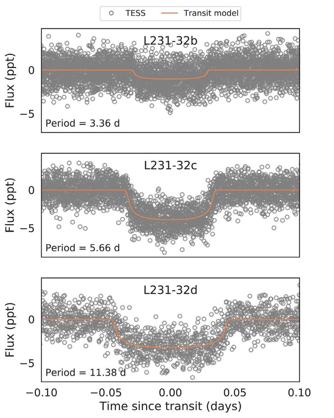
Figure 3. Left. The TESS light curve folded on the orbital period and centred on the mid-transit time for L231-32b (top), L231-32c (middle), and L231-32d
(bottom). The best-fitting model (orange) is shown. Right. The ESPRESSO (green) and HARPS (blue) data folded on the orbital period for L231-32b (top),
L231-32c (middle), and L231-32d (bottom). The best-fitting model (orange) is shown.
Grimm et al. 2018). Subsequently, L231-32b is now the lowest mass of models, in which these two outer planets consist not only of a
exoplanet with masses and radii known to better than 20 per cent core, but also of a low-density envelope. This atmosphere, which
with a mass measured through RV observations. In the range of Mp may consist of H-He, can significantly increase the size of a planet
< 3 M⊕ , there are eight other planets with precisely known masses even if its contribution to its mass is only minor. In Fig. 4, we
and radii; in order of increasing mass they are GJ 1132b (Berta- show composition models (again taken from Zeng et al. 2019) for
Thompson et al. 2015; Bonfils et al. 2018), LHS 1140c (Dittmann an Earth-like core composition (i.e. consistent with the composition
et al. 2017; Lillo-Box et al. 2020), GJ 3473b (Kemmer et al. 2020), of L231-32b), as well as a mass fraction of 1 per cent or 2 per cent
Kepler-78b (Howard et al. 2013; Pepe et al. 2013), GJ 357 b (TOI- H-He.12 These composition models are sensitive to the effective
562; Jenkins et al. 2019; Luque et al. 2019), LTT 3780b (TOI-732; temperature of the planet. We show models for 300, 500, and 700 K,
Cloutier et al. 2020a; Nowak et al. 2020), L98-59c (TOI-175; Cloutier as the size of the planet is sensitive to the temperature for a fixed
et al. 2019; Kostov et al. 2019), and K2-229b (Santerne et al. 2018; core and atmosphere composition. For L231-32c and L231-32d, we
Dai et al. 2019). We zoom in on these small planets in Fig. 5. From this estimate equilibrium temperatures (Teq ) of 447 ± 11 and 354 ± 8 K,
figure, it is clear that all these planets have a relatively high density, respectively, assuming an albedo (Ab) of 0.3. As the equilibrium
and appear to have a strikingly similar composition, consistent with temperature is sensitive to the (unknown) albedo, the true uncertainty
models with a core composition mixture of MgSiO3 and Fe, similar is significantly larger, e.g. for Ab = 0, we have Teq = 488 ± 12
to Earth, even if some may have a slightly denser (more Iron) or lower and Teq = 387 ± 10 for L231-32c and L231-32d, respectively (see
density (more rocky) composition. However, all of these planets are Table 1). We find that L231-32c and L231-32d are broadly consistent
inconsistent with lower density compositions, such as that of pure with models in which their core composition is the same as that of
water planets or planets with even a small mass fraction of H-He L231-32b (i.e. Earth-like rocky), with the addition of an atmosphere
atmosphere. taking up about 1 per cent of the total mass of the planets, where
Unlike the TRAPPIST-1 system, where all seven planets have a the precise mass of the H-He envelope is sensitive to assumptions
similar high density, for L231-32 there is a remarkable difference about the exact core composition and equilibrium temperature of
between the density of L231-32b on the one hand, and that of these planets. In Section 6.2, we investigate the physical mechanisms
L231-32c and L231-32d on the other. Unlike L231-32b, the two that can explain the respective locations of L231-32b, c, and d on the
other planets are inconsistent with an Earth-like rocky composition.
Instead, when assuming a simple core composition model, the lower
density of these planets implies a model such as that of pure water, 12 Theseatmosphere models are referred to as containing H2 by Zeng et al.
but it is hard to find a plausible physical reason for why three
(2019), but are identical to what is referred to as H-He atmospheres in
planets in near-resonant orbits would have formed with such widely photoevaporation models (e.g. Owen & Wu 2013). Namely, both contain
different core compositions. We therefore consider an alternative set a mixture of H2 and He. Here, we use the H-He nomenclature.
MNRAS 507, 2154–2173 (2021)2162 V. Van Eylen et al.
Downloaded from https://academic.oup.com/mnras/article/507/2/2154/6356971 by guest on 17 September 2021
Figure 4. Mass-radius diagram. The planets orbiting L231-32 are indicated in red. Other planets with masses and radii measured to better than 20 per cent (and
R < 3 R⊕ and M < 10 M⊕ ) are shown in grey, with values taken from TEPcat (see Section 5 for details). Theoretical lines indicate composition models. The
solid lines show models for cores consisting of pure Iron (100 per cent Fe), Earth-like rocky (32.5 per cent Fe, 67.5 per cent MgSiO3 ), Half-Rock Half-Iron
(50 per cent Fe, 50 per cent MgSiO3 ), and pure Rock (100 per cent MgSiO3 ). A ‘pure water’ model is also shown. In dashed, dotted, and solid lines, models
with an Earth-like rocky core and an envelope of H-He taking up 1 per cent or 2 per cent of the mass are shown, for temperatures of 300, 500, and 700 K. All
composition models are taken from Zeng et al. (2019). L231-32b is consistent with an Earth-like composition (without a significant envelope). We consider
it most likely that L231-32c and L231-32d consist of an Earth-like core composition and a H2 envelope of about 1 per cent of the planet’s total mass, with
equilibrium temperatures of around 500 and 300 K, respectively.
mass-radius diagram in terms of the presence of an H-He atmosphere We consider transmission spectroscopy for the sub-Neptunes, as
for the outer planets, and the absence of such an atmosphere for the their low densities make them suitable targets for this type of observa-
inner planet. tion. Of the sub-Neptunes with radii 1.8–4 R⊕ and published masses,
L231-32c and L231-32d rank among the most favourable targets (top
panel of Fig. 6). Indeed, simulations for L231-32c and L231-32d have
5.2 Atmospheric studies of L231-32’s planets already shown them to be prime targets for atmospheric studies using
L231-32c and L231-32d are exciting targets for atmospheric studies JWST (Chouqar et al. 2020). Our new mass determinations rule out
for several reasons. First, as we have shown here, L231-32c and a water-dominated atmosphere scenario, significantly decreasing the
L231-32d likely have a significant atmosphere, and determining expected number of transit observations necessary for molecular
their atomic and molecular composition will help interpret the detections, and Chouqar et al. (2020) estimate that fewer than
evolution history of these planets. L231-32 is an M3V star, with three transits with NIRISS and NIRSpec may be enough to reveal
a radius of 0.38 R , which results in relatively deep transits even for molecular features for clear H-He-rich atmospheres.
small planets, making them more feasible for atmospheric studies Meanwhile, the super-Earths with radii 5 mag was applied, as it will be challenging to observe targets or higher ESM values. This raises the likelihood that if L231-32b
brighter than this with JWST (e.g. Beichman et al. 2014) or using possesses an outgassed atmosphere with a high mean molecular
multi-object spectroscopy with large ground-based telescopes such weight, it may have avoided photoevaporative loss, increasing its
as VLT (e.g. Nikolov et al. 2018). appeal as a potential rocky target for JWST follow-up observations.
MNRAS 507, 2154–2173 (2021)L231-32 and the M dwarf radius valley 2163
Downloaded from https://academic.oup.com/mnras/article/507/2/2154/6356971 by guest on 17 September 2021
Figure 5. Mass-radius diagram for Earth-mass planets. This figure is similar to Fig. 4, but zoomed in on planets with M < 3M⊕ . Only a small number of small plan-
ets have masses measured to better than 20 per cent. The seven least massive planets all orbit TRAPPIST-1, and their masses were determined through TTVs. The
other planets, in order of increasing mass, are L231-32b, GJ 1132b, LHS 1140c, GJ 3473b, Kepler-78b, GJ 357b, LTT 3780b, L98-59c, and K2-229b. Their masses
were determined through RVs. All of these planets follow relatively similar composition tracks, consistent with a composition similar to that of Earth, or slightly
more dense (more Iron) or less dense (more Rock). Unlike the other two planets orbiting L231-32, i.e. L231-32c and L231-32d, none of these planets have a low
density, and they are all inconsistent with a composition of a pure water planet or compositions that would include the presence of a significant H-He atmosphere.
5.3 Transit timing variations systems that are either all water-poor or water-rich (Bitsch, Raymond
& Izidoro 2019; Izidoro et al. 2021); only in rare cases where initial
As outlined in Günther et al. (2019), the two outer detected planets,
formation straddled the water snow-line could systems with inner
L231-32c and L231-32d, are expected to produce measurable TTVs
rocky planets and outer water-rich planets be formed (Raymond et al.
due to their proximity to 5 to 3 (planet c to b) and 2 to 1 (planet d to c)
2018). Alternatively, a model in which L231-32c and L231-32d have
resonant configurations. The expected TTV period is approximately
a similar, Earth-like rocky, core composition as L231-32b can match
1100 d (Günther et al. 2019). Further transit observations using other
its locations in the mass-radius diagram, if one is willing to assume
ground-based or space-based instruments may help constrain the
they contain a H-He atmosphere. These atmospheres do not need to
TTV signal of these planets (Kaye et al., in preparation). Such
be very massive, with a H-He atmosphere of about 1 per cent of the
TTV measurements may further refine the planet masses, as well
total planet mass sufficient to explain its mass and radius, as even
as constrain the orbital eccentricities and arguments of pericentre.
a tiny mass fraction of a H-He atmosphere significantly increases
the planet size (see Fig. 4). The exact planet size for a given H-He
envelope mass fraction depends on the temperature of the planet,
6 T H E R A D I U S VA L L E Y F O R M DWA R F S TA R S a quantity which is generally unknown, as it depends on a planet’s
albedo, which is typically unknown.
6.1 The three planets orbiting L231-32 and the radius valley A bimodality in the size and composition of small planets has
As seen in Fig. 4, L231-32b is consistent with a rocky composition been predicted as a consequence of photoevaporation in which some
without any significant atmosphere. The density of L231-32c and planets can lose their entire atmosphere, while others hold on to a
L231-32d is significantly lower. This may suggest a much lower H-He envelope (e.g. Lopez & Fortney 2013; Owen & Wu 2013).
density core, such as a pure water planet, or a core composition Planets with a H-He atmosphere, often called sub-Neptunes, are
similar to that of L231-32b with a H-He atmosphere. Here, we argue significantly larger in size, than stripped core planets that have
that the latter scenario naturally explains the masses and radii of the lost their atmosphere, i.e. the super-Earths. A valley in the radius
three planets orbiting L231-32, and that L231-32b likely formed with distribution separating these two types of planets has been observed
an initial H-He envelope similar to that of the two other planets, but at about 1.6 R⊕ (e.g. Fulton et al. 2017; Berger et al. 2018; Fulton
that this atmosphere has been lost so that only a stripped core remains. & Petigura 2018; Van Eylen et al. 2018). The valley’s exact location
Although the existence of water worlds has been advocated (e.g. is a function of orbital period (Van Eylen et al. 2018) and may
Zeng et al. 2019), it is unlikely that the three planets close to be largely devoid of planets (Van Eylen et al. 2018; Petigura 2020).
mean-motion resonances have different compositions. Specifically, Alternative interpretations of the radius valley have been put forward,
population synthesis models tend to favour the formation of resonant such as a ‘core-powered mass-loss’ scenario in which atmosphere
MNRAS 507, 2154–2173 (2021)2164 V. Van Eylen et al.
Wu 2017). This is consistent with the observation of L231-32c and
L231-32d, the size of which indicates they are sub-Neptunes, located
on the upper side of the radius valley.
We can further check whether the masses and radii of L231-32’s
planets are quantitatively consistent with photoevaporation models,
in terms of which planets could have lost their atmospheres based on
the star’s history of XUV flux. However, as this XUV history is not
well understood, we can instead use the relative composition of the
three planets in this system. Under photoevaporation models, L231-
32b is assumed to have lost its entire initial atmosphere, based on
which we can calculate a minimum mass required for L231-32c and
L231-32d not to have lost their atmospheres. Based on the parameters
and their uncertainties listed in Table 1, we calculate the minimum
Downloaded from https://academic.oup.com/mnras/article/507/2/2154/6356971 by guest on 17 September 2021
mass of L231-32c and L231-32d using the EVAPMASS code13 as
outlined by Owen & Campos Estrada (2020). These minimum
masses answer the question: assuming all planets in the system were
born with H-He atmospheres and that L231-32b was stripped of its
atmosphere, how massive do L231-32c and L231-32d need to be? We
find (at the 95 per cent confidence level) the photoevaporation model
requires L231-32c to be more massive than 1.04 M⊕ and L231-32d to
be more massive than 0.44 M⊕ . These lower limits are not particularly
constraining, and the measured masses are significantly larger than
these masses. This can be understood because XUV irradiation is a
function of orbital period. As a result, a scenario in which the inner
planet loses its atmosphere, while the more distant planets hold on to
theirs, is often (though not always) consistent with photoevaporation.
To summarize, we find here that the mass and radius measurements
of the three planets orbiting L231-32 are consistent with photoevapo-
ration models, in which all three planets started out with a Earth-like
rocky core and a H-He envelope. This envelope was retained by
L231-32c and L231-32d, but stripped away for L231-32b, placing
these planets on opposite ‘banks’ of the radius valley. In Section 6.2,
we investigate what photoevaporation and core-powered mass-loss
Figure 6. Comparison of L231-32 atmospheric metrics against other known models predict about the location of the M dwarf radius valley, and in
exoplanets with K > 5 mag. The top panel shows the TSM values for
Section 6.3, we test these models by comparing L231-32 with other
sub-Neptunes with radii 1.8–4 R⊕ and published masses, versus planetary
well-studied exoplanets orbiting M dwarf stars and determining the
equilibrium temperature. L231-32c and L231-32d rank close to the top of
all known sub-Neptunes and are currently the most favourable known targets location of the M dwarf radius valley.
with equilibrium temperatures below 600 K. The bottom panel shows the ESM
for super-Earths with radii R < 1.8 R⊕ . This includes validated super-Earths
6.2 Expected location of the M dwarf radius valley
without published masses, as the mass does not affect emission spectroscopy.
Of the super-Earths, L231-32b ranks among the most favourable with We now set out to empirically determine the location of the radius
equilibrium temperatures below 1000 K. valley for planets orbiting M dwarf stars. To do so, we first quantify
where models predict the M dwarf radius valley to be. Assuming
loss of planets is driven by the luminosity of the cooling planet the photoevaporation model, we can estimate the position of the
core (e.g. Ginzburg, Schlichting & Sari 2018; Gupta & Schlichting the upper edge of the super-Earths (i.e. the ‘lower boundary’ of the
2020). In this scenario, the physical mechanism for atmosphere loss radius gap). Following Owen & Wu (2017), Owen & Adams (2019),
is different, but as in the photoevaporation scenario the result is and Mordasini (2020), this upper-edge of super-Earths is given by
a population of stripped core, super-Earth planets that have lost the maximum core size for which photoevaporation can strip away
their atmospheres, which is separated by a radius valley from sub- the atmosphere at that orbital period. This maximum core size can
Neptunes, which held on to a H-He envelope. be found by equating the mass-loss time-scale tṁ to the saturation
The location and slope of the radius valley as observed by Van time-scale of the high-energy output of the star tsat ; adopting energy-
Eylen et al. (2018) is consistent with models suggesting planets limited mass-loss we find (equation 27 of Owen & Wu 2017):
below the radius valley are stripped cores of terrestrial composition,
GMp2 X2 η sat
which have lost their entire atmospheres. Furthermore, the emptiness ∼ L tsat (4)
of the valley would suggest a homogeneity in core composition (e.g. 8π Rc3 ap2 HE
Owen & Wu 2017). This appears to be what is observed. L231-32b, with ap the planet’s semimajor axis, η the mass-loss efficiency, X2
the size of which suggests it is a super-Earth, located below the the envelope mass-fraction that doubles the core’s radius (this is,
valley, is consistent with a terrestrial composition, as are other low- approximately, the envelope which is hardest for photoevaporation
mass planets in the mass-radius diagram (see Fig. 5). On the other to strip), and Lsat
HE , the high energy luminosity of star in the saturated
hand, planets with a size on the other side of the valley are predicted
to contain a significant H-He atmosphere, which roughly doubles
their size but contributes only a small amount of mass (e.g. Owen & 13 https://github.com/jo276/EvapMass
MNRAS 507, 2154–2173 (2021)You can also read