LEARNING INVARIANT REPRESENTATIONS AND RISKS FOR SEMI-SUPERVISED DOMAIN ADAPTATION - OpenReview
←
→
Page content transcription
If your browser does not render page correctly, please read the page content below

Under review as a conference paper at ICLR 2021

L EARNING I NVARIANT R EPRESENTATIONS AND R ISKS
FOR S EMI - SUPERVISED D OMAIN A DAPTATION

 Anonymous authors
 Paper under double-blind review

                                            A BSTRACT

         The success of supervised learning hinges on the assumption that the training
         and test data come from the same underlying distribution, which is often not
         valid in practice due to potential distribution shift. In light of this, most existing
         methods for unsupervised domain adaptation focus on achieving domain-invariant
         representations and small source domain error. However, recent works have shown
         that this is not sufficient to guarantee good generalization on the target domain,
         and in fact, is provably detrimental under label distribution shift. Furthermore, in
         many real-world applications it is often feasible to obtain a small amount of labeled
         data from the target domain and use them to facilitate model training with source
         data. Inspired by the above observations, in this paper we propose the first method
         that aims to simultaneously learn invariant representations and risks under the
         setting of semi-supervised domain adaptation (Semi-DA). First, we provide a finite
         sample bound for both classification and regression problems under Semi-DA. The
         bound suggests a principled way to obtain target generalization, i.e. by aligning
         both the marginal and conditional distributions across domains in feature space.
         Motivated by this, we then introduce the LIRR algorithm for jointly Learning
         Invariant Representations and Risks. Finally, extensive experiments are conducted
         on both classification and regression tasks, which demonstrates LIRR consistently
         achieves state-of-the-art performance and significant improvements compared with
         the methods that only learn invariant representations or invariant risks.

1   I NTRODUCTION

The success of supervised learning hinges on the key assumption that test data should share the
same distribution with the training data. Unfortunately, in most of the real-world applications, data
are dynamic, meaning that there is often a distribution shift between the training (source) and test
(target) domains. To this end, unsupervised domain adaptation (UDA) methods aim to approach
this problem by adapting the predictive model from labeled source data to the unlabeled target data.
Recent advances in UDA focus on learning domain-invariant representations that also lead to a small
error on the source domain. The goal is to learn representations, along with the source predictor,
that can generalize to the target domain Long et al. (2015); Ganin et al. (2016); Tzeng et al. (2017);
Long et al. (2018); Chen et al. (2019); Zhao et al. (2018). However, recent works Zhao et al. (2019a);
Wu et al. (2019); Combes et al. (2020) have shown that the above conditions are not sufficient to
guarantee good generalizations on the target domain. In fact, if the marginal label distributions are
distinct across domains, the above method provably hurts target generalization Zhao et al. (2019a).
On the other hand, while labeled target data is usually more difficult or costly to obtain than labeled
source data, it can lead to better accuracy Hanneke & Kpotufe (2019). Furthermore, in many practical
applications, e.g., vehicle counting, object detection, speech recognition, etc., it is often feasible to
at least obtain a small amount of labeled data from the target domain so that it can facilitate model
training with source data Li & Zhang (2018); Saito et al. (2019). Motivated by these observations,
in this paper we focus on a more realistic setting of semi-supervised domain adaptation (Semi-DA).
In Semi-DA, in addition to the large amount of labeled source data, the learner also has access to
a small amount of labeled data from the target domain. Again, the learner’s goal is to produce a
hypothesis that well generalizes to the target domain, under the potential shift between the source
and the target. Semi-DA is both a more-realistic and generalizable setting that allows practitioners to

                                                   1
Under review as a conference paper at ICLR 2021

                                                                                       Source/Target labeled data
                                                                                           Target unlabeled data

                                        Target                     Target
                                        Optimal                    Optimal
                                        Predictor                  Predictor
                                                                           Source
                                                                           Optimal                  Invariant
 Source                                                                    Predictor                Optimal
 Optimal
                                                                                                    Predictor
 Predictor

                                         Invariant                    Invariant
                                       Representations                  Risks

Figure 1: Overview of the proposed model. Learning invariant representations induces indistinguish-
able representations across domains, but there can still be mis-classified samples (as stated in red
circle) due to misaligned optimal predictors. Besides learning invariant representations, LIRR model
jointly learns invariant risks to better align the optimal predictors across domains.

design better algorithms that can overcome the aforementioned limitations in UDA. The key question
in this scenario is: how to maximally exploit the labeled target data for better model training?
In this paper, we address the above question under the Semi-DA setting. In order to first understand
how performance discrepancy occurs, we derive a finite-sample generalization bound for both clas-
sification and regression problems under Semi-DA. Our theory shows that, for a given predictor,
the accuracy discrepancy between two domains depends on two terms: (i) the distance between
the marginal feature distributions, and (ii) the distance between the optimal predictors from source
and target domains. Our observation naturally leads to a principled way of learning invariant repre-
sentations (to minimize discrepancy between marginal feature distributions) and risks (to minimize
discrepancy between conditional distributions over the features) across domains simultaneously for
a better generalization on the target. In light of this, we introduce our novel bound minimization
algorithm LIRR, a model of jointly Learning Invariant Representations and Risks for such purposes.
As a comparison, existing works on focus on either learning invariant representations only Ganin
et al. (2016); Tzeng et al. (2017); Zhao et al. (2018); Chen et al. (2019), or learning invariant risks
only Arjovsky et al. (2019); Chang et al. (2020); Song et al. (2019); Steinberg et al. (2020); Krueger
et al. (2020); Zhao et al. (2020), which are not sufficient to reduce the accuracy discrepancy for good
generalizations on the target. To our best knowledge, LIRR is the first work that subtly combine above
learning objectives with sound theoretical proof and interpretation. LIRR jointly learns invariant
representations and risks, and as a result, better mitigates the accuracy discrepancy across domains.
To better understand our method, we illustrate the proposed algorithm, LIRR, in Fig. 1.
In summary, our work provides the following contributions:

• Theoretically, we provide finite-sample generalization bounds for Semi-DA on both classification
  (Theorem 3.1) and regression (Theorem 3.2) problems. Our bounds inform new directions for
  simultaneously optimizing both marginal and conditional distributions across domains for better
  generalization on the target. To the best of our knowledge, this is the first generalization analysis
  in the Semi-DA setting.
• To bridge the gap between theory and practice, we provide an information-theoretic interpretation
  of our theoretical results. Based on this perspective, we propose a bound minimization algorithm,
  LIRR, to jointly learn invariant representations and invariant optimal predictors, in order to mitigate
  the accuracy discrepancy across domains for better generalizations.
• We systematically analyze LIRR with extensive experiments on both classification and regression
  tasks. Compared with methods that only learn invariant representations or invariant risks, LIRR
  demonstrates significant improvements on Semi-DA. We also analyze the adaptation performance
  with increasing labeled target data, which shows LIRR even surpasses oracle method Full Target
  trained only on labeled target data, suggesting that LIRR can successfully exploit the structure in
  source data to improve generalization on the target domain.

                                                    2
Under review as a conference paper at ICLR 2021

2    P RELIMINARIES

Unsupervised Domain Adaptation We use X and Y to denote the input and output space, respec-
tively. Similarly, Z stands for the representation space induced from X by a feature transformation
g : X 7→ Z. Accordingly, we use X, Y, Z to denote random variables which take values in X , Y, Z.
Throughout the paper, a domain corresponds to a joint distribution on the input space X and output
space Y. We use DS (DT ) to denote the source (target) domain and subsequently we also use
DS (Z)(DT (Z)) to denote the marginal distributions of DS (DT ) over Z. Furthermore, let D be a
categorical variable that corresponds to the index of domain, i.e., D ∈ {S, T }. The overall sampling
process for our data can then be specified by first drawing a value of D, and then depending on the
value of D, we sample from the corresponding distribution DD . Under this setting, the probabilities
of Pr(D = T ) and Pr(D = S) then determine the relative sample sizes of our target and source data.
A hypothesis is a function h : Z → [0, 1]. The error of a hypothesis h under distribution DS and
feature transformation g is defined as: εS (h, f ) := EDS [|h(g(X)) − f (X)|]. In classification setting,
in which f and h are binary classification functions, above definition reduces to the probability
that h disagrees with f under DS : EDS [|h(g(X)) − f (X)|] = EDS [I(h(g(X)) 6= f (X))] =
PrDS (h(g(X)) 6= Y ). In regression, the above error is then the usual mean absolute error, i.e., the
`1 loss. As a common notation, we also use εbS (h) to denote the empirical risk of h on the source
domain. Similarly, εT (h) and εbT (h) are the true risk and the empirical risk on the target domain.

Semi-supervised Domain Adaptation Formally, in Semi-DA the learner is allowed to have access
                                                                    (S) (S)
to a small amount of labeled data in target domain DT . Let S = {(xi , yi )}ni=1 be a set of labeled
                                                          (T )
data sampled i.i.d. from DS . Similarly, we have T = {(xj )}kj=1 as the set of target unlabeled data
                                         (Te) (Te)
sampled from DT , and we let Te = {(xj , yj )}m    j=1 be the small set of labeled data where m ≤ k.
Usually, we also have m  n, and the goal of the learner is to find a hypothesis h ∈ H by learning
from S and T so that h has a small target error εT (h).
Clearly, with the additional small amount of labeled data Te, one should expect a better generalization
performance than what the learner could hope to achieve in the setting of unsupervised domain
adaptation. To this end, we first state the following generalization upper bound from Zhao et al.
(2019a) in the setting of unsupervised domain adaptation:
Theorem 2.1. (Zhao et al., 2019a) Let hDS (X), fS i and hDT (X), fT i be the source and target
domains. For any function class H ⊆ [0, 1]X , and ∀h ∈ H, the following inequality holds:
        εT (h) ≤ εS (h) + dH (DS (X), DT (X)) + min{EDS [|fS − fT |], EDT [|fS − fT |]}.             (1)

The dH (·, ·) is known as the H-divergence (Ben-David et al., 2010), a pseudo-metric parametrized by
H to measure the discrepancy between two distributions. It should be noted that the above theorem
is a population result, hence it does not give a finite sample bound. Furthermore, the setting above
is noiseless, where fS and fT correspond to the groundtruth labeling functions in source and target
domains. Nevertheless, it provides an insight on achieving domain adaptation through bounding the
error difference on source and target domains: to simultaneously minimize the distances between
feature representations and between the optimal labeling functions.

3    G ENERALIZATION B OUNDS FOR S EMI - SUPERVISED D OMAIN A DAPTATION

In this section, we derive a finite-sample generalization bound for Semi-DA, where the model has
access to both a large amount of labeled data S from the source domain, and a small amount of
labeled data T̃ from the target domain. For this purpose, we first introduce the definition of H on both
classification and regression settings, and then present our theoretical results of the generalization
upper bounds for Semi-DA.
Definition 3.1. Let H be a family of binary functions from Z to {0, 1}, and AH be the collection of
subsets of Z defined as AH := {h−1 (1) | h ∈ H}. The distance between two distributions D and D0
based on H is: dH (D, D0 ) := supA∈AH | PrD (A) − PrD0 (A)|.

                                                   3
Under review as a conference paper at ICLR 2021

With the definition, we have the symmetric difference w.r.t. itself as: H∆H = {h(z) ⊕ h0 (z) | h, h0 ∈
H}, where ⊕ is the XOR operation. Next, considering that for a joint distribution D over Z × Y
in our setting, there may be noise in the conditional distribution PrD (Y | Z). It is then necessary
to define a term to measure the noise level of each domain. To this end, in classification, we define
the noise on the source domain nS := ES [|Y − fS (Z)|], where fS : Z → [0, 1] is the conditional
mean function, i.e., fS (Z) = ES [Y | Z]. Similar definition also applies to the target domain, where
we use nT to denote the noise in target. In regression, with `1 loss, we define fS : Z → R to be
the conditional median function of Pr(Y | Z), i.e. fS (Z) := inf y {y ∈ R : 1/2 ≤ Pr(Y ≤ y | Z)}.
Now we are ready to state the main results in this section:
Theorem 3.1. (Classification generalization bound in Semi-DA). Let H be a hypothesis set with
functions h : Z → {0, 1} and V Cdim(H) = d, D       bS (resp. DbT ) be the empirical distribution induced
by samples from DS (resp. DT ). For 0 < δ < 1, then w.p. at least 1 − δ over the n samples in S and
m samples in T̃ , for all h ∈ H, we have:
              m                  n
εT (h) ≤           εbT̃ (h) +         εbS (h)
            n+m               n+m
              n    h                                                                                    i
        +            dH∆H (D  bS (Z), D bT (Z)) + min{ES [|fS (Z) − f (Z)|], ET [|fS (Z) − f (Z)|]}
                                                                       T̃                       T̃
           n+m
                                        r                                      !
              n                             1    1    1    d     n      d    m
        +          |nS + nT̃ | + O         ( + )log + log + log                   .
           n+m                              m n       δ    n     d     m     d

Theorem 3.2. (Regression generalization bound in Semi-DA). Let H be a hypothesis set with
functions h : Z → [0, 1] and P dim(H) = d, D  bS (resp. D
                                                        bT ) be the empirical distribution induced by
samples from DS (resp. DT ). Then we define H̃ := {I|h(x)−h0 (x)|>t : h, h0 ∈ H, 0 ≤ t ≤ 1}. For
0 < δ < 1, then w.p. at least 1 − δ over the n samples in S and m samples in T̃ , for all h ∈ H, we
have:
               m                n
  εT (h) ≤        εb (h) +          εbS (h)
             n + m T̃        n+m
               n  h                                                                               i
         +          dH̃ (D
                         bS (Z), DbT (Z)) + min{ES [|fS (Z) − f (Z)|], ET [|fS (Z) − f (Z)|]}
                                                                  T̃                      T̃
            n+m
                                      r                                       !
               n                          1    1     1    d     n    d     m
         +        |nS + nT̃ | + O        ( + )log + log + log                    .
            n+m                           m n        δ    n     d    m     d

Remark It is worth pointing out that both nS and nT are constants that only depend on the
underlying source and target domains, respectively. Hence |nS + nT | essentially captures the the
amplitude of noise. The last two terms of the bound come from standard concentration analysis for
uniform convergence.
Comparing with previous results Ben-David et al. (2010); Zhao et al. (2019a); Combes et al. (2020);
Redko et al. (2017; 2019), our bounds is the first in Semi-DA literature which contain empirical error
terms from both the source and target domains and replace λ term with our fourth term, which is
tighter since λ relies the choice of the hypothesis class H. More importantly, these bounds imply
a natural and principled way for a better generalization to the target domain by learning invariant
representations and risks simultaneously. Note that this is in sharp contrast to previous works where
only invariant representations are pursued Ganin et al. (2016); Zhao et al. (2018).

4    L EARNING I NVARIANT R EPRESENTATIONS AND R ISKS
Motivated by the generalization error bounds in Thm. 3.1 and 3.2 in Sec. 3, in this section we propose
our bound minimization algorithm LIRR. Since the last two terms reflect the noise level, complexity
measures and error caused by finite samples, respectively, we then hope to optimize the upper bound
by minimizing the first four terms. The first two terms are the convex combination of empirical
errors of h on S and T , which can be optimized with the labeled source and target data. The third
term measures the distance of representations between the source and target domains, which is a
good inspiration for us to learn the invariant representation (Ganin et al., 2016) across domains. The
fourth term corresponds to the distance of the optimal classifiers between S and T . To minimize this

                                                   4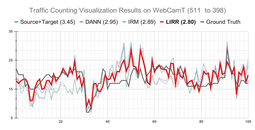
Under review as a conference paper at ICLR 2021

term, the model is forced to learn the data representations that induce the same optimal predictors
for both source and target domains, which exactly corresponds to the principle of invariant risk
minimization (Arjovsky et al., 2019).

4.1   I NFORMATION T HEORETIC I NTERPRETATION

To better understand why the bound minimization strategy can solve the intrinsic problems of
Semi-DA, in what follows we provide interpretations from an information-theoretic perspective.
Invariant Representations Learning invariant representations corresponds to minimizing the third
term of the bound Thm. 3.1 and bound Thm. 3.2. We consider a feature transformation Z = g(X)
that can obtain the invariant representation Z from input X. The invariance on representations can
be described as achieving statistical independence D ⊥ Z, where D stands for the domain index.
This independence is equivalent to the minimization of mutual information I(D; Z). To see this, if
I(D; Z) = 0, then DS (Z) = DT (Z), so the third term in the bounds will vanish. Intuitively, this
means that by looking at the representations Z, even a well-trained domain classifier C(·) cannot
correctly guess the domain index D. We also call the learned feature transformation g : X → Z the
invariant encoder.
Invariant Risks Learning invariant risks corresponds to minimizing the fourth term of the bound
Thm. 3.1 and bound Thm. 3.2. Inspired by Arjovsky et al. (2019), we want to identify a subset
of feature representation through feature transformation Z = g(X) that best supports an invariant
optimal predictor for source and target domains. That means the identified feature representation
Z = g(X) can induce the same optimal predictors. This objective can be interpreted with a
conditional independence D ⊥ Y | Z, which is equivalent to minimizing I(D; Y | Z). To see this,
when the conditional mutual information of I(D; Y | Z) equal 0, the two conditional distributions
PrS (Y | Z) and PrT (Y | Z) coincide with each other. As a result, the optimal predictors become
the same across domains, so the fourth term in our bounds Thm. 3.1, Thm. 3.2 will vanish.
In summary, our learning objective on invariant representations and invariant risks are achievable
with the minimization on I(D; Z) and I(D; Y | Z). It is instructive to present the integrated form
as in Eq. 2. In words, the integrated form suggests the independence of D ⊥ (Y, Z). We regard the
independence as an intrinsic objective for domain adaptation since it implies an alignment of the joint
distributions over (Y, Z) across domains, as opposed to only the marginal distributions over Z.

                           I(D; Y, Z) =         I(D; Z)              + I(D; Y | Z)                 (2)
                                                | {z }                 |   {z    }
                                          Invariant Representation      Invariant Risk

4.2   A LGORITHM D ESIGN

To learn invariant representations, that is achieving marginal independence of Y ⊥ Z and mini-
mization on min I(Y ; Z), we adopt the adversarial training method as in Ganin et al. (2016). The
invariant representation objective focuses on learning the feature transformation g(·) to obtain the
invariant representations from input X, which can fool the domain classifier C. This part of the
objective function can be described as in Eq. 3.
            Lrep (g, C) = EX∼DS (X) [log(C(g(X)))] + EX∼DT (X) [log(1 − C(g(X)))]                  (3)

To learn invariant risks, that is achieving conditional independence of D ⊥ Y | Z, we resort to the
conditional mutual information minimization on I(D; Y | Z), and further convert min I(D; Y | Z)
objective to the minimization of the difference between the two conditional entropies, as in Eq. 4.
                        min I(D; Y | Z) = min H(Y | Z) − H(Y | D, Z)                               (4)
The following proposition gives a variational form of the conditional entropy as infimum over a
family of cross-entropies, where L denotes the cross-entropy loss.
Proposition 4.1. Farnia & Tse (2016) H(Y | Z) = inf f E[L(Y ; f (Z))].

Using the above variational form, the minimization of the conditional entropies could be transformed
to a minimization of the cross-entropy losses of domain-invariant predictor fi and domain-dependent

                                                     5
Under review as a conference paper at ICLR 2021

predictor fd . The learning objective of the two predictors can be shown as in Eq. 5 and Eq. 6,
respectively. Notice that the domain-dependent loss Ld should be no greater than the domain-
invariant loss Li , because of the additional domain information.

                                  min Li = E(x,y)∼DS ,DT̃ [L(y, fi (g(x)))]                              (5)
                                   g,fi

                           min Ld = Ed∼D E(x,y)∼DS ,DT̃ [L(y, fd (g(x), d))]                             (6)
                           g,fd

Hence, the overall learning objective of Eq. 4 can be re-written with the following loss functions.

                                  min max Lrisk = Li + λrisk (Li − Ld )                                  (7)
                                  g,fi    fd

The first term of Eq. 7 regards to the supervised training on source and target labeled data; the second
term regards to approaching the minimization objective of H(Y | Z) − H(Y | D, Z), as well as
achieving the predictions’ invariance between fi and fd over the same representation z. If we take
the example of binary classification of bear and dog as in Eq . 1, if fi and fd have their prediction of
bear according to a proper representation of animal’s shape, then any domain information will not
contribute to the prediction, thus the predictor captures the invariant part and achieves invariant risks.
In general, as the factorization in Eq. 2 suggests, in order to achieve improved adaptation performance
by minimizing the accuracy discrepancy between domains, we need to enforce the joint independence
of (Y, Z) ⊥ D by learning feature transformation g. To achieve it, we propose our learning objective
of LIRR as in Eq. 8, where λrisk and λrep are set to 1 by default.
                  min max LLIRR (g, fi , fd , C) = Lrisk (g, fi , fd ) + λrep Lrep (g, C)                (8)
                  g,fi C,fd

At a high level, the first term Lrisk (g, fi , fd ) in the above optimization formulation stems from the
minimization of I(Y ; D | Z), and the second term Lrep (g, C) is designed to minimize I(D; Z).

5     E XPERIMENTS
In this section, we introduce the experimental settings, results analysis, and ablation study for the
experiments on both classification and regression tasks. More experimental settings, implementation
details, and results are included in the Appendix.

5.1   I MAGE C LASSIFICATION

Datasets: To verify the efficacy of LIRR on the image classification problem, we conduct experiments
on NICO (He et al., 2020), VisDA2017 (Peng et al., 2017), OfficeHome (Venkateswara et al., 2017),
and DomainNet (Peng et al., 2019) datasets. NICO is dedicatedly designed for O.O.D. (out-of-
distribution) image classification. It has two superclasses animal and vehicle, and each superclass
contains different environments1 , e.g. bear on grass or snow. VisDA2017 contains Train (T) domain
and Validation (V) domain with 12 classes in each domain. Office-Home includes four domains:
RealWorld (RW), Clipart (C), Art (A), and Product (P), with 65 classes in each domain. DomainNet
is the largest domain adaptation dataset for image classification with over 600k images from 6
domains: Clipart (C), Infograph (I), Painting (P), Quickdraw (Q), Real (R), and Sketch (S), with 345
classes in each domain. For each dataset, we randomly pick source-target pairs for the evaluation. To
satisfy the setting of Semi-DA, which has access to a few labeled target samples, we randomly select
a small ratio (1% or 5%) of the target data as labeled target samples.
Baselines: We compare our approach with the following representative domain adaptation methods:
DANN (Ganin et al., 2016), CDAN (Long et al., 2018), IRM (Arjovsky et al., 2019), ADR (Saito
et al., 2017), and MME (Saito et al., 2019); S+T, a model trained with the labeled source and the few
labeled target samples without using unlabeled target samples; and Full T, a model trained with the
fully labeled target. All these methods are implemented and evaluated under the Semi-DA setting.
    1
      For animal, we sample 8 classes from environments grass and snow as two domains. For vehicle, we sample
7 classes from environments sunset and beach as two domains.

                                                      6
Under review as a conference paper at ICLR 2021

Table 1: Accuracy (%) comparison (higher means better) on NICO, OfficeHome, DomainNet, and
VisDA2017 with 1% (above) and 5% (below) labeled target data (mean ± std).

1% labeled target         NICO Animal                       NICO Traffic                              OfficeHome                                       Domainnet                          VisDA2017
   Method           Grass to Snow   Snow to Grass   Sunset to Beach   Beach to Sunset   Art to Real   Real to Prod.   Prod. to Clip.   Real to Clip.   Sketch to Real   Clip. to Sketch   Train to Val.
     S+T            70.06±2.14      80.08±1.21       71.37±1.54        70.07±1.28       69.20±0.15    74.63±0.13      48.65±0.12       48.37±0.08      57.44±0.07       44.16±0.05        76.17±0.15
   DANN             83.80±1.73      81.57±1.51       72.69±1.35        72.03±1.05       72.20±0.23    78.13±0.26      52.47±0.21       51.53±0.19      60.23±0.15       46.36±0.15        78.91±0.25
   CDAN             82.33±0.59      78.25±0.74       75.53±0.55        74.31±0.47       72.98±0.33    79.15±0.31      53.80±0.33       50.67±0.25      60.53±0.23       44.66±0.22        80.23±0.41
    ADR             73.06±1.20      76.74±0.89       72.85±0.95        69.47±0.81       70.55±0.27    76.62±0.28      49.47±0.31       49.94±0.21      59.63±0.22       44.73±0.21        80.40±0.36
     IRM            78.55±0.34      78.27±0.51       64.58±2.41        69.10±2.36       71.13±0.25    77.60±0.24      51.53±0.21       51.86±0.13      58.04±0.12       46.96±0.15        80.79±0.27
    MME             87.12±0.76      79.52±0.43       78.69±0.86        74.21±0.78       72.66±0.18    78.07±0.17      52.78±0.16       51.04±0.12      60.35±0.12       45.09±0.14        80.52±0.35
    LIRR            86.80±0.61      84.78±0.53       71.85±0.58        72.04±0.75       73.12±0.19    79.58±0.22      54.33±0.24       52.39±0.15      61.20±0.10       47.31±0.11        81.67±0.22
 LIRR+CosC          89.67±0.72      89.73±0.68       81.00±0.89        79.98±0.95       73.62±0.21    80.20±0.23      53.84±0.19       53.42±0.09      61.79±0.11       47.83±0.10        82.31±0.21
    Full T          94.52±0.74      97.98±0.23       99.80±0.87        97.64±0.96       83.67±0.12    91.42±0.05      78.27±0.23       72.40±0.05      77.11±0.07       62.66±0.07        89.56±0.14
5% labeled target         NICO Animal                       NICO Traffic                              OfficeHome                                       Domainnet                          VisDA2017
   Method           Grass to Snow   Snow to Grass   Sunset to Beach   Beach to Sunset   Art to Real   Real to Prod.   Prod. to Clip.   Real to Clip.   Sketch to Real   Clip. to Sketch   Train to Val.
     S+T            75.83±1.89      83.38±1.23       86.45±1.08        86.13±0.87       72.10±0.13    78.84±0.12      54.51±0.10       59.80±0.13      66.14±0.11       51.71±0.09        82.87±0.12
   DANN             76.13±0.73      84.61±1.21       84.13±1.20        87.50±1.09       75.47±0.22    80.41±0.21      59.37±0.20       61.31±0.14      68.21±0.20       52.78±0.22        83.95±0.10
   CDAN             82.33±0.59      83.08±2.13       86.97±0.47        87.50±0.56       74.92±0.29    80.57±0.33      59.14±0.31       62.18±0.22      68.49±0.19       53.77±0.21        83.31±0.32
    ADR             80.36±0.31      80.97±0.98       84.50±0.91        75.29±0.87       75.47±0.27    79.27±0.26      58.24±0.27       61.22±0.38      67.96±0.37       53.19±0.32        83.57±0.43
     IRM            81.57±1.01      84.29±1.10       85.71±2.20        83.61±2.17       74.71±0.21    79.67±0.25      58.98±0.22       60.69±0.30      67.81±0.28       52.31±0.25        82.62±0.29
    MME             87.80±0.87      85.50±0.95       92.02±0.85        90.76±0.81       75.24±0.22    82.45±0.18      61.75±0.19       62.31±0.11      69.02±0.18       53.88±0.14        84.12±0.22
    LIRR            85.90±0.98      85.24±0.73       90.77±0.42        88.90±0.39       76.14±0.18    83.64±0.21      62.61±0.17       62.74±0.21      69.35±0.13       54.05±0.17        84.47±0.19
 LIRR+CosC          88.97±0.45      88.22±0.55       92.70±0.87        91.50±1.05       76.63±0.19    83.45±0.22      62.84±0.23       63.03±0.17      69.52±0.09       54.44±0.12        85.06±0.17
    Full T          94.52±0.74      97.98±0.23       99.80±0.87        97.64±0.96       83.67±0.12    91.42±0.05      78.27±0.23       72.40±0.05      77.11±0.07       62.66±0.07        89.56±0.14

Table 2: Mean absolute error (MAE, lower means better) comparison on Citycam with 1% and 5%
labeled target data (mean ± std). The best is emphasized in bold.

                                              253 to 398                                     170 to 398                                     511 to 398
                     Method
                                            1%          5%                                 1%          5%                                 1%          5%
                      S+T                3.20±0.03 2.42±0.02                            3.12±0.02 2.07±0.01                            3.45±0.02 2.82±0.04
                     ADDA                3.13±0.01 2.34±0.03                            3.05±0.03 2.05±0.01                            2.87±0.03 2.45±0.02
                     DANN                3.08±0.02 2.38±0.02                            3.01±0.04 2.01±0.02                            2.95±0.03 2.41±0.04
                      IRM                3.11±0.02 2.27±0.03                            2.91±0.02 2.02±0.01                            2.89±0.05 2.33±0.03
                     LIRR                2.96±0.02 2.13±0.01                            2.84±0.01 1.98±0.02                            2.80±0.03 2.25±0.01
                     Full T              1.68±0.01 1.68±0.01                            1.68±0.01 1.68±0.01                            1.68±0.01 1.68±0.01

5.2       T RAFFIC C OUNTING R EGRESSION

Datasets: To verify the efficacy of LIRR on the regression problem, we conduct experiments on
WebCamT dataset (Zhang et al., 2017) for the Traffic Counting Regression task. WebCamT has
60,000 traffic video frames annotated with vehicle bounding boxes and counts, collected from 16
surveillance cameras with different locations and recording time. We pick three source-target pairs
with different visual similarities: 253→398, 170→398, 511→398 (digit denotes camera ID).
Baselines: The baseline models for this task are generally aligned with our classification experiments
except the methods that can not be applied to the regression task (e.g. MME, ADR, and CDAN).
Thus, for the traffic counting regression task, we compare with the baseline methods: ADDA (Tzeng
et al., 2017), DANN, IRM, S+T, and FullT.

5.3       E XPERIMENTAL R ESULTS A NALYSIS

The classification results are shown in Table 1 with 1% and 5% labeled target data. LIRR outper-
forms the baselines on all the five adaptation datasets, which consistently indicates its effectiveness.
As our learning objective suggests, LIRR can be viewed as achieving D ⊥ (Y, Z), which combines
the benefits of achieving D ⊥ Y and D ⊥ Y | Z. In contrast, DANN, CDAN, and ADDA can be
viewed as only achieving D ⊥ Z or its variant form; and IRM can be viewed as an approximation to
achieve D ⊥ Y | Z using gradient penalty. LIRR outperforms all these methods on different datasets
with 1% or 5% labeled target data, demonstrating simultaneously learning invariant representations
and risks achieves better generalization for domain adaptation than only learning one of them. Such
results are consistent with our theoretical analysis and algorithm design objective. Besides, when
applying LIRR along with the cosine classifier (CosC) module, which is also used in MME, the
performance further outperforms MME by a larger margin.
The traffic counting regression results are shown in Table 2 with 1% and 5% labeled target data.
The superiority of LIRR over baseline methods is supported by its lowest MAE on all the settings.

                                                                                                 7
Under review as a conference paper at ICLR 2021
Officehome-Art to RealWorld
S+T ADR IRM DANN CDAN MME LiRR LiRR + CosC Full Target
87.41
87.02
85.15
84.71
84.17
83.94
Training with
83.67
83.67
83.67
83.67
83.67
83.67
83.67
83.63
83.32
83.24
83.07
83.6
82.84
82.62
82.63
full target
82.45
82.39
82.16
82.07
81.83
81.75
81.77
81.52
81.44
labeled data
81.6
81.6
80.83
80.67
80.52
80.51
80.06
79.74
79.59
79.19
78.8
77.95
77.88
76.63
76.35
76.8
76.14
75.87
75.47
75.47
Acc
75.24
74.92
74.71
74.63
73.62
73.12
72.98
72.66
72.2
72.1
71.13
70.55
69.2
1% 5% 10% 15% 20% 25% 30%
Target label amount
Figure 2: Performance comparison with increasing number of labeled target data, from Domain Art
to RealWorld on Officehome dataset. X axis: the ratio of labeled target data; Y axis: accuracy.
DANN and ADDA are the representative methods of learning invariant representations, while IRM
is the representative method of learning invariant risks. Both DANN, ADDA, and IRM achieve
lower error than S+T, which means learning invariant representations or invariant risks can benefit
Semi-DA to some extent on the regression task. Similar with the observations from the classification
experiments, LIRR outperforms both DANN, ADDA, and IRM, demonstrating simultaneously
learning invariant representations and risks achieves better adaptation than only aligning one of them.
5.4 A BLATION S TUDY
Comparisons with optimizing single invariant objective. As pointed out in Sec. 5.3, LIRR is
simultaneously learning invariant representations and risks, while DANN, CDAN, ADDA can be
viewed as only achieving invariant representations or its variant forms, and IRM is an approximation
to solely achieve invariant risks. From the results on both classification and regression tasks, we can
further acknowledge the importance of simultaneously optimizing these two invariant items together.
As shown in Table 1 and 2, all the methods that only minimize one single invariant objective perform
worse than LIRR, indicating our method is effective and consistent to the theoretical results.
Increasing proportions of labeled target data. Revisiting Thm. 3.1 and Thm. 3.2, we know that as
the proportion of the labeled target data rises, the upper bound of T (h) gets tighter. Accordingly,
the margin between LIRR and other methods becomes larger, as shown in Fig. 2. Another riveting
observation from Fig. 2 is, LIRR and its variant LIRR+CosC even achieve better performance than
the oracle by large margin with 25% or 30% labeled target data. Stunning but plausible, with source
and a few labeled target data, LIRR can learn more robust and generalized representations and achieve
better performance on the target, comparing with the model trained by the fully labeled target data.
Cosine Classifier. As introduced in Saito et al. (2019), cosine classifier is proved to be helpful for
improving the model’s performance on Semi-DA. As shown in Table. 1, the same phenomenon can
be found when comparing the performance of LIRR and LIRR+CosC. For almost all the cases, LIRR
plus cosine classifier module achieves higher accuracy than LIRR alone.
6 R ELATED W ORK
Domain Adaptation Most existing research on domain adaptation focuses on the unsupervised
setting, i.e. the data from target domain are fully unlabeled. Recent deep unsupervised domain
adaptation (UDA) methods usually employ a conjoined architecture with two streams to represent the
models for the source and target domains, respectively (Zhuo et al., 2017). Besides the task loss on
the labeled source domain, another alignment loss is designed to align the source and target domains,
such as discrepancy loss (Long et al., 2015; Sun et al., 2016; Zhuo et al., 2017; Adel et al., 2017;
Kang et al., 2019; Chen et al., 2020), adversarial loss (Bousmalis et al., 2017; Tzeng et al., 2017;
Shrivastava et al., 2017; Russo et al., 2018; Zhao et al., 2019b), and self-supervision loss (Ghifary
8
Under review as a conference paper at ICLR 2021

et al., 2015; 2016; Bousmalis et al., 2016; Carlucci et al., 2019; Feng et al., 2019; Kim et al., 2020;
Mei et al., 2020). Semi-DA deals with the domain adaptation problem where some target labels are
available (Donahue et al., 2013; Li et al., 2014; Yao et al., 2015; Ao et al., 2017). Saito et al. (2019)
empirically observed that UDA methods often fail in improving accuracy in Semi-DA and proposed a
min-max Entropy approach that adversarially optimizes an adaptive few-shot model. Different from
these works, our proposed method aims to align both the marginal feature distributions as well as the
conditional distributions of the label over the features, which can arguably overcome the limitations
that exist in UDA methods that only align feature distributions (Zhao et al., 2019a; Wu et al., 2019).

Invariant Risk Minimization In a seminal work, Arjovsky et al. (2019) consider the question that
data are collected from multiple envrionments with different distributions where spurious correlations
are due to dataset biases. This part of spurious correlation will confuse model to build predictions
on unrelated correlations (Lake et al., 2017; Janzing & Scholkopf, 2010; Schölkopf et al., 2012)
rather than true causal relations. IRM (Arjovsky et al., 2019) estimates invariant and causal variables
from multiple environments by regularizing on predictors to find data represenation matching for all
environments. Chang et al. (2020) extends IRM to neural predictions and employ the environment
aware predictor to learn a rationale feature encoder. As a comparison, in this work we provably show
that IRM is not sufficient to ensure reduced accuracy discrepancy across domains, and we propose to
align the marginal features as well simultaneously.

7   C ONCLUSION

Compared with UDA, the setting of semi-DA is more realistic and has broader practical applications.
In this paper we propose finite-sample generalization bounds for both classification and regression
problems under Semi-DA. Our results shed new light on Semi-DA by suggesting a principled
way of simultaneously learning invariant representations and risks across domains, leading to the
bound minimization algorithm - LIRR. Extensive experiments on real-world datasets, including both
image classification and traffic counting tasks, demonstrate the effectiveness of LIRR as well as its
consistency to our theoretical results.

R EFERENCES
Tameem Adel, Han Zhao, and Alexander Wong. Unsupervised domain adaptation with a relaxed
  covariate shift assumption. In Thirty-First AAAI Conference on Artificial Intelligence, 2017.

Shuang Ao, Xiang Li, and Charles X Ling. Fast generalized distillation for semi-supervised domain
  adaptation. In AAAI Conference on Artificial Intelligence, 2017.

Martin Arjovsky, Léon Bottou, Ishaan Gulrajani, and David Lopez-Paz. Invariant risk minimization.
 arXiv preprint arXiv:1907.02893, 2019.

Shai Ben-David, John Blitzer, Koby Crammer, Alex Kulesza, Fernando Pereira, and Jennifer Wortman
  Vaughan. A theory of learning from different domains. Machine learning, 79(1-2):151–175, 2010.

John Blitzer, Koby Crammer, Alex Kulesza, Fernando Pereira, and Jennifer Wortman. Learning
  bounds for domain adaptation. In Advances in neural information processing systems, pp. 129–136,
  2008.

Konstantinos Bousmalis, George Trigeorgis, Nathan Silberman, Dilip Krishnan, and Dumitru Erhan.
  Domain separation networks. In Advances in Neural Information Processing Systems, pp. 343–351,
  2016.

Konstantinos Bousmalis, Nathan Silberman, David Dohan, Dumitru Erhan, and Dilip Krishnan.
  Unsupervised pixel-level domain adaptation with generative adversarial networks. In IEEE
  Conference on Computer Vision and Pattern Recognition, pp. 3722–3731, 2017.

Fabio M Carlucci, Antonio D’Innocente, Silvia Bucci, Barbara Caputo, and Tatiana Tommasi. Domain
  generalization by solving jigsaw puzzles. In Proceedings of the IEEE Conference on Computer
  Vision and Pattern Recognition, pp. 2229–2238, 2019.

                                                   9
Under review as a conference paper at ICLR 2021

Shiyu Chang, Yang Zhang, Mo Yu, and Tommi S Jaakkola. Invariant rationalization. arXiv preprint
  arXiv:2003.09772, 2020.
Chao Chen, Zhihang Fu, Zhihong Chen, Sheng Jin, Zhaowei Cheng, Xinyu Jin, and Xian-Sheng
  Hua. Homm: Higher-order moment matching for unsupervised domain adaptation. arXiv preprint
  arXiv:1912.11976, 2019.
Chao Chen, Zhihang Fu, Zhihong Chen, Sheng Jin, Zhaowei Cheng, Xinyu Jin, and Xian-Sheng Hua.
  Homm: Higher-order moment matching for unsupervised domain adaptation. In AAAI Conference
  on Artificial Intelligence, 2020.
Remi Tachet des Combes, Han Zhao, Yu-Xiang Wang, and Geoff Gordon. Domain adaptation with
  conditional distribution matching and generalized label shift. arXiv preprint arXiv:2003.04475,
  2020.
Jeff Donahue, Judy Hoffman, Erik Rodner, Kate Saenko, and Trevor Darrell. Semi-supervised
  domain adaptation with instance constraints. In IEEE Conference on Computer Vision and Pattern
  Recognition, pp. 668–675, 2013.
Farzan Farnia and David Tse. A minimax approach to supervised learning. In Advances in Neural
  Information Processing Systems, pp. 4240–4248, 2016.
Zeyu Feng, Chang Xu, and Dacheng Tao. Self-supervised representation learning from multi-domain
  data. In IEEE International Conference on Computer Vision, pp. 3245–3255, 2019.
Yaroslav Ganin, Evgeniya Ustinova, Hana Ajakan, Pascal Germain, Hugo Larochelle, François
  Laviolette, Mario Marchand, and Victor Lempitsky. Domain-adversarial training of neural networks.
  The Journal of Machine Learning Research, 17(1):2096–2030, 2016.
Muhammad Ghifary, W Bastiaan Kleijn, Mengjie Zhang, and David Balduzzi. Domain generalization
 for object recognition with multi-task autoencoders. In Proceedings of the IEEE international
 conference on computer vision, pp. 2551–2559, 2015.
Muhammad Ghifary, W Bastiaan Kleijn, Mengjie Zhang, David Balduzzi, and Wen Li. Deep
 reconstruction-classification networks for unsupervised domain adaptation. In European Confer-
 ence on Computer Vision, pp. 597–613, 2016.
Steve Hanneke and Samory Kpotufe. On the value of target data in transfer learning. In Advances in
  Neural Information Processing Systems, pp. 9871–9881, 2019.
Yue He, Zheyan Shen, and Peng Cui. Towards non-iid image classification: A dataset and baselines.
  Pattern Recognition, pp. 107383, 2020.
Dominik Janzing and Bernhard Scholkopf. Causal inference using the algorithmic markov condition.
  IEEE Transactions on Information Theory, 56(10):5168–5194, 2010.
Guoliang Kang, Lu Jiang, Yi Yang, and Alexander G Hauptmann. Contrastive adaptation network for
  unsupervised domain adaptation. In IEEE Conference on Computer Vision and Pattern Recognition,
  pp. 4893–4902, 2019.
Donghyun Kim, Kuniaki Saito, Tae-Hyun Oh, Bryan A Plummer, Stan Sclaroff, and Kate
  Saenko. Cross-domain self-supervised learning for domain adaptation with few source labels.
  arXiv:2003.08264, 2020.
David Krueger, Ethan Caballero, Joern-Henrik Jacobsen, Amy Zhang, Jonathan Binas, Remi Le Priol,
  and Aaron Courville. Out-of-distribution generalization via risk extrapolation (rex). arXiv preprint
  arXiv:2003.00688, 2020.
Brenden M Lake, Tomer D Ullman, Joshua B Tenenbaum, and Samuel J Gershman. Building
  machines that learn and think like people. Behavioral and brain sciences, 40, 2017.
Aoxue Li, Tiange Luo, Zhiwu Lu, Tao Xiang, and Liwei Wang. Large-scale few-shot learning:
  Knowledge transfer with class hierarchy. In CVPR, pp. 7212–7220, 2019.

                                                 10
Under review as a conference paper at ICLR 2021
Limin Li and Zhenyue Zhang. Semi-supervised domain adaptation by covariance matching. IEEE
transactions on pattern analysis and machine intelligence, 41(11):2724–2739, 2018.
Wen Li, Lixin Duan, Dong Xu, and Ivor W Tsang. Learning with augmented features for supervised
and semi-supervised heterogeneous domain adaptation. IEEE Transactions on Pattern Analysis
and Machine Intelligence, 36(6):1134–1148, 2014.
Lu Liu, Tianyi Zhou, Guodong Long, Jing Jiang, Lina Yao, and Chengqi Zhang. Prototype propagation
networks (ppn) for weakly-supervised few-shot learning on category graph. arXiv preprint
arXiv:1905.04042, 2019a.
Lu Liu, Tianyi Zhou, Guodong Long, Jing Jiang, and Chengqi Zhang. Learning to propagate for
graph meta-learning. In Advances in Neural Information Processing Systems, pp. 1037–1048,
2019b.
Mingsheng Long, Yue Cao, Jianmin Wang, and Michael I Jordan. Learning transferable features with
deep adaptation networks. arXiv preprint arXiv:1502.02791, 2015.
Mingsheng Long, Zhangjie Cao, Jianmin Wang, and Michael I Jordan. Conditional adversarial
domain adaptation. In Advances in Neural Information Processing Systems, pp. 1640–1650, 2018.
Ke Mei, Chuang Zhu, Jiaqi Zou, and Shanghang Zhang. Instance adaptive self-training for unsuper-
vised domain adaptation. arXiv preprint arXiv:2008.12197, 2020.
Mehryar Mohri, Afshin Rostamizadeh, and Ameet Talwalkar. Foundations of Machine Learning.
The MIT Press, 2nd edition, 2018. ISBN 0262039400.
Xingchao Peng, Ben Usman, Neela Kaushik, Judy Hoffman, Dequan Wang, and Kate Saenko. Visda:
The visual domain adaptation challenge. arXiv:1710.06924, 2017.
Xingchao Peng, Qinxun Bai, Xide Xia, Zijun Huang, Kate Saenko, and Bo Wang. Moment matching
for multi-source domain adaptation. In IEEE International Conference on Computer Vision, pp.
1406–1415, 2019.
Maithra Raghu, Chiyuan Zhang, Jon Kleinberg, and Samy Bengio. Transfusion: Understanding
transfer learning for medical imaging. In Advances in Neural Information Processing Systems, pp.
3342–3352, 2019.
Ievgen Redko, Amaury Habrard, and Marc Sebban. Theoretical analysis of domain adaptation with
optimal transport. In Joint European Conference on Machine Learning and Knowledge Discovery
in Databases, pp. 737–753. Springer, 2017.
Ievgen Redko, Emilie Morvant, Amaury Habrard, Marc Sebban, and Younès Bennani. Advances in
Domain Adaptation Theory. Elsevier, 2019.
Paolo Russo, Fabio M Carlucci, Tatiana Tommasi, and Barbara Caputo. From source to target and
back: symmetric bi-directional adaptive gan. In IEEE Conference on Computer Vision and Pattern
Recognition, pp. 8099–8108, 2018.
Kuniaki Saito, Yoshitaka Ushiku, Tatsuya Harada, and Kate Saenko. Adversarial dropout regulariza-
tion. arXiv preprint arXiv:1711.01575, 2017.
Kuniaki Saito, Donghyun Kim, Stan Sclaroff, Trevor Darrell, and Kate Saenko. Semi-supervised
domain adaptation via minimax entropy. In IEEE International Conference on Computer Vision,
pp. 8050–8058, 2019.
Bernhard Schölkopf, Dominik Janzing, Jonas Peters, Eleni Sgouritsa, Kun Zhang, and Joris Mooij. On
causal and anticausal learning. In Proceedings of the 29th International Coference on International
Conference on Machine Learning, pp. 459–466, 2012.
Ramprasaath R Selvaraju, Michael Cogswell, Abhishek Das, Ramakrishna Vedantam, Devi Parikh,
and Dhruv Batra. Grad-cam: Visual explanations from deep networks via gradient-based local-
ization. In Proceedings of the IEEE international conference on computer vision, pp. 618–626,
2017.
11Under review as a conference paper at ICLR 2021
Evan Shelhamer, Jonathan Long, and Trevor Darrell. Fully convolutional networks for semantic
segmentation. IEEE Annals of the History of Computing, (04):640–651, 2017.
Ashish Shrivastava, Tomas Pfister, Oncel Tuzel, Joshua Susskind, Wenda Wang, and Russell Webb.
Learning from simulated and unsupervised images through adversarial training. In IEEE Confer-
ence on Computer Vision and Pattern Recognition, pp. 2107–2116, 2017.
Jiaming Song, Pratyusha Kalluri, Aditya Grover, Shengjia Zhao, and Stefano Ermon. Learning
controllable fair representations. In The 22nd International Conference on Artificial Intelligence
and Statistics, pp. 2164–2173, 2019.
Daniel Steinberg, Alistair Reid, Simon O’Callaghan, Finnian Lattimore, Lachlan McCalman, and
Tiberio Caetano. Fast fair regression via efficient approximations of mutual information. arXiv
preprint arXiv:2002.06200, 2020.
Baochen Sun, Jiashi Feng, and Kate Saenko. Return of frustratingly easy domain adaptation. In AAAI
Conference on Artificial Intelligence, pp. 2058–2065, 2016.
Eric Tzeng, Judy Hoffman, Kate Saenko, and Trevor Darrell. Adversarial discriminative domain
adaptation. In Proceedings of the IEEE Conference on Computer Vision and Pattern Recognition,
pp. 7167–7176, 2017.
Hemanth Venkateswara, Jose Eusebio, Shayok Chakraborty, and Sethuraman Panchanathan. Deep
hashing network for unsupervised domain adaptation. In IEEE Conference on Computer Vision
and Pattern Recognition, pp. 5018–5027, 2017.
Yifan Wu, Ezra Winston, Divyansh Kaushik, and Zachary Lipton. Domain adaptation with
asymmetrically-relaxed distribution alignment. arXiv preprint arXiv:1903.01689, 2019.
Ting Yao, Yingwei Pan, Chong-Wah Ngo, Houqiang Li, and Tao Mei. Semi-supervised domain
adaptation with subspace learning for visual recognition. In IEEE Conference on Computer Vision
and Pattern Recognition, pp. 2142–2150, 2015.
Jason Yosinski, Jeff Clune, Yoshua Bengio, and Hod Lipson. How transferable are features in deep
neural networks? In Advances in neural information processing systems, pp. 3320–3328, 2014.
Shanghang Zhang, Guanhang Wu, Joao P Costeira, and Jose MF Moura. Understanding traffic
density from large-scale web camera data. In Proceedings of the IEEE Conference on Computer
Vision and Pattern Recognition, pp. 5898–5907, 2017.
Han Zhao, Shanghang Zhang, Guanhang Wu, José MF Moura, Joao P Costeira, and Geoffrey J
Gordon. Adversarial multiple source domain adaptation. In Advances in neural information
processing systems, pp. 8559–8570, 2018.
Han Zhao, Remi Tachet Des Combes, Kun Zhang, and Geoffrey Gordon. On learning invariant
representations for domain adaptation. In International Conference on Machine Learning, pp.
7523–7532, 2019a.
Shanshan Zhao, Mingming Gong, Tongliang Liu, Huan Fu, and Dacheng Tao. Domain generalization
via entropy regularization. Advances in Neural Information Processing Systems, 33, 2020.
Sicheng Zhao, Bo Li, Xiangyu Yue, Yang Gu, Pengfei Xu, Runbo Hu, Hua Chai, and Kurt Keutzer.
Multi-source domain adaptation for semantic segmentation. In Advances in Neural Information
Processing Systems, pp. 7285–7298, 2019b.
Junbao Zhuo, Shuhui Wang, Weigang Zhang, and Qingming Huang. Deep unsupervised convolutional
domain adaptation. In ACM International Conference on Multimedia, pp. 261–269, 2017.
12Under review as a conference paper at ICLR 2021
A P ROOF
In this section, we provide a detailed proof of Thm. 3.1 and Thm. 3.2 in sequence.
A.1 P ROOF OF CLASSIFICATION BOUND
Before we reach the proof to the main theorem, we first prove the following lemmas for each theorem.
With the notations introduced in Sec.3, we introduce the following lemmas that will be used in
proving the main theorem:
Lemma A.1. [Blitzer et al. (2008)] Let h ∈ H := {h : Z → {0, 1}}, where V Cdim(H) = d, and
for any distribution DS (Z), DT (Z) over Z, then
|S (h) − T (h)| ≤ dH∆H (DS (Z), DT (Z))
Lemma A.2. Let h ∈ H := {h : Z → {0, 1}}, where V Cdim(H) = d, and for any distribution
DS (Z), DT (Z) over Z. Let the noises on the source and target are defined as nS := ES [|Y −fS (Z)|]
and nT := ET [|Y − fT (Z)|], where f : Z → [0, 1] is the conditional mean function, i.e., f (Z) =
E[Y |Z] then we have:
εS (h) − εT (h) ≤ |nS + nT | + dH∆H (DS (Z), DT (Z))
+ min{ES [|fS (Z) − fT (Z)|], ET [|fS (Z) − fT (Z)|]}
Proof. To begin with, we first show that for the source domain, εS (h) cannot be too large if h is
close to the optimal classifier fS on source domain for ∀h ∈ H:
|εS (h) − ES [|h(Z) − fS (Z)|]| = ES [|h(Z) − Y |] − ES [|h(Z) − fS (Z)|]
≤ ES |h(Z) − Y | − |fS (Z) − h(Z)|
≤ ES [|Y − fS (Z)|]
= nS .
Similarly, we also have an analogous inequality hold on the target domain:
|εT (h) − ET [|h(Z) − fT (Z)|]| ≤ nT .
Combining both inequalities above, yields:
εS (h) ∈ [ES [|h(Z) − fS (Z)|] − nS , ES [|h(Z) − fS (Z)|] + nS ],
−εT (h) ∈ [−ET [|h(Z) − fT (Z)|] − nT , −ET [|h(Z) − fT (Z)|] + nT ].
Hence,
εS (h) − εT (h) ≤ |nS + nT | + ES [|h(Z) − fS (Z)|] − ET [|h(Z) − fT (Z)|] .
Now to simplify the notation, for e ∈ {S, T }, define e (h, h0 ) = Ee [|h(Z) − h0 (Z)|], so that
ES [|h(Z) − fS (Z)|] − ET [|h(Z) − fT (Z)|] = S (h, fS ) − T (fT , h) .
To bound S (h, fS ) − T (fT , h) , on one hand, we have:
S (h, fS ) − T (fT , h) = S (h, fS ) − S (h, fT ) + S (h, fT ) − T (fT , h)
≤ S (h, fS ) − S (h, fT ) + S (h, fT ) − T (fT , h)
≤ ES [|fS (Z) − fT (Z)|] + S (h, fT ) − T (fT , h)
From A.1, we have:
≤ ES [|fS (Z) − fT (Z)|] + dH∆H (DS (Z), DT (Z)).
Similarly, by the same trick of subtracting and adding back T (h, fS ) above, the following inequality
also holds:
S (h, fS ) − T (fT , h) ≤ ET [|fS (Z) − fT (Z)|] + dH∆H (DS (Z), DT (Z)).
Combine all the inequalities above, we know that:
εS (h) − εT (h) ≤ |nS + nT | + dH∆H (DS (Z), DT (Z))
+ min{ES [|fS (Z) − fT (Z)|], ET [|fS (Z) − fT (Z)|]}
13Under review as a conference paper at ICLR 2021
Lemma A.3. [Mohri et al. (2018), Corollary 3.19] Let h ∈ H := {h : Z → {0, 1}}, where
V Cdim(H) = d. Then ∀h ∈ H, ∀δ > 0, w.p.b. at least 1 − δ over the choice of a sample size m
and natural exponential e, the following inequality holds:
r r
2d em 1 1
ε(h) ≤ εb(h) + log + log .
m d 2m δ
Lemma A.4. Let h ∈ H := {h : Z → {0, 1}}, where V Cdim(H) = d. Then ∀h ∈ H, ∀δ > 0,
then w.p.b. at least 1 − δ over the choice of a sample size m and natural exponential e, the following
inequality holds:
εT (h) ≤ εbS (h) + dH∆H (DS (Z), DT (Z)) + min{ES [|fS (Z) − fT (Z)|], ET [|fS (Z) − fT (Z)|]}
r r
2d en 1 1
+ |nS + nT | + log + log
n d 2n δ
Proof. Invoking the upper bound in A.2, we have w.p.b at least 1 − δ:
εT (h) ≤ εS (h) + dH∆H (DS (Z), DT (Z)) + min{ES [|fS (Z) − fT (Z)|], ET [|fS (Z) − fT (Z)|]}
+ |nS + nT |
≤ εbS (h) + dH∆H (DS (Z), DT (Z)) + min{ES [|fS (Z) − fT (Z)|], ET [|fS (Z) − fT (Z)|]}
r r
2d en 1 1
+ |nS + nT | + log + log
n d 2n δ
Theorem A.1. Let h ∈ H := {h : Z → {0, 1}}, where V Cdim(H) = d. For 0 < δ < 1, then
w.p.b. at least 1 − δ over the draw of samples S and T , for all h ∈ H, we have:
m n
εT (h) ≤ εbT (h) + εbS (h)
n+m n+m
n
+ (dH∆H (DS , DT ) + min{ES [|fS (Z) − fT (Z)|], ET [|fS (Z) − fT (Z)|]})
n+m
r !
n 1 1 1 d n d m
+ |nS + nT | + O ( + )log + log + log .
n+m m n δ n d m d
Proof. Having A.3, A.4, we can use a union bound to combine them with coefficients m/(n + m)
and n/(n + m) respectively, we have:
r r !
m 2d em 1 1
εT (h) ≤ εbT (h) + log + log
n+m m d 2m δ
n
+ εS (h) + dH∆H (DS , DT ) + min{ES [|fS (Z) − fT (Z)|], ET [|fS (Z) − fT (Z)|]})
(b
n+m
r r !
n 2d en 1 1
+ |nS + nT | + log + log .
n+m n d 2n δ
From Cauchy-Schwartz inequality, we obtain
r !
m 4d em 1 1
εT (h) ≤ εbT (h) + log + log
n+m m d m δ
n
+ εS (h) + dH∆H (DS , DT ) + min{ES [|fS (Z) − fT (Z)|], ET [|fS (Z) − fT (Z)|]})
(b
n+m
r !
n 4d en 1 1
+ |nS + nT | + log + log .
n+m n d n δ
14Under review as a conference paper at ICLR 2021
As m
n and applying Cauchy-Schwartz inequality one more time, we have
m n
≤ εbT (h) + εbS (h)
n+m n+m
n
+ (dH∆H (DS , DT ) + min{ES [|fS (Z) − fT (Z)|], ET [|fS (Z) − fT (Z)|]})
n+m
r !
n 8d em 2 1 8d en 2 1
+ |nS + nT | + log + log + log + log .
n+m m d m δ n d n δ
m n
≤ εbT (h) + εbS (h)
n+m n+m
n
+ (dH∆H (DS , DT ) + min{ES [|fS (Z) − fT (Z)|], ET [|fS (Z) − fT (Z)|]})
n+m
r
n 1 1 1 d m d n
+ (|nS + nT |) + O( ( + )log + log + log )
n+m m n δ m d n d
A.2 P ROOF OF REGRESSION BOUND
For regression generalization bound, we follow the proof strategy in previous section, but with slight
change of definitions. We let H = {h : Z → [0, 1]} be a set of bounded real-valued functions
from the input space Z to [0, 1]. We use P dim(H) to denote the pseudo-dimension of H, and let
P dim(H) = d. We first prove the following lemmas that will be used in proving the main theorem:
Lemma A.5. (Zhao et al., 2018) For h, h0 ∈ H := {h : Z → [0, 1]}, where P dim(H) = d, and for
any distribution DS (Z), DT (Z) over Z,
|S (h, h0 ) − T (h, h0 )| ≤ dH̃ (DS (Z), DT (Z))
where H̃ := {I|h(x)−h0 (x)|>t : h, h0 ∈ H, 0 ≤ t ≤ 1}.
Lemma A.6. For h, h0 ∈ H := {h : Z → [0, 1]}, where P dim(H) = d, and for any distribution
DS (Z), DT (Z) over Z, we define H̃ := {I|h(x)−h0 (x)|>t := h, h0 ∈ H, 0 ≤ t ≤ 1}. Then ∀h ∈ H,
the following inequality holds:
εS (h) − εT (h) ≤ |nS + nT | + dH̃ (DT (Z), DS (Z))
+ min{ES [|fS (Z) − fT (Z)|], ET [|fS (Z) − fT (Z)|]}
Lemma A.7. Thm.11.8 (Mohri et al., 2018) Let H be the set of real-valued function from Z to [0, 1].
Assume that P dim(H) = d. Then ∀h ∈ H, ∀δ > 0, with probability at least 1 − δ over the choice
of a sample size m and natural exponential e, the following inequality holds:
r r
2d em 1 1
ε(h) ≤ εb(h) + log + log .
m d 2m δ
Lemma A.8. Let H be a set of real-valued functions from Z to [0, 1] with P dim(H) = d, and
H̃ := {I|h(x)−h0 (x)|>t : h, h0 ∈ H, 0 ≤ t ≤ 1}. For 0 < δ < 1, then w.p.b. at least 1 − δ over the
draw of samples S and T , for all h ∈ H, we have:
εT (h) ≤ εbS (h) + dH̃ (DS , DT ) + min{ES [|fS (Z) − fT (Z)|], ET [|fS (Z) − fT (Z)|]}
r r
2d en 1 1
+ |nS + nT | + log + log
n d 2n δ
Proof. Invoking the upper bound in A.6 and A.7, we have w.p.b at least 1 − δ:
εT (h) ≤ εbS (h) + dH̃ (DS , DT ) + min{ES [|fS (Z) − fT (Z)|], ET [|fS (Z) − fT (Z)|]}
+ |nS + nT |
≤ εbS (h) + dH̃ (DS , DT ) + min{ES [|fS (Z) − fT (Z)|], ET [|fS (Z) − fT (Z)|]}
r r
2d en 1 1
+ |nS + nT | + log + log
n d 2n δ
15You can also read