A Survey of Monte Carlo Tree Search Methods
←
→
Page content transcription
If your browser does not render page correctly, please read the page content below

IEEE TRANSACTIONS ON COMPUTATIONAL INTELLIGENCE AND AI IN GAMES, VOL. 4, NO. 1, MARCH 2012                                                          1

    A Survey of Monte Carlo Tree Search Methods
    Cameron Browne, Member, IEEE, Edward Powley, Member, IEEE, Daniel Whitehouse, Member, IEEE,
        Simon Lucas, Senior Member, IEEE, Peter I. Cowling, Member, IEEE, Philipp Rohlfshagen,
                Stephen Tavener, Diego Perez, Spyridon Samothrakis and Simon Colton

      Abstract—Monte Carlo Tree Search (MCTS) is a recently proposed search method that combines the precision of tree search with the
      generality of random sampling. It has received considerable interest due to its spectacular success in the difficult problem of computer
      Go, but has also proved beneficial in a range of other domains. This paper is a survey of the literature to date, intended to provide a
      snapshot of the state of the art after the first five years of MCTS research. We outline the core algorithm’s derivation, impart some
      structure on the many variations and enhancements that have been proposed, and summarise the results from the key game and
      non-game domains to which MCTS methods have been applied. A number of open research questions indicate that the field is ripe for
      future work.

      Index Terms—Monte Carlo Tree Search (MCTS), Upper Confidence Bounds (UCB), Upper Confidence Bounds for Trees (UCT),
      Bandit-based methods, Artificial Intelligence (AI), Game search, Computer Go.

                                                                              F

1    I NTRODUCTION

M      ONTE Carlo Tree Search (MCTS) is a method for
       finding optimal decisions in a given domain by
taking random samples in the decision space and build-
ing a search tree according to the results. It has already
had a profound impact on Artificial Intelligence (AI)
approaches for domains that can be represented as trees
of sequential decisions, particularly games and planning
problems.
  In the five years since MCTS was first described, it
has become the focus of much AI research. Spurred
on by some prolific achievements in the challenging                               Fig. 1. The basic MCTS process [17].
task of computer Go, researchers are now in the pro-
cess of attaining a better understanding of when and
why MCTS succeeds and fails, and of extending and                                 with the tools to solve new problems using MCTS and
refining the basic algorithm. These developments are                              to investigate this powerful approach to searching trees
greatly increasing the range of games and other decision                          and directed graphs.
applications for which MCTS is a tool of choice, and
pushing its performance to ever higher levels. MCTS has
many attractions: it is a statistical anytime algorithm for                       1.1   Overview
which more computing power generally leads to better                              The basic MCTS process is conceptually very simple, as
performance. It can be used with little or no domain                              shown in Figure 1 (from [17]). A tree1 is built in an
knowledge, and has succeeded on difficult problems                                incremental and asymmetric manner. For each iteration
where other techniques have failed. Here we survey the                            of the algorithm, a tree policy is used to find the most ur-
range of published work on MCTS, to provide the reader                            gent node of the current tree. The tree policy attempts to
                                                                                  balance considerations of exploration (look in areas that
• C. Browne, S. Tavener and S. Colton are with the Department of Com-             have not been well sampled yet) and exploitation (look
  puting, Imperial College London, UK.                                            in areas which appear to be promising). A simulation2
  E-mail: camb,sct110,sgc@doc.ic.ac.uk
                                                                                  is then run from the selected node and the search tree
• S. Lucas, P. Rohlfshagen, D. Perez and S. Samothrakis are with the School       updated according to the result. This involves the addi-
  of Computer Science and Electronic Engineering, University of Essex, UK.        tion of a child node corresponding to the action taken
  E-mail: sml,prohlf,dperez,ssamot@essex.ac.uk
                                                                                  from the selected node, and an update of the statistics
• E. Powley, D. Whitehouse and P.I. Cowling are with the School of                of its ancestors. Moves are made during this simulation
  Computing, Informatics and Media, University of Bradford, UK.
  E-mail: e.powley,d.whitehouse1,p.i.cowling@bradford.ac.uk                         1. Typically a game tree.
Manuscript received October 22, 2011; revised January 12, 2012; accepted            2. A random or statistically biased sequence of actions applied to
January 30, 2012. Digital Object Identifier 10.1109/TCIAIG.2012.2186810           the given state until a terminal condition is reached.
IEEE TRANSACTIONS ON COMPUTATIONAL INTELLIGENCE AND AI IN GAMES, VOL. 4, NO. 1, MARCH 2012                                              2

according to some default policy, which in the simplest              This paper supplements the previous major survey in
case is to make uniform random moves. A great benefit              the field [170] by looking beyond MCTS for computer
of MCTS is that the values of intermediate states do               Go to the full range of domains to which it has now
not have to be evaluated, as for depth-limited minimax             been applied. Hence we aim to improve the reader’s
search, which greatly reduces the amount of domain                 understanding of how MCTS can be applied to new
knowledge required. Only the value of the terminal state           research questions and problem domains.
at the end of each simulation is required.
  While the basic algorithm (3.1) has proved effective
for a wide range of problems, the full benefit of MCTS             1.4   Structure
is typically not realised until this basic algorithm is            The remainder of this paper is organised as follows.
adapted to suit the domain at hand. The thrust of a good           In Section 2, we present central concepts of AI and
deal of MCTS research is to determine those variations             games, introducing notation and terminology that set
and enhancements best suited to each given situation,              the stage for MCTS. In Section 3, the MCTS algorithm
and to understand how enhancements from one domain                 and its key components are described in detail. Sec-
may be used more widely.                                           tion 4 summarises the main variations that have been
                                                                   proposed. Section 5 considers enhancements to the tree
1.2   Importance                                                   policy, used to navigate and construct the search tree.
                                                                   Section 6 considers other enhancements, particularly to
Monte Carlo methods have a long history within nu-
                                                                   simulation and backpropagation steps. Section 7 surveys
merical algorithms and have also had significant success
                                                                   the key applications to which MCTS has been applied,
in various AI game playing algorithms, particularly im-
                                                                   both in games and in other domains. In Section 8, we
perfect information games such as Scrabble and Bridge.
                                                                   summarise the paper to give a snapshot of the state of
However, it is really the success in computer Go, through
                                                                   the art in MCTS research, the strengths and weaknesses
the recursive application of Monte Carlo methods during
                                                                   of the approach, and open questions for future research.
the tree-building process, which has been responsible
                                                                   The paper concludes with two tables that summarise the
for much of the interest in MCTS. This is because Go
                                                                   many variations and enhancements of MCTS and the
is one of the few classic games for which human players
                                                                   domains to which they have been applied.
are so far ahead of computer players. MCTS has had
                                                                      The References section contains a list of known MCTS-
a dramatic effect on narrowing this gap, and is now
                                                                   related publications, including book chapters, journal
competitive with the very best human players on small
                                                                   papers, conference and workshop proceedings, technical
boards, though MCTS falls far short of their level on the
                                                                   reports and theses. We do not guarantee that all cited
standard 19×19 board. Go is a hard game for computers
                                                                   works have been peer-reviewed or professionally recog-
to play: it has a high branching factor, a deep tree, and
                                                                   nised, but have erred on the side of inclusion so that the
lacks any known reliable heuristic value function for
                                                                   coverage of material is as comprehensive as possible. We
non-terminal board positions.
                                                                   identify almost 250 publications from the last five years
   Over the last few years, MCTS has also achieved great
                                                                   of MCTS research.3
success with many specific games, general games, and
                                                                      We present a brief Table of Contents due to the
complex real-world planning, optimisation and control
                                                                   breadth of material covered:
problems, and looks set to become an important part of
the AI researcher’s toolkit. It can provide an agent with
                                                                   1 Introduction
some decision making capacity with very little domain-
                                                                         Overview; Importance; Aim; Structure
specific knowledge, and its selective sampling approach
may provide insights into how other algorithms could
                                                                   2 Background
be hybridised and potentially improved. Over the next
decade we expect to see MCTS become a greater focus                  2.1 Decision Theory: MDPs; POMDPs
for increasing numbers of researchers, and to see it                 2.2 Game Theory: Combinatorial Games; AI in Games
adopted as part of the solution to a great many problems             2.3 Monte Carlo Methods
in a variety of domains.                                             2.4 Bandit-Based Methods: Regret; UCB

                                                                   3 Monte Carlo Tree Search
1.3   Aim
                                                                     3.1 Algorithm
This paper is a comprehensive survey of known MCTS                   3.2 Development
research at the time of writing (October 2011). This                 3.3 UCT: Algorithm; Convergence to Minimax
includes the underlying mathematics behind MCTS, the                 3.4 Characteristics: Aheuristic; Anytime; Asymmetric
algorithm itself, its variations and enhancements, and               3.5 Comparison with Other Algorithms
its performance in a variety of domains. We attempt to               3.6 Terminology
convey the depth and breadth of MCTS research and
its exciting potential for future development, and bring
together common themes that have emerged.                            3. One paper per week indicates the high level of research interest.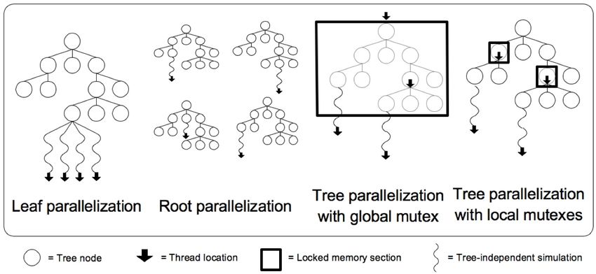
IEEE TRANSACTIONS ON COMPUTATIONAL INTELLIGENCE AND AI IN GAMES, VOL. 4, NO. 1, MARCH 2012                                           3

                                                                   2     BACKGROUND
4 Variations                                                       This section outlines the background theory that led
  4.1 Flat UCB                                                     to the development of MCTS techniques. This includes
  4.2 Bandit Algorithm for Smooth Trees                            decision theory, game theory, and Monte Carlo and
  4.3 Learning in MCTS: TDL; TDMC(λ); BAAL                         bandit-based methods. We emphasise the importance of
  4.4 Single-Player MCTS: FUSE                                     game theory, as this is the domain to which MCTS is
  4.5 Multi-player MCTS: Coalition Reduction                       most applied.
  4.6 Multi-agent MCTS: Ensemble UCT
  4.7 Real-time MCTS
  4.8 Nondeterministic MCTS: Determinization; HOP;                 2.1     Decision Theory
      Sparse UCT; ISUCT; Multiple MCTS; UCT+; MCαβ ;               Decision theory combines probability theory with utility
      MCCFR; Modelling; Simultaneous Moves                         theory to provide a formal and complete framework for
  4.9 Recursive Approaches: Reflexive MC; Nested MC;               decisions made under uncertainty [178, Ch.13].4 Prob-
      NRPA; Meta-MCTS; HGSTS                                       lems whose utility is defined by sequences of decisions
  4.10 Sample-Based Planners: FSSS; TAG; RRTs;                     were pursued in operations research and the study of
      UNLEO; UCTSAT; ρUCT; MRW; MHSP                               Markov decision processes.

5 Tree Policy Enhancements                                         2.1.1    Markov Decision Processes (MDPs)
  5.1 Bandit-Based: UCB1-Tuned; Bayesian UCT; EXP3;
                                                                   A Markov decision process (MDP) models sequential de-
      HOOT; Other
                                                                   cision problems in fully observable environments using
  5.2 Selection: FPU; Decisive Moves; Move Groups;
                                                                   four components [178, Ch.17]:
      Transpositions; Progressive Bias; Opening Books;
      MCPG; Search Seeding; Parameter Tuning;                         • S: A set of states, with s0 being the initial state.

      History Heuristic; Progressive History                          • A: A set of actions.
                                                                                  0
  5.3 AMAF: Permutation; α-AMAF Some-First; Cutoff;                   • T (s, a, s ): A transition model that determines the

      RAVE; Killer RAVE; RAVE-max; PoolRAVE                             probability of reaching state s0 if action a is applied
  5.4 Game-Theoretic: MCTS-Solver; MC-PNS;                              to state s.
      Score Bounded MCTS                                              • R(s): A reward function.

  5.5 Pruning: Absolute; Relative; Domain Knowledge                Overall decisions are modelled as sequences of (state,
  5.6 Expansion                                                    action) pairs, in which each next state s0 is decided by
                                                                   a probability distribution which depends on the current
6 Other Enhancements                                               state s and the chosen action a. A policy is a mapping
  6.1 Simulation: Rule-Based; Contextual; Fill the Board;          from states to actions, specifying which action will be
      Learning; MAST; PAST; FAST; History Heuristics;              chosen from each state in S. The aim is to find the policy
      Evaluation; Balancing; Last Good Reply; Patterns             π that yields the highest expected reward.
  6.2 Backpropagation: Weighting; Score Bonus; Decay;
      Transposition Table Updates                                  2.1.2    Partially Observable Markov Decision Processes
  6.3 Parallelisation: Leaf; Root; Tree; UCT-Treesplit;            If each state is not fully observable, then a Partially
      Threading and Synchronisation                                Observable Markov Decision Process (POMDP) model must
  6.4 Considerations: Consistency; Parameterisation;               be used instead. This is a more complex formulation and
      Comparing Enhancements                                       requires the addition of:
                                                                      • O(s, o): An observation model that specifies the
7 Applications
                                                                        probability of perceiving observation o in state s.
  7.1 Go: Evaluation; Agents; Approaches; Domain
      Knowledge; Variants; Future Work                             The many MDP and POMDP approaches are beyond the
  7.2 Connection Games                                             scope of this review, but in all cases the optimal policy π
  7.3 Other Combinatorial Games                                    is deterministic, in that each state is mapped to a single
  7.4 Single-Player Games                                          action rather than a probability distribution over actions.
  7.5 General Game Playing
  7.6 Real-time Games                                              2.2     Game Theory
  7.7 Nondeterministic Games
  7.8 Non-Game: Optimisation; Satisfaction;                        Game theory extends decision theory to situations in
      Scheduling; Planning; PCG                                    which multiple agents interact. A game can be defined
                                                                   as a set of established rules that allows the interaction
8 Summary                                                          of one5 or more players to produce specified outcomes.
     Impact; Strengths; Weaknesses; Research Directions
                                                                     4. We cite Russell and Norvig [178] as a standard AI reference, to
                                                                   reduce the number of non-MCTS references.
9 Conclusion                                                         5. Single-player games constitute solitaire puzzles.
IEEE TRANSACTIONS ON COMPUTATIONAL INTELLIGENCE AND AI IN GAMES, VOL. 4, NO. 1, MARCH 2012                                    4

   A game may be described by the following compo-                 2.2.2    AI in Real Games
nents:                                                             Real-world games typically involve a delayed reward
   • S: The set of states, where s0 is the initial state.          structure in which only those rewards achieved in the
   • ST ⊆ S: The set of terminal states.                           terminal states of the game accurately describe how well
   • n ∈ N: The number of players.                                 each player is performing. Games are therefore typically
   • A: The set of actions.                                        modelled as trees of decisions as follows:
   • f : S × A → S: The state transition function.
                                                                      • Minimax attempts to minimise the opponent’s max-
                  k
   • R : S → R : The utility function.
                                                                        imum reward at each state, and is the tradi-
   • ρ : S → (0, 1, . . . , n): Player about to act in each
                                                                        tional search approach for two-player combinatorial
     state.                                                             games. The search is typically stopped prematurely
   Each game starts in state s0 and progresses over time                and a value function used to estimate the outcome of
t = 1, 2, . . . until some terminal state is reached. Each              the game, and the α-β heuristic is typically used to
player ki takes an action (i.e. makes a move) that leads,               prune the tree. The maxn algorithm is the analogue
via f , to the next state st+1 . Each player receives a                 of minimax for non-zero-sum games and/or games
reward (defined by the utility function R) that assigns                 with more than two players.
a value to their performance. These values may be                     • Expectimax generalises minimax to stochastic games
arbitrary (e.g. positive values for numbers of points                   in which the transitions from state to state are prob-
accumulated or monetary gains, negative values for costs                abilistic. The value of a chance node is the sum of its
incurred) but in many games it is typical to assign non-                children weighted by their probabilities, otherwise
terminal states a reward of 0 and terminal states a value               the search is identical to maxn . Pruning strategies
of +1, 0 or −1 (or +1, + 21 and 0) for a win, draw or                   are harder due to the effect of chance nodes.
loss, respectively. These are the game-theoretic values of            • Miximax is similar to single-player expectimax and
a terminal state.                                                       is used primarily in games of imperfect information.
   Each player’s strategy (policy) determines the probabil-             It uses a predefined opponent strategy to treat op-
ity of selecting action a given state s. The combination of             ponent decision nodes as chance nodes.
players’ strategies forms a Nash equilibrium if no player
can benefit by unilaterally switching strategies [178,
Ch.17]. Such an equilibrium always exists, but comput-             2.3     Monte Carlo Methods
ing it for real games is generally intractable.                    Monte Carlo methods have their roots in statistical
2.2.1 Combinatorial Games                                          physics where they have been used to obtain approxima-
                                                                   tions to intractable integrals, and have since been used
Games are classified by the following properties:
                                                                   in a wide array of domains including games research.
   • Zero-sum: Whether the reward to all players sums
                                                                      Abramson [1] demonstrated that this sampling might
     to zero (in the two-player case, whether players are          be useful to approximate the game-theoretic value of
     in strict competition with each other).                       a move. Adopting the notation used by Gelly and Sil-
   • Information: Whether the state of the game is fully
                                                                   ver [94], the Q-value of an action is simply the expected
     or partially observable to the players.                       reward of that action:
   • Determinism: Whether chance factors play a part
                                                                                                       N (s)
     (also known as completeness, i.e. uncertainty over                                          1     X
     rewards).                                                                    Q(s, a) =                  Ii (s, a)zi
                                                                                              N (s, a) i=1
   • Sequential: Whether actions are applied sequentially
     or simultaneously.                                            where N (s, a) is the number of times action a has been
   • Discrete: Whether actions are discrete or applied in          selected from state s, N (s) is the number of times a game
     real-time.                                                    has been played out through state s, zi is the result of
  Games with two players that are zero-sum, perfect                the ith simulation played out from s, and Ii (s, a) is 1 if
information, deterministic, discrete and sequential are            action a was selected from state s on the ith play-out
described as combinatorial games. These include games              from state s or 0 otherwise.
such as Go, Chess and Tic Tac Toe, as well as many                    Monte Carlo approaches in which the actions of a
others. Solitaire puzzles may also be described as com-            given state are uniformly sampled are described as flat
binatorial games played between the puzzle designer                Monte Carlo. The power of flat Monte Carlo is demon-
and the puzzle solver, although games with more than               strated by Ginsberg [97] and Sheppard [199], who use
two players are not considered combinatorial due to the            such approaches to achieve world champion level play
social aspect of coalitions that may arise during play.            in Bridge and Scrabble respectively. However it is simple
Combinatorial games make excellent test beds for AI                to construct degenerate cases in which flat Monte Carlo
experiments as they are controlled environments defined            fails, as it does not allow for an opponent model [29].
by simple rules, but which typically exhibit deep and                 Althöfer describes the laziness of flat Monte Carlo in
complex play that can present significant research chal-           non-tight situations [5]. He also describes unexpected
lenges, as amply demonstrated by Go.                               basin behaviour that can occur [6], which might be used
IEEE TRANSACTIONS ON COMPUTATIONAL INTELLIGENCE AND AI IN GAMES, VOL. 4, NO. 1, MARCH 2012                                    5

to help find the optimal UCT search parameters for a               Agrawal [2] introduced policies where the index could
given problem.                                                     be expressed as a simple function of the total reward
   It is possible to improve the reliability of game-              obtained so far by the bandit. Auer et al. [13] subse-
theoretic estimates by biasing action selection based on           quently proposed a variant of Agrawal’s index-based
past experience. Using the estimates gathered so far, it           policy that has a finite-time regret logarithmically bound
is sensible to bias move selection towards those moves             for arbitrary reward distributions with bounded support.
that have a higher intermediate reward.                            One of these variants, UCB1, is introduced next.

                                                                   2.4.2 Upper Confidence Bounds (UCB)
2.4   Bandit-Based Methods
                                                                   For bandit problems, it is useful to know the upper con-
Bandit problems are a well-known class of sequential de-           fidence bound (UCB) that any given arm will be optimal.
cision problems, in which one needs to choose amongst              The simplest UCB policy proposed by Auer et al. [13] is
K actions (e.g. the K arms of a multi-armed bandit slot            called UCB1, which has an expected logarithmic growth
machine) in order to maximise the cumulative reward                of regret uniformly over n (not just asymptotically)
by consistently taking the optimal action. The choice of           without any prior knowledge regarding the reward dis-
action is difficult as the underlying reward distributions         tributions (which have to have their support in [0, 1]).
are unknown, and potential rewards must be estimated               The policy dictates to play arm j that maximises:
based on past observations. This leads to the exploitation-                                        s
exploration dilemma: one needs to balance the exploitation                                            2 ln n
of the action currently believed to be optimal with the                             UCB1 = X j +
                                                                                                        nj
exploration of other actions that currently appear sub-
optimal but may turn out to be superior in the long run.           where X j is the average reward from arm j, nj is the
   A K-armed bandit is defined by random variables                 number of times arm j was played and n is the overall
Xi,n for 1 ≤ i ≤ K and n ≥ 1, where i indicates the arm            number of plays so far. The reward term X j encourages
of the bandit [13], [119], [120]. Successive plays of bandit       the exploitation
                                                                                 q of higher-reward choices, while the right
i yield Xi,1 , Xi,2 , . . . which are independently and iden-      hand term        2 ln n
                                                                                           encourages the exploration of less-
                                                                                      nj
tically distributed according to an unknown law with
                                                                   visited choices. The exploration term is related to the
unknown expectation µi . The K-armed bandit problem
                                                                   size of the one-sided confidence interval for the average
may be approached using a policy that determines which
                                                                   reward within which the true expected reward falls with
bandit to play, based on past rewards.
                                                                   overwhelming probability [13, p 237].
2.4.1 Regret
The policy should aim to minimise the player’s regret,             3     M ONTE C ARLO T REE S EARCH
which is defined after n plays as:                                 This section introduces the family of algorithms known
                                                                   as Monte Carlo Tree Search (MCTS). MCTS rests on two
                                  K
                                  X                                fundamental concepts: that the true value of an action
                RN = µ? n − µj          E[Tj (n)]
                                                                   may be approximated using random simulation; and that
                                  j=1
                                                                   these values may be used efficiently to adjust the policy
where µ? is the best possible expected reward and                  towards a best-first strategy. The algorithm progressively
E[Tj (n)] denotes the expected number of plays for arm             builds a partial game tree, guided by the results of previ-
j in the first n trials. In other words, the regret is             ous exploration of that tree. The tree is used to estimate
the expected loss due to not playing the best bandit.              the values of moves, with these estimates (particularly
It is important to highlight the necessity of attaching            those for the most promising moves) becoming more
non-zero probabilities to all arms at all times, in order          accurate as the tree is built.
to ensure that the optimal arm is not missed due to
temporarily promising rewards from a sub-optimal arm.
                                                                   3.1   Algorithm
It is thus important to place an upper confidence bound
on the rewards observed so far that ensures this.                  The basic algorithm involves iteratively building a search
   In a seminal paper, Lai and Robbins [124] showed                tree until some predefined computational budget – typi-
there exists no policy with a regret that grows slower             cally a time, memory or iteration constraint – is reached,
than O(ln n) for a large class of reward distribu-                 at which point the search is halted and the best-
tions. A policy is subsequently deemed to resolve the              performing root action returned. Each node in the search
exploration-exploitation problem if the growth of regret           tree represents a state of the domain, and directed links
is within a constant factor of this rate. The policies pro-        to child nodes represent actions leading to subsequent
posed by Lai and Robbins made use of upper confidence              states.
indices, which allow the policy to estimate the expected              Four steps are applied per search iteration [52]:
reward of a specific bandit once its index is computed.              1) Selection: Starting at the root node, a child selection
However, these indices were difficult to compute and                    policy is recursively applied to descend through
IEEE TRANSACTIONS ON COMPUTATIONAL INTELLIGENCE AND AI IN GAMES, VOL. 4, NO. 1, MARCH 2012                                            6

              Selection                    Expansion                     Simulation                 Backpropagation

                          Tree                                              Default
                         Policy                                             Policy

Fig. 2. One iteration of the general MCTS approach.

Algorithm 1 General MCTS approach.                                 rithm 1.6 Here v0 is the root node corresponding to state
  function M CTS S EARCH(s0 )                                      s0 , vl is the last node reached during the tree policy
     create root node v0 with state s0                             stage and corresponds to state sl , and ∆ is the reward
     while within computational budget do                          for the terminal state reached by running the default
         vl ← T REE P OLICY(v0 )                                   policy from state sl . The result of the overall search
         ∆ ← D EFAULT P OLICY(s(vl ))                              a(B EST C HILD(v0 )) is the action a that leads to the best
         B ACKUP(vl , ∆)                                           child of the root node v0 , where the exact definition of
     return a(B EST C HILD(v0 ))                                   “best” is defined by the implementation.
                                                                      Note that alternative interpretations of the term “sim-
                                                                   ulation” exist in the literature. Some authors take it
                                                                   to mean the complete sequence of actions chosen per
    the tree until the most urgent expandable node is              iteration during both the tree and default policies (see for
    reached. A node is expandable if it represents a non-          example [93], [204], [94]) while most take it to mean the
    terminal state and has unvisited (i.e. unexpanded)             sequence of actions chosen using the default policy only.
    children.                                                      In this paper we shall understand the terms playout and
 2) Expansion: One (or more) child nodes are added to              simulation to mean “playing out the task to completion
    expand the tree, according to the available actions.           according to the default policy”, i.e. the sequence of
 3) Simulation: A simulation is run from the new node(s)           actions chosen after the tree policy steps of selection and
    according to the default policy to produce an out-             expansion have been completed.
    come.                                                             Figure 2 shows one iteration of the basic MCTS al-
 4) Backpropagation: The simulation result is “backed              gorithm. Starting at the root node7 t0 , child nodes are
    up” (i.e. backpropagated) through the selected                 recursively selected according to some utility function
    nodes to update their statistics.                              until a node tn is reached that either describes a terminal
These may be grouped into two distinct policies:                   state or is not fully expanded (note that this is not
                                                                   necessarily a leaf node of the tree). An unvisited action
 1) Tree Policy: Select or create a leaf node from the             a from this state s is selected and a new leaf node tl is
    nodes already contained within the search tree (se-            added to the tree, which describes the state s0 reached
    lection and expansion).                                        from applying action a to state s. This completes the tree
 2) Default Policy: Play out the domain from a given               policy component for this iteration.
    non-terminal state to produce a value estimate (sim-              A simulation is then run from the newly expanded
    ulation).                                                      leaf node tl to produce a reward value ∆, which is then
The backpropagation step does not use a policy itself,
but updates node statistics that inform future tree policy           6. The simulation and expansion steps are often described and/or
                                                                   implemented in the reverse order in practice [52], [67].
decisions.
                                                                     7. Each node contains statistics describing at least a reward value
  These steps are summarised in pseudocode in Algo-                and number of visits.
IEEE TRANSACTIONS ON COMPUTATIONAL INTELLIGENCE AND AI IN GAMES, VOL. 4, NO. 1, MARCH 2012                                             7

backpropagated up the sequence of nodes selected for               This may be achieved by reducing the estimation error
this iteration to update the node statistics; each node’s          of the nodes’ values as quickly as possible. In order
visit count is incremented and its average reward or               to do so, the algorithm must balance exploitation of
Q value updated according to ∆. The reward value ∆                 the currently most promising action with exploration of
may be a discrete (win/draw/loss) result or continuous             alternatives which may later turn out to be superior.
reward value for simpler domains, or a vector of reward            This exploitation-exploration dilemma can be captured
values relative to each agent p for more complex multi-            by multi-armed bandit problems (2.4), and UCB1 [13] is
agent domains.                                                     an obvious choice for node selection. 8
   As soon as the search is interrupted or the computa-               Table 1 summarises the milestones that led to the
tion budget is reached, the search terminates and an ac-           conception and popularisation of MCTS. It is interesting
tion a of the root node t0 is selected by some mechanism.          to note that the development of MCTS is the coming
Schadd [188] describes four criteria for selecting the             together of numerous different results in related fields
winning action, based on the work of Chaslot et al [60]:           of research in AI.
  1) Max child: Select the root child with the highest
     reward.                                                       3.3   Upper Confidence Bounds for Trees (UCT)
  2) Robust child: Select the most visited root child.
                                                                   This section describes the most popular algorithm in the
  3) Max-Robust child: Select the root child with both the
                                                                   MCTS family, the Upper Confidence Bound for Trees (UCT)
     highest visit count and the highest reward. If none
                                                                   algorithm. We provide a detailed description of the
     exist, then continue searching until an acceptable
                                                                   algorithm, and briefly outline the proof of convergence.
     visit count is achieved [70].
  4) Secure child: Select the child which maximises a
     lower confidence bound.                                       3.3.1 The UCT algorithm
                                                                   The goal of MCTS is to approximate the (true) game-
                                                                   theoretic value of the actions that may be taken from
3.2   Development                                                  the current state (3.1). This is achieved by iteratively
Monte Carlo methods have been used extensively in                  building a partial search tree, as illustrated in Figure 2.
games with randomness and partial observability [70]               How the tree is built depends on how nodes in the tree
but they may be applied equally to deterministic games             are selected. The success of MCTS, especially in Go, is
of perfect information. Following a large number of                primarily due to this tree policy. In particular, Kocsis
simulated games, starting at the current state and played          and Szepesvári [119], [120] proposed the use of UCB1
until the end of the game, the initial move with the               (2.4.2) as tree policy. In treating the choice of child node
highest win-rate is selected to advance the game. In the           as a multi-armed bandit problem, the value of a child
majority of cases, actions were sampled uniformly at               node is the expected reward approximated by the Monte
random (or with some game-specific heuristic bias) with            Carlo simulations, and hence these rewards correspond
no game-theoretic guarantees [119]. In other words, even           to random variables with unknown distributions.
if the iterative process is executed for an extended period           UCB1 has some promising properties: it is very simple
of time, the move selected in the end may not be optimal           and efficient and guaranteed to be within a constant
[120].                                                             factor of the best possible bound on the growth of
   Despite the lack of game-theoretic guarantees, the ac-          regret. It is thus a promising candidate to address the
curacy of the Monte Carlo simulations may often be im-             exploration-exploitation dilemma in MCTS: every time a
proved by selecting actions according to the cumulative            node (action) is to be selected within the existing tree, the
reward of the game episodes they were part of. This may            choice may be modelled as an independent multi-armed
be achieved by keeping track of the states visited in a            bandit problem. A child node j is selected to maximise:
tree. In 2006 Coulom [70] proposed a novel approach that                                                s
combined Monte Carlo evaluations with tree search. His                                                    2 ln n
                                                                                    U CT = X j + 2Cp
proposed algorithm iteratively runs random simulations                                                      nj
from the current state to the end of the game: nodes
close to the root are added to an incrementally growing            where n is the number of times the current (parent) node
tree, revealing structural information from the random             has been visited, nj the number of times child j has
sampling episodes. In particular, nodes in the tree are            been visited and Cp > 0 is a constant. If more than one
selected according to the estimated probability that they          child node has the same maximal value, the tie is usually
are better than the current best move.                             broken randomly [120]. The values of Xi,t and thus of
   The breakthrough for MCTS also came in 2006 and                 X j are understood to be within [0, 1] (this holds true
is primarily due to the selectivity mechanism proposed             for both the UCB1 and the UCT proofs). It is generally
by Kocsis and Szepesvári, whose aim was to design a               understood that nj = 0 yields a UCT value of ∞, so that
Monte Carlo search algorithm that had a small error
                                                                     8. Coulom [70] points out that the Boltzmann distribution often used
probability if stopped prematurely and that converged to           in n-armed bandit problems is not suitable as a selection mechanism,
the game-theoretic optimum given sufficient time [120].            as the underlying reward distributions in the tree are non-stationary.
IEEE TRANSACTIONS ON COMPUTATIONAL INTELLIGENCE AND AI IN GAMES, VOL. 4, NO. 1, MARCH 2012                                                8

    1990    Abramson demonstrates that Monte Carlo simulations can be used to evaluate value of state [1].
    1993    Brügmann [31] applies Monte Carlo methods to the field of computer Go.
    1998    Ginsberg’s GIB program competes with expert Bridge players.
    1998    MAVEN defeats the world scrabble champion [199].
    2002    Auer et al. [13] propose UCB1 for multi-armed bandit, laying the theoretical foundation for UCT.
    2006    Coulom [70] describes Monte Carlo evaluations for tree-based search, coining the term Monte Carlo tree search.
    2006    Kocsis and Szepesvari [119] associate UCB with tree-based search to give the UCT algorithm.
    2006    Gelly et al. [96] apply UCT to computer Go with remarkable success, with their program M O G O.
    2006    Chaslot et al. describe MCTS as a broader framework for game AI [52] and general domains [54].
    2007    C ADIA P LAYER becomes world champion General Game Player [83].
    2008    M O G O achieves dan (master) level at 9 × 9 Go [128].
    2009    F UEGO beats top human professional at 9 × 9 Go [81].
    2009    M O H EX becomes world champion Hex player [7].

                                                           TABLE 1
                              Timeline of events leading to the widespread popularity of MCTS.

previously unvisited children are assigned the largest                 part of a playout from the root, its values are updated.
possible value, to ensure that all children of a node are              Once some computational budget has been reached, the
considered at least once before any child is expanded                  algorithm terminates and returns the best move found,
further. This results in a powerful form of iterated local             corresponding to the child of the root with the highest
search.                                                                visit count.
   There is an essential balance between the first (ex-                   Algorithm 2 shows the UCT algorithm in pseudocode.
ploitation) and second (exploration) terms of the UCB                  This code is a summary of UCT descriptions from several
equation. As each node is visited, the denominator of the              sources, notably [94], but adapted to remove the two-
exploration term increases, which decreases its contribu-              player, zero-sum and turn order constraints typically
tion. On the other hand, if another child of the parent                found in the existing literature.
node is visited, the numerator increases and hence the                    Each node v has four pieces of data associated with
exploration values of unvisited siblings increase. The                 it: the associated state s(v), the incoming action a(v), the
exploration term ensures that each child has a non-                    total simulation reward Q(v) (a vector of real values),
zero probability of selection, which is essential given                and the visit count N (v) (a nonnegative integer). Instead
the random nature of the playouts. This also imparts an                of storing s(v) for each node, it is often more efficient in
inherent restart property to the algorithm, as even low-               terms of memory usage to recalculate it as T REE P OLICY
reward children are guaranteed to be chosen eventually                 descends the tree. The term ∆(v, p) denotes the compo-
(given sufficient time), and hence different lines of play             nent of the reward vector ∆ associated with the current
explored.                                                              player p at node v.
   The constant in the exploration term Cp can be ad-                     The return value of the overall search in this case is
justed to lower or increase the √ amount of exploration                a(B EST C HILD(v0 , 0)) which will give the action a that
performed. The value Cp = 1/ 2 was shown by Kocsis                     leads to the child with the highest reward,10 since the
and Szepesvári [120] to satisfy the Hoeffding ineqality               exploration parameter c is set to 0 for this final call on
with rewards in the range [0, 1]. With rewards outside                 the root node v0 . The algorithm could instead return
this range, a different value of Cp may be needed and                  the action that leads to the most visited child; these
also certain enhancements9 work better with a different                two options will usually – but not always! – describe
value for Cp (7.1.3).                                                  the same action. This potential discrepancy is addressed
   The rest of the algorithm proceeds as described in                  in the Go program E RICA by continuing the search if
Section 3.1: if the node selected by UCB descent has                   the most visited root action is not also the one with
children that are not yet part of the tree, one of those is            the highest reward. This improved E RICA’s winning rate
chosen randomly and added to the tree. The default pol-                against GNU G O from 47% to 55% [107].
icy is then used until a terminal state has been reached.                 Algorithm 3 shows an alternative and more efficient
In the simplest case, this default policy is uniformly                 backup method for two-player, zero-sum games with al-
random. The value ∆ of the terminal state sT is then                   ternating moves, that is typically found in the literature.
backpropagated to all nodes visited during this iteration,             This is analogous to the negamax variant of minimax
from the newly added node to the root.                                 search, in which scalar reward values are negated at each
   Each node holds two values, the number N (v) of times               level in the tree to obtain the other player’s reward. Note
it has been visited and a value Q(v) that corresponds                  that while ∆ is treated as a vector of rewards with an
to the total reward of all playouts that passed through                entry for each agent in Algorithm 2,11 it is a single scalar
this state (so that Q(v)/N (v) is an approximation of                  value representing the reward to the agent running the
the node’s game-theoretic value). Every time a node is
                                                                         10. The max child in Schadd’s [188] terminology.
  9. Such as RAVE (5.3.5).                                               11. ∆(v, p) denotes the reward for p the player to move at node v.
IEEE TRANSACTIONS ON COMPUTATIONAL INTELLIGENCE AND AI IN GAMES, VOL. 4, NO. 1, MARCH 2012 9
Algorithm 2 The UCT algorithm. 3.3.2 Convergence to Minimax
function U CT S EARCH(s0 ) The key contributions of Kocsis and Szepesvári [119],
create root node v0 with state s0 [120] were to show that the bound on the regret of UCB1
while within computational budget do still holds in the case of non-stationary reward distribu-
vl ← T REE P OLICY(v0 ) tions, and to empirically demonstrate the workings of
∆ ← D EFAULT P OLICY(s(vl )) MCTS with UCT on a variety of domains. Kocsis and
B ACKUP(vl , ∆) Szepesvári then show that the failure probability at the
return a(B EST C HILD(v0 , 0)) root of the tree (i.e. the probability of selecting a subop-
timal action) converges to zero at a polynomial rate as
function T REE P OLICY(v) the number of games simulated grows to infinity. This
while v is nonterminal do proof implies that, given enough time (and memory),
if v not fully expanded then UCT allows MCTS to converge to the minimax tree and
return E XPAND(v) is thus optimal.
else
v ← B EST C HILD(v, Cp) 3.4 Characteristics
return v This section describes some of the characteristics that
make MCTS a popular choice of algorithm for a variety
function E XPAND(v) of domains, often with notable success.
choose a ∈ untried actions from A(s(v))
add a new child v 0 to v 3.4.1 Aheuristic
with s(v 0 ) = f (s(v), a) One of the most significant benefits of MCTS is the
and a(v 0 ) = a lack of need for domain-specific knowledge, making it
return v 0 readily applicable to any domain that may be modelled
using a tree. Although full-depth minimax is optimal in
function B EST C HILD(v, c) s the game-theoretic sense, the quality of play for depth-
Q(v 0 ) 2 ln N (v) limited minimax depends significantly on the heuristic
return arg max +c
0
v ∈children of v N (v )
0 N (v 0 ) used to evaluate leaf nodes. In games such as Chess,
where reliable heuristics have emerged after decades
of research, minimax performs admirably well. In cases
function D EFAULT P OLICY(s)
such as Go, however, where branching factors are orders
while s is non-terminal do
of magnitude larger and useful heuristics are much
choose a ∈ A(s) uniformly at random
more difficult to formulate, the performance of minimax
s ← f (s, a)
degrades significantly.
return reward for state s Although MCTS can be applied in its absence, sig-
nificant improvements in performance may often be
function B ACKUP(v, ∆) achieved using domain-specific knowledge. All top-
while v is not null do performing MCTS-based Go programs now use game-
N (v) ← N (v) + 1 specific information, often in the form of patterns (6.1.9).
Q(v) ← Q(v) + ∆(v, p) Such knowledge need not be complete as long as it is
v ← parent of v able to bias move selection in a favourable fashion.
There are trade-offs to consider when biasing move
selection using domain-specific knowledge: one of the
advantages of uniform random move selection is speed,
Algorithm 3 UCT backup for two players. allowing one to perform many simulations in a given
function B ACKUP N EGAMAX(v, ∆) time. Domain-specific knowledge usually drastically re-
while v is not null do duces the number of simulations possible, but may also
N (v) ← N (v) + 1 reduce the variance of simulation results. The degree
Q(v) ← Q(v) + ∆ to which game-specific knowledge should be included,
∆ ← −∆ with respect to performance versus generality as well as
v ← parent of v speed trade-offs, is discussed in [77].
3.4.2 Anytime
MCTS backpropagates the outcome of each game im-
mediately (the tree is built using playouts as opposed
search in Algorithm 3. Similarly, the node reward value to stages [119]) which ensures all values are always up-
Q(v) may be treated as a vector of values for each player to-date following every iteration of the algorithm. This
Q(v, p) should circumstances dictate. allows the algorithm to return an action from the root atIEEE TRANSACTIONS ON COMPUTATIONAL INTELLIGENCE AND AI IN GAMES, VOL. 4, NO. 1, MARCH 2012 10
ensures that the true minimax values are known.12 In
this domain, UCT clearly outperforms minimax and the
gap in performance increases with tree depth.
Ramanujan et al. [162] argue that UCT performs
poorly in domains with many trap states (states that lead
to losses within a small number of moves), whereas iter-
ative deepening minimax performs relatively well. Trap
states are common in Chess but relatively uncommon
in Go, which may go some way towards explaining the
algorithms’ relative performance in those games.
3.6 Terminology
The terms MCTS and UCT are used in a variety of
ways in the literature, sometimes inconsistently, poten-
tially leading to confusion regarding the specifics of the
Fig. 3. Asymmetric tree growth [68]. algorithm referred to. For the remainder of this survey,
we adhere to the following meanings:
• Flat Monte Carlo: A Monte Carlo method with
any moment in time; allowing the algorithm to run for
additional iterations often improves the result. uniform move selection and no tree growth.
• Flat UCB: A Monte Carlo method with bandit-based
It is possible to approximate an anytime version of
minimax using iterative deepening. However, the gran- move selection (2.4) but no tree growth.
• MCTS: A Monte Carlo method that builds a tree to
ularity of progress is much coarser as an entire ply is
added to the tree on each iteration. inform its policy online.
• UCT: MCTS with any UCB tree selection policy.
• Plain UCT: MCTS with UCB1 as proposed by Kocsis
3.4.3 Asymmetric
and Szepesvári [119], [120].
The tree selection allows the algorithm to favour more In other words, “plain UCT” refers to the specific algo-
promising nodes (without allowing the selection proba- rithm proposed by Kocsis and Szepesvári, whereas the
bility of the other nodes to converge to zero), leading other terms refer more broadly to families of algorithms.
to an asymmetric tree over time. In other words, the
building of the partial tree is skewed towards more
promising and thus more important regions. Figure 3 4 VARIATIONS
from [68] shows asymmetric tree growth using the BAST Traditional game AI research focusses on zero-sum
variation of MCTS (4.2). games with two players, alternating turns, discrete ac-
The tree shape that emerges can even be used to gain a tion spaces, deterministic state transitions and perfect
better understanding about the game itself. For instance, information. While MCTS has been applied extensively
Williams [231] demonstrates that shape analysis applied to such games, it has also been applied to other domain
to trees generated during UCT search can be used to types such as single-player games and planning prob-
distinguish between playable and unplayable games. lems, multi-player games, real-time games, and games
with uncertainty or simultaneous moves. This section
3.5 Comparison with Other Algorithms describes the ways in which MCTS has been adapted
to these domains, in addition to algorithms that adopt
When faced with a problem, the a priori choice between ideas from MCTS without adhering strictly to its outline.
MCTS and minimax may be difficult. If the game tree
is of nontrivial size and no reliable heuristic exists for
the game of interest, minimax is unsuitable but MCTS 4.1 Flat UCB
is applicable (3.4.1). If domain-specific knowledge is Coquelin and Munos [68] propose flat UCB which effec-
readily available, on the other hand, both algorithms tively treats the leaves of the search tree as a single multi-
may be viable approaches. armed bandit problem. This is distinct from flat Monte
However, as pointed out by Ramanujan et al. [164], Carlo search (2.3) in which the actions for a given state
MCTS approaches to games such as Chess are not as are uniformly sampled and no tree is built. Coquelin
successful as for games such as Go. They consider a and Munos [68] demonstrate that flat UCB retains the
class of synthetic spaces in which UCT significantly adaptivity of standard UCT while improving its regret
outperforms minimax. In particular, the model produces bounds in certain worst cases where UCT is overly
bounded trees where there is exactly one optimal action optimistic.
per state; sub-optimal choices are penalised with a fixed
additive cost. The systematic construction of the tree 12. This is related to P-game trees (7.3).IEEE TRANSACTIONS ON COMPUTATIONAL INTELLIGENCE AND AI IN GAMES, VOL. 4, NO. 1, MARCH 2012 11
4.2 Bandit Algorithm for Smooth Trees (BAST) 4.4 Single-Player MCTS (SP-MCTS)
Coquelin and Munos [68] extend the flat UCB model Schadd et al. [191], [189] introduce a variant of MCTS
to suggest a Bandit Algorithm for Smooth Trees (BAST), for single-player games, called Single-Player Monte Carlo
which uses assumptions on the smoothness of rewards to Tree Search (SP-MCTS), which adds a third term to the
identify and ignore branches that are suboptimal with standard UCB formula that represents the “possible
high confidence. They applied BAST to Lipschitz func- deviation” of the node. This term can be written
tion approximation and showed that when allowed to
r
D
run for infinite time, the only branches that are expanded σ2 + ,
ni
indefinitely are the optimal branches. This is in contrast
to plain UCT, which expands all branches indefinitely. where σ 2 is the variance of the node’s simulation results,
ni is the number of visits to the node, and D is a
constant. The nDi term can be seen as artificially inflating
4.3 Learning in MCTS the standard deviation for infrequently visited nodes, so
that the rewards for such nodes are considered to be
MCTS can be seen as a type of Reinforcement Learning less certain. The other main difference between SP-MCTS
(RL) algorithm, so it is interesting to consider its rela- and plain UCT is the use of a heuristically guided default
tionship with temporal difference learning (arguably the policy for simulations.
canonical RL algorithm). Schadd et al. [191] point to the need for Meta-Search
(a higher-level search method that uses other search
4.3.1 Temporal Difference Learning (TDL) processes to arrive at an answer) in some cases where
SP-MCTS on its own gets caught in local maxima. They
Both temporal difference learning (TDL) and MCTS learn found that periodically restarting the search with a dif-
to take actions based on the values of states, or of state- ferent random seed and storing the best solution over
action pairs. Under certain circumstances the algorithms all runs considerably increased the performance of their
may even be equivalent [201], but TDL algorithms do not SameGame player (7.4).
usually build trees, and the equivalence only holds when
Björnsson and Finnsson [21] discuss the application of
all the state values can be stored directly in a table. MCTS
standard UCT to single-player games. They point out
estimates temporary state values in order to decide the
that averaging simulation results can hide a strong line
next move, whereas TDL learns the long-term value
of play if its siblings are weak, instead favouring regions
of each state that then guides future behaviour. Silver
where all lines of play are of medium strength. To
et al. [202] present an algorithm that combines MCTS
counter this, they suggest tracking maximum simulation
with TDL using the notion of permanent and transient
results at each node in addition to average results; the
memories to distinguish the two types of state value
averages are still used during search.
estimation. TDL can learn heuristic value functions to
Another modification suggested by Björnsson and
inform the tree policy or the simulation (playout) policy.
Finnsson [21] is that when simulation finds a strong line
of play, it is stored in the tree in its entirety. This would
4.3.2 Temporal Difference with Monte Carlo (TDMC(λ)) be detrimental in games of more than one player since
such a strong line would probably rely on the unrealistic
Osaki et al. describe the Temporal Difference with Monte
assumption that the opponent plays weak moves, but for
Carlo (TDMC(λ)) algorithm as “a new method of rein-
single-player games this is not an issue.
forcement learning using winning probability as substi-
tute rewards in non-terminal positions” [157] and report
superior performance over standard TD learning for the 4.4.1 Feature UCT Selection (FUSE)
board game Othello (7.3). Gaudel and Sebag introduce Feature UCT Selection
(FUSE), an adaptation of UCT to the combinatorial op-
timisation problem of feature selection [89]. Here, the
4.3.3 Bandit-Based Active Learner (BAAL)
problem of choosing a subset of the available features is
Rolet et al. [175], [173], [174] propose the Bandit-based cast as a single-player game whose states are all possible
Active Learner (BAAL) method to address the issue of subsets of features and whose actions consist of choosing
small training sets in applications where data is sparse. a feature and adding it to the subset.
The notion of active learning is formalised under bounded To deal with the large branching factor of this game,
resources as a finite horizon reinforcement learning prob- FUSE uses UCB1-Tuned (5.1.1) and RAVE (5.3.5). FUSE
lem with the goal of minimising the generalisation error. also uses a game-specific approximation of the reward
Viewing active learning as a single-player game, the function, and adjusts the probability of choosing the
optimal policy is approximated by a combination of stopping feature during simulation according to the
UCT and billiard algorithms [173]. Progressive widening depth in the tree. Gaudel and Sebag [89] apply FUSE
(5.5.1) is employed to limit the degree of exploration by to three benchmark data sets from the NIPS 2003 FS
UCB1 to give promising empirical results. Challenge competition (7.8.4).IEEE TRANSACTIONS ON COMPUTATIONAL INTELLIGENCE AND AI IN GAMES, VOL. 4, NO. 1, MARCH 2012 12
4.5 Multi-player MCTS (or learned, as in [139]), using multiple agents improves
The central assumption of minimax search (2.2.2) is that playing strength. Marcolino and Matsubara [139] argue
the searching player seeks to maximise their reward that the emergent properties of interactions between
while the opponent seeks to minimise it. In a two-player different agent types lead to increased exploration of the
zero-sum game, this is equivalent to saying that each search space. However, finding the set of agents with
player seeks to maximise their own reward; however, in the correct properties (i.e. those that increase playing
games of more than two players, this equivalence does strength) is computationally intensive.
not necessarily hold.
The simplest way to apply MCTS to multi-player 4.6.1 Ensemble UCT
games is to adopt the maxn idea: each node stores a Fern and Lewis [82] investigate an Ensemble UCT ap-
vector of rewards, and the selection procedure seeks to proach, in which multiple instances of UCT are run
maximise the UCB value calculated using the appropri- independently and their root statistics combined to yield
ate component of the reward vector. Sturtevant [207] the final result. This approach is closely related to root
shows that this variant of UCT converges to an opti- parallelisation (6.3.2) and also to determinization (4.8.1).
mal equilibrium strategy, although this strategy is not Chaslot et al. [59] provide some evidence that, for
precisely the maxn strategy as it may be mixed. Go, Ensemble UCT with n instances of m iterations
Cazenave [40] applies several variants of UCT to the each outperforms plain UCT with mn iterations, i.e.
game of Multi-player Go (7.1.5) and considers the possi- that Ensemble UCT outperforms plain UCT given the
bility of players acting in coalitions. The search itself uses same total number of iterations. However, Fern and
the maxn approach described above, but a rule is added Lewis [82] are not able to reproduce this result on other
to the simulations to avoid playing moves that adversely experimental domains.
affect fellow coalition members, and a different scoring
system is used that counts coalition members’ stones as 4.7 Real-time MCTS
if they were the player’s own. Traditional board games are turn-based, often allowing
There are several ways in which such coalitions can each player considerable time for each move (e.g. several
be handled. In Paranoid UCT, the player considers that minutes for Go). However, real-time games tend to
all other players are in coalition against him. In UCT progress constantly even if the player attempts no move,
with Alliances, the coalitions are provided explicitly to so it is vital for an agent to act quickly. The largest class
the algorithm. In Confident UCT, independent searches of real-time games are video games, which – in addition
are conducted for each possible coalition of the searching to the real-time element – are usually also characterised
player with one other player, and the move chosen by uncertainty (4.8), massive branching factors, simulta-
according to whichever of these coalitions appears most neous moves (4.8.10) and open-endedness. Developing
favourable. Cazenave [40] finds that Confident UCT strong artificial players for such games is thus particu-
performs worse than Paranoid UCT in general, but the larly challenging and so far has been limited in success.
performance of the former is better when the algorithms Simulation-based (anytime) algorithms such as MCTS
of the other players (i.e. whether they themselves use are well suited to domains in which time per move is
Confident UCT) are taken into account. Nijssen and strictly limited. Furthermore, the asymmetry of the trees
Winands [155] describe the Multi-Player Monte-Carlo Tree produced by MCTS may allow a better exploration of
Search Solver (MP-MCTS-Solver) version of their MCTS the state space in the time available. Indeed, MCTS has
Solver enhancement (5.4.1). been applied to a diverse range of real-time games of
increasing complexity, ranging from Tron and Ms. Pac-
4.5.1 Coalition Reduction Man to a variety of real-time strategy games akin to
Winands and Nijssen describe the coalition reduction Starcraft. In order to make the complexity of real-time
method [156] for games such as Scotland Yard (7.7) in video games tractable, approximations may be used to
which multiple cooperative opponents can be reduced to increase the efficiency of the forward model.
a single effective opponent. Note that rewards for those
opponents who are not the root of the search must be 4.8 Nondeterministic MCTS
biased to stop them getting lazy [156].
Traditional game AI research also typically focusses on
deterministic games with perfect information, i.e. games
4.6 Multi-agent MCTS without chance events in which the state of the game
Marcolino and Matsubara [139] describe the simulation is fully observable to all players (2.2). We now consider
phase of UCT as a single agent playing against itself, and games with stochasticity (chance events) and/or imperfect
instead consider the effect of having multiple agents (i.e. information (partial observability of states).
multiple simulation policies). Specifically, the different Opponent modelling (i.e. determining the opponent’s
agents in this case are obtained by assigning different policy) is much more important in games of imperfect
priorities to the heuristics used in Go program F UEGO’s information than games of perfect information, as the
simulations [81]. If the right subset of agents is chosen opponent’s policy generally depends on their hiddenYou can also read