Calculation of Mohr-Coulomb Parameters for Rocks of Doha, Qatar
←
→
Page content transcription
If your browser does not render page correctly, please read the page content below
Calculation of Mohr-Coulomb Parameters for Rocks of Doha, Qatar Hrvoje Vučemilović ( hvucemilovic@gfos.hr ) University of Osijek https://orcid.org/0000-0002-1366-5373 Research Article Keywords: Qatar, Doha, Rocks, Calculation, Mohr-Coulomb, Hoek-Brown DOI: https://doi.org/10.21203/rs.3.rs-559195/v1 License: This work is licensed under a Creative Commons Attribution 4.0 International License. Read Full License
TECHNICAL NOTE

                                  Calculation of Mohr-Coulomb Parameters for Rocks of Doha, Qatar

    Hrvoje Vučemilović 1,2

    1 - Qatar Trading and Contracting Group

    2 - University of J.J. Strossmayer in Osijek, Croatia, Faculty of civil engineering and architecture

    Author ORCID: 0000-0002-1366-5373, hvucemilovic@gfos.hr

Abstract

Among practitioners, designers and researchers, modern-day geotechnical software packages still predominantly use Mohr-Coulomb

(MC) input modelling parameters, despite the immense computing power of today’s software and hardware components. The same

particularly applies to this field of work in the state of Qatar. The goal of this technical note is to demonstrate the most appropriate

derivation method for Mohr-Coulomb parameters, by proving that this must ensue by first obtaining or estimating proper Hoek-Brown

parameters, followed by appropriate method for conversion. Only such an approach can remove uncertainty and high variability of

results in geotechnical estimations and design inputs.

Keywords: Qatar; Doha; Rocks; Calculation; Mohr-Coulomb; Hoek-Brown

1           Introduction

This technical note is based on the data and results from Vucemilovic et al. (2021), previous works and publications of Evert Hoek and

his co-researchers, and on previous publications on Qatari rock masses that have dealt with providing Mohr-Coulomb parameters.

Previous works on this particular subject thus include Fourniadis (2010), Karagkounis et al. (2016) and Vucemilovic et al. (2021). Their

results are summed up in table 1, and include cohesion and friction angle values for three geological members/ layers of rock masses of

Doha Qatar, which are Simsima Limestone (SL), Midra Shale (MSH) and Rus Formation (RUS).

In his paper Fourniadis (2010) cites Hoek et al. (1995) as the conversion method, whereas Karagkounis et al. (2016) cite Hoek et al.

(2002) along with Carter et al. (2008) and Latapie and Lochaden (2016). Karagkounis et al. (2016) also mention “adequate maximum

confining stresses” in relation to their findings but it is unclear if triaxial tests were used or not, however no such result data were

presented. Neither of two (groups of) authors gave any further specifics in terms of equations or data except the final value ranges. As

we can see in table 1, data reported by Vucemilovic et al. (2021) are significantly different than those for other two authors, and the

authors indicated that these results were obtained by improper conduction of triaxial tests, where confinement σ3 loads were

insufficiently large, except by chance, for RUS member. Results from final three rows of the table 1 are calculated and elaborated

further down the contents of this paper.
Table 1. Mohr-Coulomb data from previous authors on Qatari rock masses and this technical note
Author Layer/Member c [MPa] φ [deg]
Fourniadis (2010) SL 0.14 – 0.65 21 – 32
Karagkounis et al. (2016) SL 0.03 – 0.44 21 – 47
MSH 0.04 – 0.35 33 – 46
RUS 0.03 – 0.20 30 – 48
Vucemilovic et al. (2021) SL 0.10 – 3.00 53 – 79
MSH 0.50 – 3.20 55 - 73
RUS 0.10 – 2.60 42 - 79
This technical note SL 1.12 24.57
MSH 0.82 25.39
RUS 0.69 28.94
In their paper, Vucemilovic et al. (2021) have stated that rock masses of Doha, Qatar, should be treated as applicable for Hoek-Brown
(HB) criterion, since they are sufficiently strong and above the transition zone towards soils according to classification proposals by
Carter et al. (2008) and Carvalho et al. (2007). The only exception is the RUS member which can be considered as falling under the
top region of this zone, but even so, the Carvalho et al. (2007) transitional parameters are hardly changed from Hoek et al. (2002)
outset parameters s, a, and mb (Vucemilovic et al. 2021). The table 2 shows the intact rock parameters obtained by Vucemilovic et al.
(2021), where the authors, deprived of possibility to obtain HB parameters for SL and MSH geological members, resorted to auxiliary
solutions from other authors (Arshadnejad and Nick 2016 and Cai 2010). The addition to the table as it appeared in Vucemilovic et al.
(2021) is the “This tech. note” column.
Table 2. Summary of the derived mi and related values from equations by several authorsa (Vucemilovic et al. 2021) with added adopted values of mi
HOEK and HOEK et al. 2002 ARSHADNEJAD CAI This CARVALHO et al. 2007
tech.
BROWN 1980a and NICK 2016 2009 note
n σ ci mi a s mb mb mi R index Adopted fT(UCS) s* a* mb *
(UCS/ values of
mi
BTS)
SL 123 12.54 179.2 0.51 0.00127 21.02 0.774 6.60 7.75 6.50
MSH 33 14.41 78.0 0.51 0.00142 9.48 0.843 6.94 8.36 7.00
RUS 57 18.15 8.23 0.50 0.00345 1.33 1.457 9.01 12.51 8.50 0.00213 0.00557 0.501 1.35
a italic = incoherent results; bold = good agreement; bold = adopted valuesFigure 1. Inappropriate devices (left) and methods (right) for execution and elaboration of triaxial tests reported by Vucemilovic et al. (2021)
The triaxial data reported by Vucemilovic et al. (2021), as all other triaxial data to author’s best knowledge, were obtained with above
shown (figure 1) equipment and method, by local commercial geotechnical laboratories. The figure 1 (left) shows a triaxial apparatus
which is elsewhere in the world used for soft soil (clays) testing. It is capable of reaching a confinement load of maximum 1.7 MPa
which is insufficient for local rock samples and it produces the pressure with water. Figure 1 (right) shows the method of obtaining
MC parameters c and φ. The σ1 – σ3 data pairs are graphically plotted and Mohr circles are drawn from them, however with
insufficiently large confinement load, the tangent gives very steep φ angles. This derivation method is described in ASTM D7012-10
(2010) standard.
2 HB criterion and MC conversion
During the development of the Hoek-Brown criterion, between 1983 and 2002, Hoek (et al.) gave a total of six different methods of
conversion to MC parameters, for equal number of HB criterion major development steps. These methods were laid out in Hoek
(1983), Hoek (1990), Hoek et al. (1992), Hoek et al. (1995), Hoek and Brown (1997) and Hoek et al. (2002). Of these six, only two of
the methods are applicable for the problem at hand, where triaxial data pairs σ 1 and σ3 are available only, as opposed to proposals
where effective stresses are known, e.g. for slope, tunneling and other problems. These are Hoek (1983) and Hoek & Brown (1997)
approaches. The expressions for Hoek (1983) are as follows:
3'
' 2
' ' 1
3 (1)
2 1' 3' m c
n
1
2
1/2
m c
1
' '
(2)
1
2 1' 3'
3
2
i' 90 arcsin '
1 3'
(3)
If equations (1) to (3) are applied to triaxial results for RUS member from Vucemilovic et al. (2021), incoherent results are obtained,
in spite of the fact that the triaxial results yielded a coherent mi parameter result. Only the first five data point results are shown in
table 3, and it is visible in the right-most column that such results are obtained where the argument of the arcsin function, from
equation (3) is larger than unity. Thus, the method cannot give the desired results, since data do not allow it.
Table 3. Sample calculation of MC values from triaxial test results for RUS member, from Hoek (1983) equations (1) to (3)
2τ/
σ3 = X σ1 Y XY X2 Y2 σn τ
(σ1 - σ3)
0.3 9.41 82.99 24.90 0.09 6887.69 1.46 23.81 5.23
0.3 25.00 610.09 183.03 0.09 372209.81 6.25 43.84 3.55
0.65 10.41 95.26 61.92 0.42 9074.01 1.96 24.77 5.08
0.6 15.68 227.41 136.44 0.36 51713.67 3.33 32.07 4.25
0.4 6.88 41.99 16.80 0.16 1763.19 1.04 19.65 6.06
The only other approach which is applicable for MC values to be obtained from principal stresses from triaxial tests is that of Hoek &
Brown (1997). This approach is the reverse of core Hoek-Brown principle where mi constant is calculated from triaxial test results.
Triaxial data pairs are simulated to produce eight data pairs in the range 0 < σ3 < 0.25 UCS. The full details of the procedure are laid
out in Hoek & Brown (1997), Appendix C. Theoretical equations that represent the method, which are an amalgam of Hoek & Brown
(1997) and earlier works, are equations (4) to (16). In this approach one must know, or correctly assume the mi value. In our case, we
must make the best assumption for the intact rock constant mi values based on the results from table 2, which is not a straightforward
task, and there are no guarantees that the chosen values are the optimal. The chosen values are shown in table 2 under “this tech. note”
column, and are estimated from obtained value of mi for RUS, Arshadnejad & Nick (2016) values and on Cai (2009) R-index values
and how they relate to each other for three geological members. It is also visible that the values increase with depth.
B
' tm
A ci (4)
ci
' tm
log log A B log (5)
ci ci
Y log A BX (6)
tm
ci
2
mb mb2 4s (7)
cm s c (8)
1' cm / ci k 3' (9)
k 1
sin ' (10)
k 1
cm
c' (11)
2 k
1' 3'
n' 3' (12)
1' 3' 1 1' 3' 1' 3' (13)
1' mb ci
1 (14)
3 2 1' 3'
'
X Y
XY
B T (15)
X
2
X
2
T
A 10 ^ Y / T B X / T (16)
3 Conversion for SL, MSH and RUS geological members
Below, the conversion to Mohr-Coulomb parameters is demonstrated according to Hoek & Brown (1997), Appendix C, by combining
applicable data from table 2, and Vucemilovic et al. (2021).Input SL
UCS = sigci = 26.7 MPa mi = mi = 6.5 GSI = 40
Output SL
mb = mb = 0.76 s= 0.0013 a= 0.5
σtm = sigtm = - 0.0445 MPa A= 0.3991 B= 0.6850
k= 2.48 φ = phi = 25.20 deg c = coh = 0.839 MPa
σcm = sigcm = 2.64 MPa E= 2905.7 MPa scme = 3.7 MPa
Tangent output SL
σni = signt = 5.17 MPa φt = phit = 24.57 deg ct = coht = 1.12 MPa
Input MSH
UCS = sigci = 18.8 MPa mi = mi = 7.0 GSI = 41
Output MSH
mb = mb = 0.85 s= 0.0014 a= 0.5
σtm = sigtm = - 0.0314 MPa A= 0.4164 B= 0.6874
k= 2.57 φ = phi = 26.06 deg c = coh = 0.614 MPa
σcm = sigcm = 1.97 MPa E= 2582.7 MPa scme = 2.8 MPa
Tangent output MSH
σni = signt = 3.70 MPa φt = phit = 25.39 deg ct = coht = 0.82 MPa
Input RUS
UCS = sigci = 12.9 MPa mi = mi = 8.5 GSI = 49
Output RUS
mb = mb = 1.38 s= 0.0035 a= 0.5
σtm = sigtm = -0.0324 MPa A= 0.4962 B= 0.6936
k= 2.97 φ = phi = 29.71 degrees c = coh = 0.520 MPa
σcm = sigcm = 1.79 MPa E= 3390.7 MPa scme = 2.8 MPa
Tangent output RUS
σni = signt = 2.71 MPa φt = phit = 28.94 deg ct = coht = 0.69 MPa
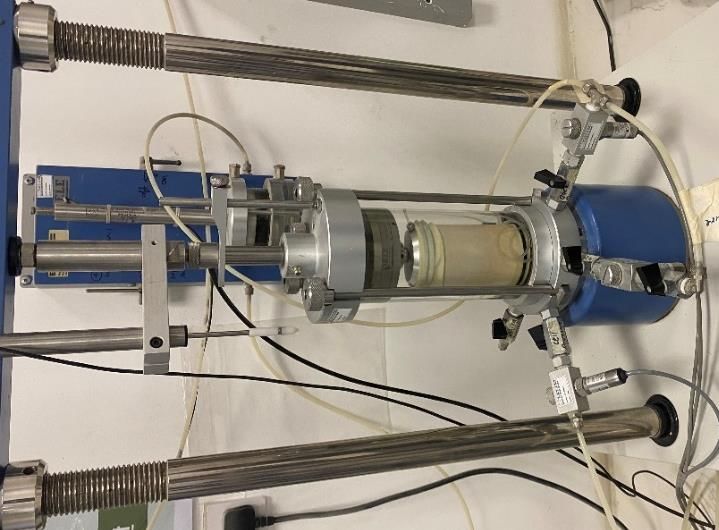
Table 4. Calculation results for MC parameters for SL (top), MSH (middle) and RUS (bottom) according to Hoek & Brown (1997)6.00 HB simulated
Mohr circle
5.00 MC tangent
Tangent point
4.00
Radial lline
3.00
τ
2.00
1.00
σni
0.00
0.00 1.00 2.00 3.00 4.00 5.00 6.00 7.00 8.00 9.00 10.00 11.00 12.00
σn
5.00
4.00
3.00
τ
2.00
1.00
σni
0.00
0.00 1.00 2.00 3.00 4.00 5.00 6.00 7.00 8.00 9.00
σn
4.00
3.00
τ 2.00
1.00
σni
0.00
0.00 1.00 2.00 3.00 4.00 5.00 6.00 7.00
σn
Figure 2. Graphics of MC conversion for SL (top), MSH (middle) and RUS (bottom) according to Hoek & Brown (1997)4 Verification
In comparing the above methods, for results on Qatari rocks (table 1), we first have to note the result ranges and variability which is
present with all methods, except for Hoek & Brown (1997) approach. As already mentioned earlier, the method of converting
directly from triaxial tests with low confinement loads gives exceedingly high friction angles, whereas the cohesion results are in
reasonable agreement with Hoek & Brown (1997) method. Cohesion values from Fourniadis (2010) and Karagkounis et al. (2016)
are considerably lower. From all this, we can only preliminarily conclude that Hoek & Brown (1997) method likely gives the most
realistic MC values. Reservations still remain however, being that in this case Hoek & Brown (1997) approach can only provide the
simulated triaxial values, based on the most educated estimates of mi from table 2. The author reiterates here that correctly performed
triaxial tests, with confinement load of up to 50 % of average UCS value are the most accurate method of determining HB
parameters, followed by conversion to MC parameters.
However, if we compare the results from this technical note with results of other selected authors who obtained MC values for
sedimentary rocks, we can observe the findings in the below table 4. We can see that friction angle values reach above 35 degrees,
predominantly only for substantial cohesion values. For cohesion values just above zero or on the lower side, the friction angles
rarely exceed 30 degrees, or only go slightly over. We can say that this confirms with greatest probability that Hoek & Brown (1997)
approach gives the most accurate cohesion and angle of friction values. This further puts values of Fourniadis (2010) within
acceptable range, whereas Karagkounis et al. (2016) value ranges are likely exceedingly high.
In their work Latapie and Lochaden (2016) have criticized the Hoek & Brown (2002) conversion method to MC parameters, citing
the fact that it only uses confinement stress range up to 0.25 UCS, as a shortcoming (in the same manner as Hoek & Brown 1997
procedure), in particular for slope and retaining wall problems. They also cited the fact that Intermediate Ground materials are
governed by shear strength of the rock mass, rather than by discontinuities, as is often the case for hard, more intact rocks, and
Karagkounis et al. (2016) have implicated that this applies to Qatari rock masses. What concerns this issue, it was already shown by
Vucemilovic et al. (2021) that Qatari rock masses, for most part, are not Intermediate Ground material, and even softest RUS
member characteristics conform to a very limited extent to its’ criteria (average UCS was recorded at 12.9 MPa and transitional HB
variables’ changes from Carvalho 2007 are minor as seen in table 2). Furthermore, if we consider the tendencies of most triaxial test
results, further moving along the HB envelope curve towards higher σ1 – σ3 pairs only yields a flatter tangent (smaller φ) and a slight
increase in cohesion. Thus, employing of a σ3 range higher than 0 < σ3 < 0.25 UCS would presumably not yield higher φ values.Table 5. Summary of MC parameters for sedimentary rocks from other selected authors
UCS magnitude/ φ magnitude/ range c magnitude/
Author Rock type
range [MPa] [deg] range [MPa]
Bejarbaneh et al (2015) Iranian shale 17.45 32.4 5.83
Armaghani et al. (2014) Iranian shale 19.0 – 47.0 20.5 – 40.1 -
Bell (2007) Kirkheaton mudrock 34.4 – 69.9 38 – 47 0 – 5.0
Shen et al. (2012) theoretical 30.0 20.96 – 26.71 0.15 – 0.21
Goodman (1989) Bartesville sandstone - 37.2 8.0
Goodman (1989) Indiana limestone - 42.0 6.7
Goodman (1989) Hasmark dolomite - 35.5 22.8
Goodman (1989) chalk - 31.5 0
Miščević & Vlastelica (2009) Croatian marl - 32.0 – 35.0 6.0 – 7.0
This technical note Qatari rocks 12.9 – 26.7 24.6 – 28.9 0.69 – 1.12
Fourniadis (2010) Qatari rocks (SL only) 5.0 – 12.0 21.0 – 32.0 0.14 – 0.65
Karagkounis et al. (2016) Qatari rocks 4.0 – 23.0 21.0 – 48.0 0.03 – 0.44
5 Conclusions
Calculation of Mohr-Coulomb parameters for Qatari rocks should follow either after correctly performing triaxial tests
(confinement load up to 0.5 UCS after Hoek 1980a), and after obtaining the resulting mi values; OR after correctly estimating
the mi values via other means, and simulating the triaxial results with mi, GSI and UCS results as per this technical note in
accordance with Hoek & Brown (1997), Appendix C procedure.
This paper has also demonstrated that mi values follow the tendency of the R-index which represents the ratio of compressive
to tensile intact strength, and that tensile strength of subject Qatari rocks drops more pronouncedly with depth than the drop of
compressive strength (as shown in Vucemilovic et al. 2021) which points to mi increasing with depth, at least down to RUS
Calcareous layer.
This method gives a range of friction angles for Doha intact rocks between 24.0 – 30.0 degrees whereas the cohesion values
are between 0.5 – 1.5 MPa. The values are reported down to deepest layer which is RUS calcareous.
Acknowledgements
The author wishes to thank Dr. Evert Hoek for providing kind assistance on his 1997 paper and method.Declarations Funding: This research was not founded by any party. Conflicts of interest: The author declares that he has no known competing financial interests or personal relationships that influenced the work reported in this paper. Availability of data and material: The datasets generated during and/or analyzed during the current study are not publicly available due to proprietary confidentiality but are available from the author on reasonable request. References Armaghani DJ, Hajihassani M, Bejarbaneh BY, Marto A, Mohamad ET (2014), Indirect measure of shale shear strength parameters by means of rock index tests through an optimized artificial neural network, Measurement, Volume 55, 2014, Pages 487-498, ISSN 0263- 2241, https://doi.org/10.1016/j.measurement.2014.06.001. Arshadnejad S, Nick N (2016) Empirical models to evaluate of “mi ” as an intact rock constant in the Hoek-Brown rock failure criterion. 19th Southeast Asian Geotechnical Conference & 2nd AGSSEA Conference (19SEAGC & 2AGSSEA) Kuala Lumpur 31 May – 3 June 2016 ASTM D7012-10 (2010), Standard Test Method for Compressive Strength and Elastic Moduli of Intact Rock Core Specimens under Varying States of Stress and Temperatures, ASTM International, West Conshohocken, PA, 2010, www.astm.org Bejarbaneh BY, Armaghani DJ, Amin MFM (2015), Strength characterisation of shale using Mohr–Coulomb and Hoek–Brown criteria, Measurement, Volume 63, 2015, Pages 269-281, ISSN 0263-2241, https://doi.org/10.1016/j.measurement.2014.12.029. Bell FG (2007), Engineering Geology (Second Edition), Butterworth-Heinemann, Elsevier Cai M (2009) Practical Estimates of Tensile Strength and Hoek–Brown Strength Parameter mi of Brittle Rocks. Rock Mechanics and Rock Engineering. 43. 167-184. 10.1007/s00603-009-0053-1. Carter TG, Diederichs MS, Carvalho, JL (2008) Application of modified Hoek–Brown transition relationships for assessing strength and post yield behavior at both ends of the rock competence scale. Proceedings 6th International Symposium on Ground Support in Mining and Civil Engineering Construction, SAIMM, Johannesburg, pp. 37–60. Carter, A. Dyskin, R. Jeffrey (eds), © 2008 Australian Centre for Geomechanics, Perth, ISBN 978-0-9804185-5-2 Carvalho JL, Carter TG, and Diederichs MS (2007) An approach for prediction of strength and post-yield behavior for rock masses of low intact strength. Rock Mechanics: Meeting Society’s Challenges and Demands, Proceedings 1st Canada – U.S. Rock Mechanics Symposium, Taylor and Francis, Leiden, 1, pp. 249–257. Fourniadis I (2010) Geotechnical Characterization of the Simsima Limestone (Doha, Qatar), GeoShanghai International Conference 2010 June 3-5, 2010 | Shanghai, China, https://doi.org/10.1061/41105(378)38 Goodman RE (1989). Introduction to Rock Mechanics. Wiley, New York, NY. Hoek, E (1983). Strength of jointed rock masses, 23rd. Rankine Lecture. Géotechnique 33(3), 187-223.
Hoek E (1990). Estimating Mohr-Coulomb friction and cohesion values from the Hoek-Brown failure criterion. Intnl. J. Rock Mech. &
Mining Sci. & Geomechanics Abstracts. 12(3), 227-229.

Hoek E, Brown ET (1980a) Underground excavations in rock. London: Institute of Mining and Metallurgy

Hoek E, Brown ET (1997) Practical estimates of rock mass strength. Int J Rock Mech Min Sci 34:1165–1186

Hoek E, Carranza-Torres C, Corkum B (2002) Hoek-Brown failure criterion – 2002 Edition. Conference: Proc. NARMS-TAC
Conference, Toronto, 2002, 1, 267-273

Hoek E, Kaiser PK, Bawden WF (1995) Support of underground excavations in hard rock. Rotterdam: A.A. Balkema.

Hoek E, Wood D and Shah S (1992). A modified Hoek-Brown criterion for jointed rock masses. Proc. rock characterization, symp. Int.
Soc. Rock Mech.: Eurock ‘92, (J.Hudson ed.). 209-213.

Karagkounis N, Latapie B, Sayers K, Mulinti SR (2016) Geology and geotechnical evaluation of Doha rock formations. Geotechnical
Research, 2016, 3(3), 119–136, http://dx.doi.org/10.1680/jgere.16.00010

Latapie B, Lochaden ALE (2015) Range of confining pressures for the Hoek–Brown criterion. Geotechnical Research, 2015, 2(4), 148–
154, http://dx.doi.org/10.1680/jgere.15.00008

Miščević P & Vlastelica G. (2009). Shear strength of weathered soft rock - proposal of test method additions. Proc. Reg. Sym. on Rock
Eng. in Diff. Gr. Cond. - Eurock 2009. 303-308.

Shen J, Priest SD, Karakus M (2012), Determination of Mohr–Coulomb Shear Strength Parameters from Generalized Hoek–Brown
Criterion for Slope Stability Analysis, Rock Mech Rock Eng (2012) 45:123–129, DOI 10.1007/s00603-011-0184-z

Vučemilović H, Mulabdić M, & Miščević P (2021), Corrected Rock Fracture Parameters and Other Empirical Considerations for the
Rock Mechanics of Rock Masses of Doha, Qatar. Geotech Geol Eng 39, 2823–2847 (2021). https://doi.org/10.1007/s10706-020-01658-
y
You can also read