ONLINE PARAMETER INFERENCE FOR THE SIMULA- TION OF A BUNSEN FLAME USING HETEROSCEDASTIC BAYESIAN NEURAL NETWORK ENSEMBLES
←
→
Page content transcription
If your browser does not render page correctly, please read the page content below
Published as a workshop paper at ICLR 2021 SimDL Workshop

                                         O NLINE PARAMETER INFERENCE FOR THE SIMULA -
                                         TION OF A B UNSEN FLAME USING HETEROSCEDASTIC
                                         BAYESIAN NEURAL NETWORK ENSEMBLES
                                          Maximilian L. Croci, Ushnish Sengupta & Matthew P. Juniper
                                          Department of Engineering
                                          University of Cambridge
                                          Cambridge, United Kingdom
                                          mlc70@cam.ac.uk
arXiv:2104.13201v1 [cs.LG] 26 Apr 2021

                                                                                       A BSTRACT

                                                     This paper proposes a Bayesian data-driven machine learning method for the on-
                                                     line inference of the parameters of a G-equation model of a ducted, premixed
                                                     flame. Heteroscedastic Bayesian neural network ensembles are trained on a li-
                                                     brary of 1.7 million flame fronts simulated in LSGEN2D, a G-equation solver,
                                                     to learn the Bayesian posterior distribution of the model parameters given obser-
                                                     vations. The ensembles are then used to infer the parameters of Bunsen flame
                                                     experiments so that the dynamics of these can be simulated in LSGEN2D. This
                                                     allows the surface area variation of the flame edge, a proxy for the heat release
                                                     rate, to be calculated. The proposed method provides cheap and online parameter
                                                     and uncertainty estimates matching results obtained with the ensemble Kalman
                                                     filter, at less computational cost. This enables fast and reliable simulation of the
                                                     combustion process.1

                                         1       I NTRODUCTION

                                         Simulation-based digital twins of physical systems are becoming cheaper to use due to improve-
                                         ments in computer processing power and storage (Fuller et al., 2020). Data-driven machine learning
                                         methods for the inference of digital twin model parameters from experiments are made possible in
                                         part due to the possibility of creating cheap synthetic data sets at scale. These methods can also
                                         address the need to do bring down the computational cost of parameter inference such that these
                                         models may be updated in real-time (online) using the latest sensor observations.
                                         In the design of modern rocket engines and gas turbines, simulation of the combustion process (the
                                         flame) can be used to design out thermoacoustic instabilities which would otherwise lead to catas-
                                         trophic damage (Juniper & Sujith, 2018). Thermoacoustic instabilities are driven by the coupling of
                                         the heat release rate of the flame and the acoustics in the combustor (Strutt, 1878). It is therefore
                                         necessary to model the flame dynamics such that the heat release rate is quantitatively accurate.
                                         The G-equation (Williams, 1985) is the kinematic model used in LSGEN2D (Hemchandra, 2009)
                                         to simulate a ducted, premixed flame such as that from a Bunsen burner. By tuning the parameters
                                         of the G-equation model to fit a Bunsen flame experiment, a digital twin of the flame is created and
                                         its surface area variation in time, which is a proxy for the heat release rate, can be calculated. The
                                         ensemble Kalman filter (EnKF) is the current state-of-the-art, which iteratively performs Bayesian
                                         inference of the G-equation parameters from G-equation model forecasts generated in LSGEN2D
                                         and observations of the flame edge (Yu et al., 2019). The model forecasting is expensive, however,
                                         which makes the EnKF too expensive to be used online. We propose to infer online the G-equation
                                         parameters of Bunsen flame experiments using a heteroscedastic Bayesian neural network ensem-
                                         ble (Sengupta et al., 2020a;b). In an expensive offline step, the ensemble learns a surrogate for the
                                         Bayesian posterior distribution of the parameters given observations of the flame front from a library
                                         of pairs of G-equation parameters and corresponding flame front shapes generated in LSGEN2D.
                                             1
                                                 Code available at: https://github.com/nailimixaM/iclr-2021-baynne

                                                                                              1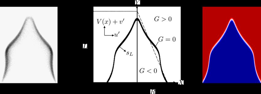
Published as a workshop paper at ICLR 2021 SimDL Workshop

The ensemble can then be used to infer online the parameters of the model for simulation of the
Bunsen flames.

2     B UNSEN FLAME EXPERIMENT AND SIMULATIONS
2.1   B UNSEN FLAME EXPERIMENT

A Bunsen burner is placed inside a transparent duct and a high-speed camera is used to take images
of the Bunsen flame at a frame rate of fs = 2500 frames per second and a resolution of 1200 × 800
pixels. Speakers force the flame at frequencies in the range 250 Hz to 450 Hz. The gas composition
(methane, ethene and air) and flow rate are varied using mass flow controllers. By varying the
forcing frequency and amplitude and gas composition and flow rate, flames with different aspect
ratios, propagation speeds and degrees of cusping of the flame front are observed. In some cases,
the flame front cusping leads to pinch-off at the flame tip. For each of the 270 different flame
operating conditions, 500 images are taken.
The flame images are processed to find a single-valued discretisation of the flame front, x = f (y).
First, the pixel intensities are thresholded and a position x for every vertical position y is found by
weighted interpolation of the thresholded pixels, where the weights are the pixel intensities. Next,
splines with 28 knots are used to smooth the (x, y) coordinates. Each flame image is therefore
converted into a 90 × 1 vector of flame front x coordinates x (as the y coordinates are the same
for all flames, they are discarded). Observation vectors z are created by stacking 10 subsequent x
vectors. These observation vectors are used for inference with the neural networks. All 500 images
of each Bunsen flame are processed in this way.

2.2   F LAME FRONT MODEL

In this paper we use a kinematic model of the flame front as a boundary between reactants and
products (see Figure 1). The flame front is defined to be the G = 0 contour of a scalar field
G(x, y, t). Regions of negative and positive G correspond to unburnt and burnt gases respectively
(the magnitude of G does not have a useful meaning). The position of the flame front in space and
time is governed by:
                                       ∂G
                                             + v · ∇G = sL |∇G|,                                      (1)
                                        ∂t
where v is a prescribed velocity field and sL is the laminar flame speed: the speed at which the
flame front propagates normal to itself into the reactants. The flame speed sL = s0L (1 − Lκ) is
a function of the unstretched (adiabatic) flame speed s0L , the flame curvature κ and the Markstein
length L, and is insensitive to pressure variations. The unstretched flame speed s0L depends only on
the flame chemistry. The velocity field v = u0 i + (V (x) + v 0 ) j comprises a parabolic base flow
                                   x 2
profile V (x) = V (1 + α(1 − 2( R    ) )) and superimposed continuity-obeying velocity perturbations
u (x, y, t) = V  sin(St( R y − t)) and v 0 (x, y, t) = − V KSt
  0                       K                                              K
                                                             R x cos(St( R y − t)) where α determines
the shape of the base flow profile (α = 0 is uniform flow, α = 1 is Poiseuille flow),  is the amplitude
of the vertical velocity perturbation with phase speed V /K, St = 2πf Rβ/V is the Strouhal number
with forcing frequency f and flame radius R, and β is the aspect ratio of the unperturbed flame. The
parameters K, , L, α, St and β are tuned to fit an observed flame shape.

2.3   S IMULATED FLAME FRONT LIBRARY

A library of simulated flame fronts with known parameters K, , L, α, St and β is created for neural
network training. The parameter values are sampled using quasi-Monte Carlo sampling to ensure
good coverage of the parameter space. The parameters are sampled from the following ranges:
0.0 < K ≤ 1.5, 0.0 <  ≤ 1.0, 0.02 ≤ L ≤ 0.08, 0.0 ≤ α ≤ 1.0, 2.0 ≤ β ≤ 10.0 and
0.08 ≤ f /fs ≤ 0.20. The values of St are calculated by additionally sampling 0.002 ≤ R ≤ 0.004
m and 1 ≤ V ≤ 5 m/s and calculating St = 2πf Rβ/V . The parameters are sampled 8500 times,
normalised to between 0 and 1 and recorded in target vectors {t = [K, , L, α, St, β]}.
For each of the 8500 unique parameter configurations, LSGEN2D iterates the G-equation model of
the flame front until it converges to the corresponding forced cycle. For each of the 200 forced cycle
G field states produced by LSGEN2D, the flame front is found by interpolating the G values. This

                                                   2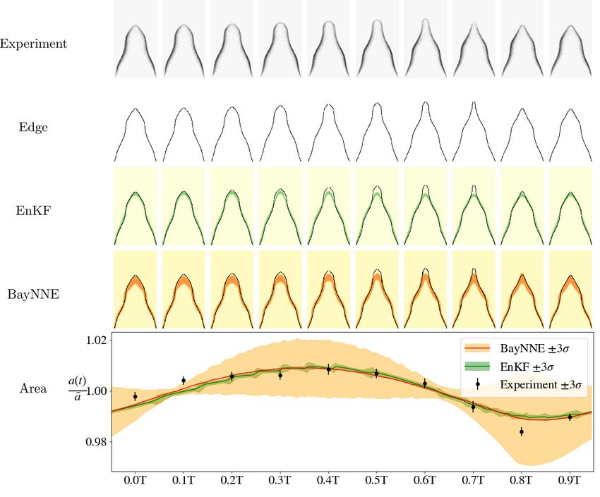
Published as a workshop paper at ICLR 2021 SimDL Workshop

Figure 1: (Left) Image of a Bunsen flame. (Middle) G-equation model of the flame front. (Right)
Simulated flame in LSGEN2D.

results in a x = f (y) discretisation and the vectors x of x coordinates are recorded. Observation
vectors z are created by stacking 10 subsequent x vectors. There are 200 observation vectors created
from every cycle, resulting in a library of 1.7 × 10⁶ observation-target parameter pairs {(z, t)}. This
library is split 80%-20% into training and testing data sets.

3    I NFERENCE USING HETEROSCEDASTIC                      BAYESIAN NEURAL NETWORK
     ENSEMBLES

We assume the posterior probability distribution of the parameters given the observations can be
modelled by a neural network: pθ (t|z) with its own parameters θ. We assume this posterior distri-
bution has the form:
                                     pθ (t|z) = N (t; µ(z), Σ(z)) ,                                (2)
                         2
where Σ(z) = diag(σ (z)). This encodes our assumption that the parameters are all mutually
independent given the observations z. The architecture of a single neural network is shown in Figure
2. Each neural network comprises an input layer, four hidden layers with ReLU activations and
two output layers: one for the mean vector µ(z) and one for the variance vector σ 2 (z). The output
layer for the mean uses a sigmoid activation to restrict outputs to the range (0, 1). The output layer
for the variance uses an exponential activation to ensure positivity. An ensemble of M = 20 such
neural networks is initialised, each with unique initial weights θj,anc sampled from a Gaussian prior
distributions according to He initialisation (He et al., 2015).
For a single observation z, the j-th neural network in the ensemble produces a sample of the posterior
with an associated estimate of the aleatoric noise in the observations: µj (z), σj2 (z). This is achieved
by using the loss function Lj :
                   T         −1                                                   T
Lj = (µj (z) − t) Σj (z)        (µj (z) − t) + log (|Σj (z) |) + (θj − θanc,j ) Σ−1
                                                                                 prior (θj − θanc,j ) .
                                                                                                  (3)
The loss function comprises the negative log of the Gaussian likelihood function (probability of the
observations given the targets, first two terms) and a regularising (penalty) term. By regularising
about parameter values drawn from a prior distribution, the NNs produce samples from the posterior
distribution. This is called randomised maximum a-posteriori (MAP) sampling (Pearce et al., 2020).
Once converged, the prediction from the ensemble for an observation z is therefore a mixture of M
Gaussians each centered at their respective means µj (z). This mixture is approximated by a single
                                                                                                     Σ µ (z)
multivariate Gaussian posterior distribution p(t|z) ≈ N (t; µ(z), Σ(z)) with mean µ(z) = j Mj
                                                                2           2                  2
                                                            Σj σj (z)  Σj µ (z)       Σj µj (z)
and covariance Σ(z) = diag(σ 2 (z)) where σ 2 (z) =            M      + Mj −              M        following
similar treatment in Lakshminarayanan et al. (2017). This is done for every observation vector z.
                                                                       2
The posterior distribution p(t|zi ) with the smallest total variance σi,tot = ||σ 2 (zi )||1 is chosen as the
best guess to the true posterior. The M parameter samples from the chosen posterior are used for
re-simulation, which allows us to check the predicted flame shapes and to calculate the normalised
area variation over one cycle.

                                                     3
Published as a workshop paper at ICLR 2021 SimDL Workshop
Figure 2: Architecture of a single neural network. The input and hidden layers have 900 nodes each,
while the output layers have 6 nodes each. All layers are fully connected (FC). Rectified Linear
Unit (ReLU) activation functions are used for the hidden layers and sigmoid and exponential (Exp)
activation functions are used for the mean and variance ouput layers respectively.
4 R ESULTS
The ensemble is trained for 5000 epochs and evaluated on the Bunsen flame image data. Parameter
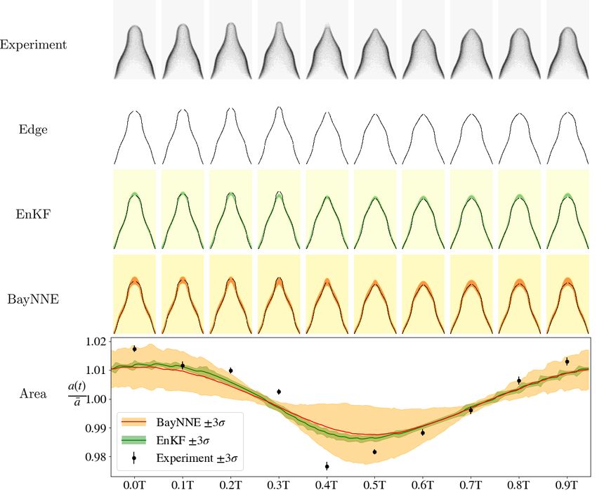
predictions for an observation vector z take O(10−4 ) seconds on an Nvidia P100 GPU. Figure 3
show the results of inference and simulation of two different Bunsen flames. The BayNNE predicts
flame shapes in good agreement with the experiments: the root mean square distances between
the simulated and Bunsen flame shapes of 5 different Bunsen flames ranges from 0.017 units to
0.024 units, with mean 0.019 units (where the flame radius is 1 unit). These results show that the
BayNNE’s parameter estimates match those of the EnKF and require O(108 ) less computing power.
The uncertainty in the BayNNE’s predictions is greater than that of the EnKF due to the calcu-
lated posterior being the probability of the parameters given 10 flame images, whereas the EnKF
considers all 500 flame images of the Bunsen flame. Unfortunately, it is not possible to combine
the BayNNE’s parameter estimates without knowledge of the probability distribution between the
observation vectors. Any two observation vectors are not independent as knowledge about the first
restricts our expectation of the second to a likely set of forced cycle states. Future work will address
this limitation by using alternative neural network architectures, such as long-short term memory
networks (Hochreiter & Schmidhuber, 1997), that are better suited to time-series data.
5 C ONCLUSIONS
This work proposes a method for inferring the parameters of the G-equation model of a Bun-
sen flame for simulation purposes. Bayesian inference of the parameters and their uncertainties
is performed using heteroscedastic Bayesian neural network ensembles. The neural networks are
trained on a library of synthetic flame front observations created using LSGEN2D. Once trained, the
Bayesian neural network ensemble accurately predicts the parameters and uncertainties from just
10 images of the Bunsen flame. The simulated flames with parameters predicted by the ensemble
agree with the experiments, and the surface area variation, which is a proxy for the heat release rate,
is calculated. A quantitatively accurate digital twin of the Bunsen flame is therefore created. Fu-
ture work will focus on improving the parameter and uncertainty estimates by leveraging alternative
neural network architectures.
D ISCLOSURE OF F UNDING
This project has received funding from the UK Engineering and Physical Sciences Research Council
(EPSRC) award EP/N509620/1 and from the European Union’s Horizon 2020 research and innova-
tion program under the Marie Skłodowska-Curie grant agreement number 766264.
4Published as a workshop paper at ICLR 2021 SimDL Workshop
Figure 3: Results of inference using the BayNNE method compared to the EnKF method for the
simulation of two different Bunsen flames. The flame images are preprocessed to find the flame
front and then used for inference. The green and orange bands in the EnKF and BayNNE predicted
flame shape plots are regions of high likelihood. The normalised area variations over one period of
the simulated flames show good agreement with the experiments.
5Published as a workshop paper at ICLR 2021 SimDL Workshop
R EFERENCES
A. Fuller, Z. Fan, C. Day, and C. Barlow. Digital twin: Enabling technologies, challenges and open
research. IEEE Access 8:108952–108971, 2020.
K. He, X. Zhang, S. Ren, and J. Sun. Delving deep into rectifiers: Surpassing human-level perfor-
mance on imagenet classification. IEEE International Conference on Computer Vision (ICCV),
pp. 1026–1034, 2015.
S. Hemchandra. Dynamics of Turbulent Premixed Flames in Acoustic Fields. PhD Thesis, 2009.
S. Hochreiter and J Schmidhuber. Long short-term memory. Neural Computation, 9(8):1735–1780,
1997.
M. P. Juniper and R. Sujith. Sensitivity and nonlinearity of thermoacoustic oscillations. Annual
Review of Fluid Mechanics, 2018.
B. Lakshminarayanan, A Pritzel, and C. Blundell. Simple and scalable predictive uncertainty estima-
tion using deep ensembles. 31st Conference on Neural Information Processing Systems (NIPS),
Long Beach, CA, USA, 2017.
T. Pearce, M. Zaki, A. Brintrup, N. Anastassacos, and A. Neely. Uncertainty in neural networks:
Bayesian ensembling. International Conference on Artificial Intelligence and Statistics, 2020.
U. Sengupta, M. Amos, J. Scott Hosking, C. E. Rasmussen, M. P. Juniper, and P. J. Young. Ensem-
bling geophysical models with bayesian neural networks. 34th Conference on Neural Information
Processing Systems (NeurIPS), Vancouver, Canada, 2020a.
U. Sengupta, M. L. Croci, and M. P. Juniper. Real-time parameter inference in reduced-order flame
models with heteroscedastic bayesian neural network ensembles. Machine Learning and the
Physical Sciences Workshop at the 34th Conference on Neural Information Processing Systems
(NeurIPS), Vancouver, Canada, 2020b.
J. W. Strutt. The Theory of Sound (Vol II). Macmillan and Co., 1878.
F. A. Williams. Turbulent combustion. The mathematics of combustion, pp. 97–131, 1985.
H. Yu, M. P. Juniper, and L. Magri. Combined state and parameter estimation in level-set methods.
J. Comp. Phys., 399, 2019.
A S UPPLEMENTARY MATERIAL : H YPERPARAMETER SETTINGS
Table 1: Hyperparameter settings.
Hyperparameter Value
Training
Train-test split 80:20
Batch size 2048
Epochs 5000
Optimiser Adam
Learning rate 10−3
Architecture
Input units 900
Hidden layers 4
Units per hidden layer 900
Output layers 2
Units per output layer 6
Ensemble size 20
6You can also read